$\ell_1$-minimization method for link flow correction
Penghang Yin, Zhe Sun, Wenlong Jin, Jack Xin

TL;DR
This paper introduces an $ ext{l}_1$-minimization approach for correcting inconsistent link flow data in road networks, effectively identifying and fixing corrupted sensors under certain recoverability conditions, even with measurement noise.
Contribution
It develops a novel $ ext{l}_1$-minimization method with a recoverability condition to accurately correct corrupted traffic flow data, including an analytical framework and algorithm for robustness.
Findings
Method accurately corrects corrupted link flows in synthetic and real data.
Recoverability condition ensures robustness to sensor miscounts.
Provides bounds on correction errors under measurement noise.
Abstract
A computational method, based on -minimization, is proposed for the problem of link flow correction, when the available traffic flow data on many links in a road network are inconsistent with respect to the flow conservation law. Without extra information, the problem is generally ill-posed when a large portion of the link sensors are unhealthy. It is possible, however, to correct the corrupted link flows \textit{accurately} with the proposed method under a recoverability condition if there are only a few bad sensors which are located at certain links. We analytically identify the links that are robust to miscounts and relate them to the geometric structure of the traffic network by introducing the recoverability concept and an algorithm for computing it. The recoverability condition for corrupted links is simply the associated recoverability being greater than 1. In a more…
Click any figure to enlarge with its caption.
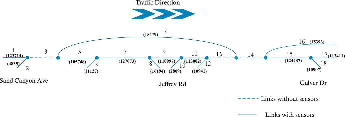 Figure 1
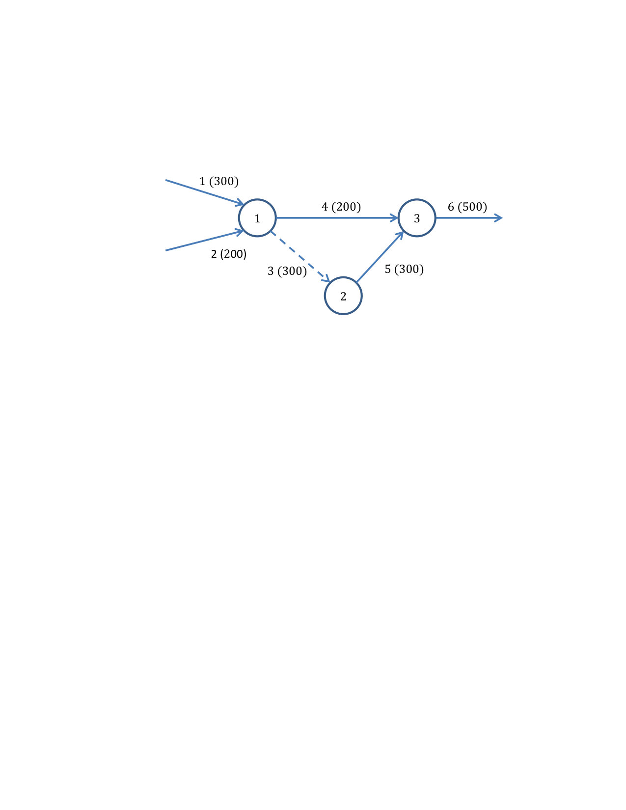 Figure 2
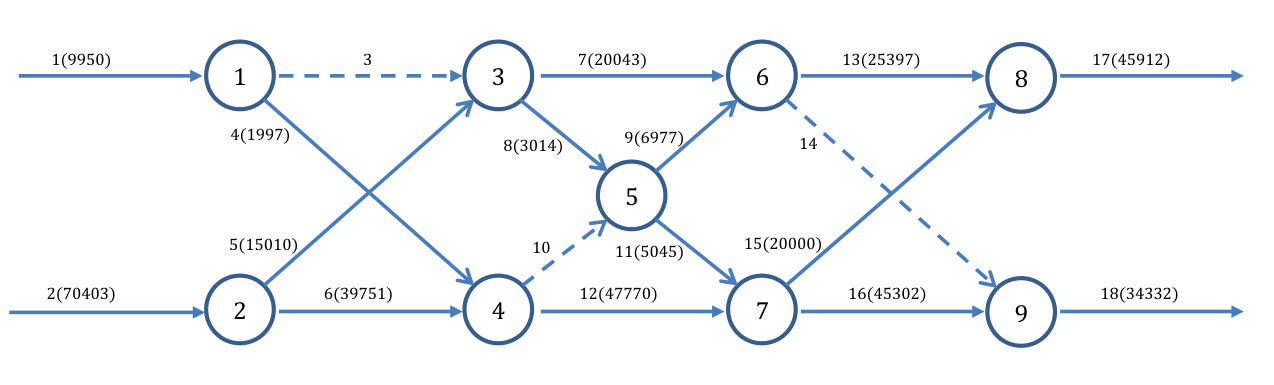 Figure 3
| Link ID | Ground-truth | Observation | Estimation | Estimation Error |
|---|---|---|---|---|
| 1 | 10000 | 9950 | 9950 | -10 |
| 2 | 70000 | 69887 | 69887 | -113 |
| 3 | 8000 | N/A | 7953 | -47 |
| 4 | 2000 | 1997 | 1997 | -3 |
| 5 | 15000 | 15010 | 15104 | 104 |
| 6* | 55000 | 39751 | 54783 | -217 |
| 7 | 20000 | 20043 | 20043 | 43 |
| 8 | 3000 | 3014 | 3014 | 14 |
| 9 | 7000 | 6977 | 6977 | 23 |
| 10 | 9000 | N/A | 9009 | 9 |
| 11 | 5000 | 5045 | 5046 | 46 |
| 12 | 48000 | 47770 | 47771 | -229 |
| 13 | 25500 | 25397 | 25505 | 5 |
| 14 | 1500 | N/A | 1515 | 15 |
| 15 | 20000 | 20000 | 20000 | 0 |
| 16* | 33000 | 45302 | 32817 | -183 |
| 17 | 45500 | 45912 | 45505 | 5 |
| 18 | 34500 | 34332 | 34332 | -168 |
| Link ID | Observation | Estimation | Difference | Percentage Difference |
|---|---|---|---|---|
| 1 | 123714 | 123714 | 0 | 0.0% |
| 2 | 4835 | 4835 | 0 | 0.0% |
| 3 | N/A | 128549 | N/A | N/A |
| 4 | 15479 | 15479 | 0 | 0.0% |
| 5 | 105748 | 113070 | 7322 | 6.9% |
| 6 | 11127 | 13661 | 2534 | 22.8% |
| 7 | 127073 | 126731 | -342 | -0.3% |
| 8 | 16194 | 16194 | 0 | 0.0% |
| 9 | 110997 | 110537 | -460 | -0.4% |
| 10 | 2809 | 2757 | -52 | -1.9% |
| 11 | 113002 | 113295 | 293 | 0.3% |
| 12 | 10941 | 10941 | 0 | 0.0% |
| 13 | N/A | 124236 | N/A | N/A |
| 14 | N/A | 139715 | N/A | N/A |
| 15 | 124437 | 124322 | -115 | -0.1% |
| 16 | 15393 | 15393 | 0 | 0.0% |
| 17 | 113411 | 113413 | 2 | 0.0% |
| 18 | 10907 | 10909 | 2 | 0.0% |
Peer Reviews
No public reviews on file for this paper yet. If you reviewed it on a platform where reviews are public (OpenReview, ICLR, NeurIPS, ICML), you can paste yours below so the community can read it here.
Videos
No videos yet. Explain this paper in a talk, walkthrough, or lecture? Add one.
Taxonomy
TopicsProbabilistic and Robust Engineering Design · Traffic control and management · Power System Optimization and Stability
-minimization method for link flow correction
Penghang Yin , Zhe Sun, Wen-Long Jin, and Jack Xin Department of Mathematics, University of California, Los Angeles, Los Angeles, CA, 90095. Email: [email protected] of Civil and Environmental Engineering, Institute of Transportation Studies, 4040 Anteater Instruction and Research Bldg, University of California, Irvine, CA 92697-3600. Email: [email protected] of Civil and Environmental Engineering, California Institute for Telecommunications and Information Technology, Institute of Transportation Studies, 4038 Anteater Instruction and Research Bldg, University of California, Irvine, CA 92697-3600. Email: [email protected]. Corresponding author.Department of Mathematics, University of California, Irvine, Irvine, CA 92697. Email: [email protected].
Abstract
A computational method, based on -minimization, is proposed for the problem of link flow correction, when the available traffic flow data on many links in a road network are inconsistent with respect to the flow conservation law. Without extra information, the problem is generally ill-posed when a large portion of the link sensors are unhealthy. It is possible, however, to correct the corrupted link flows accurately with the proposed method under a recoverability condition if there are only a few bad sensors which are located at certain links. We analytically identify the links that are robust to miscounts and relate them to the geometric structure of the traffic network by introducing the recoverability concept and an algorithm for computing it. The recoverability condition for corrupted links is simply the associated recoverability being greater than 1. In a more realistic setting, besides the unhealthy link sensors, small measurement noises may be present at the other sensors. Under the same recoverability condition, our method guarantees to give an estimated traffic flow fairly close to the ground-truth data and leads to a bound for the correction error. Both synthetic and real-world examples are provided to demonstrate the effectiveness of the proposed method.
Keywords: Link flow correction; -minimization; flow conservation law; recoverability; exact recovery; correction bound.
1 Introduction
Link volume/flow data is an important data source in both long-term planning and short-term operation applications. The examples include but are not limited to signal timing, toll road pricing, origin-destination trip matrix estimation, transportation planning, traffic safety (e.g. [14, 16, 19, 17] and the references therein).
The flow conservation in a traffic network implies that the total in-flow equals the total out-flow at each non-centroid node. The centroids are nodes where traffic originates/is destined to, and non-centroids nodes denotes all the other nodes. Practically, when looking at traffic flow counts over a sufficiently long time period (e.g. daily cumulative flow), we expect that the sum of cumulative link flows entering the non-centroid node equals the sum of cumulative link flows leaving it.
The flow conservation law is an important property, which has been exploited in many different applications. For example, the widely used first-order traffic flow model, the LWR model [15, 22], is derived based on the conservation of traffic. In [6], the authors mentioned that a path flow estimator (PFE) needs reasonably consistent link flows, meaning that the flow conservation law should be satisfied within a certain error bound, to reproduce feasible path flow solutions.
In practice, the flow conservation law can be violated due to numerous flow measuring errors; i.e., the observed flow counts are generally corrupted and cause data inconsistency issues. In [23], the network sensor health problem (NSHP) ([23]) is proposed to evaluate individual sensors’ health indices based on the level of flow data consistency. Assuming flow counting sensors are already installed on some of the links where at least one base set exists, the NSHP tries to find the least inconsistent base set that “minimizes the sum of squares of the differences between observed and calculated link flows”. The health index of a specific sensor is evaluated based on the frequency that it appears in the least inconsistent set.
Several studies have looked into the problem of correcting inconsistent flow data according to flow conservation. To solve a similar problem in transit planning, Kikuchi et al. [12] studied the passenger flow balancing problem and proposed a least square correction method to adjust the flows, so that the counts are conserved and close to the observed values. van Zuylen and Branston [25] assumed that the observed link flows follow probability distributions constrained by flow conservation. The study derived the formula for constrained maximum likelihood estimates of the link flows. Kikuchi et al. [13] examined and compared six different methods to adjust observed flow rate according to flow conservation. All of the methods have the same constraints but different objective functions. Vanajakshi and Rilett [24] studied flow inconsistency problem between neighboring upstream and downstream loop detectors. A nonlinear optimization problem is proposed to correct loop detector data, in the case when observed data violates flow conservation.
In summary, given the observed cumulative flows on different links, all of the existing flow correction methods adopted optimization approaches that try to meet the following principles:
- •
Ensure that flow conservation be followed exactly at all non-centroid nodes after adjustment using a set of constraints,
- •
Preserve the integrity of the observed data as much as possible by minimizing the distance between adjusted and observed flows.
However, all of the studies are limited to simple hypothetical networks or networks with simple topologies. Also, no systematic study has been done regarding the effectiveness and applicability of the methods.
In this study, we propose a method to estimate the true link flow from corrupted data on observed links as well as unobserved links via -minimization. Similar to the existing methods, the link flow correction method is also formulated as an optimization problem to minimize the difference between observed and estimated link flows. As an improvement over the existing methods, the node-based formulation of flow conservation is introduced to handle general road network where link flows are only observed on monitored links, not on all links as assumed in many existing studies. More importantly, we adopt the -minimization method from compressed sensing [4, 3] to analytically derive the condition for exact/stable recovery of the true cumulative flow counts.The norm is the unique convex sparsity promoting penalty. Though it is not differentiable, various efficient scalable numerical methods exist to date for its minimization [1, 2, 7, 9, 28] besides linear programming. In addition to norm, other non-convex sparsity promoting penalty functions can also be considered; see [29, 30, 18] and references therein. Their minimization is computationally more expensive than , and we shall leave such a study for a future work.
The rest of the paper is organized as follows. In section 2, we state the link flow correction problem formulation, the exact and stable recovery theorem, the recoverability condition and the connection with compressed sensing. In section 3, we use a toy example to illustrate the conditions for exact and stable link flow recovery. In section 4, we use real-world loop detector data as an application for this method. In both the toy and real world examples, the recoverability condition is verified analytically. The concluding remarks are in section 5.
Notations
Let us fix some notations. represents the real coordinate space of dimensions. Let , takes the norm of , and denotes the Euclidean () norm. Given any index set , counts the number of elements in ; is the complement set of . consists of the elements in restricted to the index set . denotes the vector containing zeros only, while denotes the identity matrix of order . For any matrix , is the transpose of ; is the submatrix of restricted to the row index set , and is the submatrix of restricted to the column index set ; e.g., extracts the first two rows of , and extracts the first two columns of . represents the kernel space of , while represents the range space of .
2 Methodology
2.1 Problem setup
Given a traffic network with non-centroid nodes only, the node-link incidence matrix with being the number of nodes and the number of links, can be expressed as
[TABLE]
Then is always of full (row) rank as proved in [21], and traffic flow data obeys the flow conservation:
[TABLE]
Suppose is the set of links whose link flows are observed, and . We call as “monitored set” thereafter. We assume that
[TABLE]
is the observed inconsistent flow data corrupted by sensing errors .
The flow correction problem is to derive an estimate of , denoted by , from the corrupted data . Here we impose an underlying assumption on for the flow correction problem to be well-posed. We will need the concept of base set introduced in [23].
Assumption 2.1**.**
* contains at least one base set , meaning that and is invertible.*
For the consistent data (i.e., ), of course we have since . Then the can be uniquely recovered by performing [21, 23]:
[TABLE]
If contains more than one base set, the recovered in the above from different will be consistent.
Assumption 2.1 is the sufficient and necessary condition for the whole link flows to be observable. It guarantees that the whole flow data can be deduced from at least one subset of the observed link flows. Without this assumption, however, some of the link flows cannot be estimated from available data and the problem is unsolvable [21], whether the measured flows are consistent or not.
2.2 Flow correction via -minimization
Since is of full row rank, is an -dimensional subspace of . Suppose is the matrix whose columns form a basis of . Since , we have
[TABLE]
As a result, must be of the form for some .
Remark 2.1**.**
Clearly the existence of is non-unique, but is invariant to the choice of and only depends on the structure of the traffic network. Indeed is the one in whose restriction on has the least absolute deviation from . So only depends on which is same as . Note that is the node-link matrix uniquely determined by the network structure.
The following result not only gives a concrete construction of , but also interprets in (2.2) as an estimate of for some base set (not necessarily a subset of ).
Theorem 2.1**.**
Let be any base set. Without loss of generality, suppose is partitioned as with being invertible. Then
[TABLE]
is a basis matrix of . Moreover, by choosing such , from (2.2) is an estimate of .
We will show the proof in Appendix C. Our proposed method consists of the following two steps:
We first solve an -minimization problem:
[TABLE]
That is, we seek an estimate of in the affine space with the least norm. The problem (2.2) can be efficiently solved by the alternating direction method of multipliers (ADMM) [2]; see Appendix A for the implementation details.
- 2.
is then estimated by
[TABLE]
may have non-integer entries, in this case, we can just perform rounding.
2.3 Connections with compressed sensing
Compressed sensing [3, 8] aims to recover a sparse signal (vector) from an under-determined linear system that generally has infinitely many solutions. It enables recovery of the signal from far fewer samples than required by the Nyquist-Shannon sampling theorem. Major ingredients of the standard compressed sensing technique include
- •
Sparsity: most of the entries in are zeros.
- •
-minimization: minimizing to exploit the sparsity of .
Let us return to the flow correction problem, which is in essence equivalent to the estimation of . In an extreme case, suppose all the sensors are bad, leading to large sensing errors. Without further information, it is clearly impossible to get a good estimate of from by any means. Intuitively, however, reconstructing is promising if most of the sensors record consistent flow data. Mathematically speaking, is sparse. The flow correction problem thus can be viewed as sparse error correction problem [4, 27], which is similar to compressed sensing. Note that, however, the flow correction problem deviates from the traditional compressed sensing problem, where the matrix would be random.
3 Correction results
Note that our proposed method does not take advantage of any prior information about the possible bad sensors. Apparently one can not always hope for a good estimation to , even if there is only one bad sensor in the network. For instance, in the network shown in Figure 1, if the sensor on link 1 gives very wrong count, then basically there is no way to reasonably correct this error because links 1 and 2 are equivalent in the topology of the network. With that said, without extra information, obtaining a good estimate of is possible only when the bad sensors are located at some particular links. These locations tolerating miscount are somehow determined by the network structure. In the following, we shall introduce the concept of recoverability.
Definition 3.1**.**
Given a network with node-link incidence matrix and monitored link set , we define the recoverability for the subset by
[TABLE]
which is a function of the subset and also determined by both the network structure and the monitored link set .
Since for some , then we can rewrite (3.4) as
[TABLE]
which resembles the classical Rayleigh quotient for the principal eigenvalue of the generalized eigenvalue problem [26]: if norm replaces the norm. The optimization of the ratio of two homogeneous functions of degree one has been studied [10] where an inverse power iterative algorithm was proposed. Based on [10], we propose an efficient algorithm to solve problem (3.5) which will be detailed in Appendix B.
3.1 Exact recovery
We first consider the case where some sensors are bad, which introduce inconsistency of the flow data. The following Theorem 3.1 asserts that when the bad sensors are located at certain link set whose size is expected to be small, then no matter how large the errors are, we are able to exactly recover from .
Theorem 3.1** (Exact recovery).**
Let , which means miscounts only occur at the link set . If , then the estimation computed by (2.3) is equal to . That is, the links in are robust to miscounts if .
The proof is omitted here, since the above theorem is a special case of Theorem 3.2 in section 3.2. We remark that the lower bound for in the recoverability condition is sharp. Indeed the correction method can fail when , as will be seen in the following example.
Example 3.1**.**
Let us consider the traffic network associated with the 36 node-link incidence matrix
[TABLE]
and the ground-truth network flow as in Figure 1, the node and links are labeled with their ID with ground truth link flows in the parentheses.
Then Theorem 2.1 gives that
[TABLE]
Let the monitored link set be , then
[TABLE]
Let the observation be , i.e., the observed link flow on link 6 is inflated by 100 due to sensor error. So , , and .
We can verify by either an analytic approach or Algorithm 2 that the recoverability condition is satisfied. Then Theorem 3.1 asserts that derived from (2.2) and (2.3) must be equal to . It is indeed true because , and therefore
[TABLE]
Compare this result with the ground truth link flows, we can conclude that the errors are completely eliminated.
Remark 3.1**.**
We have two remarks below.
- •
Without knowing the count at link 3, i.e., , the proposed method would fail exact recovery if the count was corrupted at any other link except link 6. Take link 1 for example, it is easy to check that . Therefore, link 1 is not guaranteed to be robust to miscount by our theory. Indeed this is the case as mentioned in the beginning of this section.
- •
Suppose link 3 was also monitored, i.e., , then any counting error at one of the links 3, 4, 5 and 6 could be accurately corrected by our method.
3.2 Stable recovery
In a more realistic setting, we assume that all the elements in are non-zeros, yet most of them are relatively small compared with the other few. This refers to approximate sparsity in compressed sensing. In this case, it is still possible for to be close enough to . In another word, the estimation errors are bounded from above in this case.
Theorem 3.2** (Stability).**
For any , if , then computed by (2.3) obeys
[TABLE]
for some constant depending only on , and . Moreover, decreases in , meaning that larger recoverability leads to higher correction accuracy.
In view of (3.6), is a good estimation if is small. On the other hand, the estimation error does not rely on . Theorem 3.1 is essentially a corollary of Theorem 3.2 in the special case . Therefore, it suffices to prove Theorem 3.2 only. The proof of Theorem 3.2 will be detailed in Appendix C, in which we derive an explicit expression for .
Example 3.2**.**
We consider the same setting as in Example 3.1 except that the other observed data contains small sensing noise besides the large corruption at link 6. Specifically, let and . Again we take . Since , it is asserted by Theorem 3.2 that the norm of the estimation error is comparable to
[TABLE]
This is true, because by (2.2), , and
[TABLE]
Note that the original counting error at Link 6 is 100, in sharp contrast to the error by our correction method which is just 3.
4 Test Examples
In this section, we provide both synthetic and real-world examples to demonstrate effectiveness of our proposed method.
4.1 A synthetic network
Figure 2 shows a parallel highway network [11, 21] with 9 nodes and 18 links among which 15 links are monitored. We create the ground-truth, observed and estimated flow data and list them in Table 1. The data on links 3, 10 and 14 are unobservable. They are marked by “N/A” in the table and by dashed line in the plot. The recorded data on links 6 and 16 are severely corrupted, while the other data contain small noise. So basically and . It is clear that our estimation by Algorithm 1 is fairly close to the ground-truth, and the miscounts on links 6 and 16 are successfully detected. In fact, we can check by Algorithm 2 that the recoverability condition holds. Therefore, Theorem 3.2 provides guarantee for our correction result.
4.2 A real-world example
The daily cumulative flow data in this example is from Caltrans Performance Measurement System (PeMS) database, collected on I-405 northbound in the city of Irvine, on April 28, 2016. The network has 18 links and 9 nodes as illustrated in Figure 3. The loop detectors are installed on all links except for links 3, 13, and 14, which are represented by dashed lines. The links are labeled with their IDs and corresponding observed flows in the parentheses.
The estimated link flows by (2.2) and (2.3) are compared with the observed link flows in Table 2, where unobserved links flows are marked by “N/A”. Our correction result shows that the estimation error at link 6 is much larger than all other links. Since there is no ground-truth data available in this example, we can not check the correction quality directly. However, link 6 is flagged as unhealthy sensor by PeMS, which is consistent with our estimation. On the other hand, if link 6 is indeed the only unhealthy sensor, the quality of the estimated link flow listed in Table 2 is guaranteed by Theorem 3.2, in which we have and . It can be verified that the recoverability condition holds.
5 Conclusion
In this study, we systematically studied the link flow correction problem in a traffic network based on flow conservation. The problem is formulated as an -minimization problem, in which the differences between the estimated and observed link flows are minimized. We introduced the recoverability concept for a subset of links and specifically derived the recoverability condition for exactly retrieving the missing data: when certain sensors are malfunctioning, no matter how large the errors are, the ground truth flow can be exactly recovered. That is, some links are robust to miscounts. Furthermore, when small errors are present in observed link flows, the estimation error bound is found such that we can estimate the link flows that are close enough to ground-truth under the recoverability condition. We also showed an efficient algorithm for computing recoverability.
A few follow-up study topics can be interesting both theoretically and practically. In addition to the norm, it will be interesting to investigate the feasibility and efficiency of other sparsity promoting penalty functions for formulating and solving the flow correction problem. The recoverability defined in (3.4) is central to the flow correction problem, as it determines whether exact recovery is possible or not (see Theorem 3.1) and also the error bound in stable recovery (see (3.6)). In the future we will be interested in examining with Algorithm 2 how the road network’s structure impacts the recoverability of a subset of links, and such a study could provide guidelines for installing flow counting sensors especially in a large-scale network.
Acknowledgments
Yin and Xin were partially supported by NSF grants DMS-1522383 and IIS-1632935. Yin was also supported by ONR grant N000141617157. We would like to thank the referees for their constructive comments.
Appendix A. ADMM for solving (2.2)
The following alternating direction method of multipliers (ADMM) [2] is an thresholding-based iterative algorithm. In Algorithm 1, and are auxiliary variables. ’shrink’ is the so-called soft-thresholding operator on . For any and , performs component-wise operation on given by
[TABLE]
The algorithm stops after some maximum number of iterations.
Appendix B. An inverse power algorithm for solving (3.5)
We present Algorithm 2 to solve the following optimization problem (3.5):
[TABLE]
The output is the optimal objective value in (3.5), i.e., . Note that in Algorithm 2, updating under the unit ball constraint is non-trivial and requires extra effort. We write an ADMM solver for this subproblem in Algorithm 3 below.
Appendix C. Technical proofs
Proof of Theorem 2.1.
To prove gives a basis of , it suffices to show that
is a zero matrix. It is true since .
- 2.
has full rank, i.e., . This is also true because, on one hand , on the other hand, since is a submatrix of .
Then by (2.3), we have
[TABLE]
Since , we conclude that is an estimate of . ∎
Proof of Theorem 3.2.
Suppose , since , then we have
[TABLE]
Moreover, since and , (2.2) implies that
[TABLE]
Keep in mind that is the sensing error, so on the right hand side of (5.7),
[TABLE]
and on the left hand side,
[TABLE]
In (5.9), we used the triangle inequality for norm. Combining (5.7), (5.8), and (5.9), we have
[TABLE]
or
[TABLE]
By the assumption that , we have holds for all . Since as aforementioned, we have , then it follows from (5.10) that
[TABLE]
and thus
[TABLE]
In what follows, we derive an upper bound for . Without loss generality, suppose with being any base set. Since both and obey flow conservation, we have
[TABLE]
which gives
[TABLE]
Since , we have . Therefore, is contained in , and is contained in . Using the above facts, we have
[TABLE]
In the second inequality above, is the operator norm of induced by norm. And in the last inequality, we used (5.11).
Finally, combining (5.11) and (Proof of Theorem 3.2.) gives that
[TABLE]
Note that the above inequality holds for all base set . Therefore,
[TABLE]
which concludes the proof. ∎
The reference list from the paper itself. Each links out to its DOI / PubMed record.
- 1[1] Beck, A and Teboulle, M., 2009. A Fast Iterative Shrinkage-Thresholding Algorithm for Linear Inverse Problems, SIAM Journal on Imaging Sciences, Vol. 2, No. 1, pp. 183-202.
- 2[2] Boyd, S., Parikh, N., Chu, E., Peleato, B. and Eckstein, J., 2011. Distributed Optimization and Statistical Learning via the Alternating Direction Method of Multipliers , Foundations and Trends in Machine Learning, 3(1), pp.1-122.
- 3[3] Candès, E.J., Romberg, J.K. and Tao, T., 2006. Stable signal recovery from incomplete and inaccurate measurements. Communications on Pure and Applied Mathematics, 59(8), pp.1207-1223.
- 4[4] Candès, E., Rudelson, M., Tao, T. and Vershynin, R., 2005. Error correction via linear programming. In 46th Annual IEEE Symposium on Foundations of Computer Science, pp.668-681. IEEE.
- 5[5] Castillo, E., Gallego, I., Menndez, J.M. and Jimnez, P., 2011. Link flow estimation in traffic networks on the basis of link flow observations. Journal of Intelligent Transportation Systems, 15(4), pp.205-222.
- 6[6] Chen, A., Chootinan, P. and Recker, W., 2009. Norm approximation method for handling traffic count inconsistencies in path flow estimator. Transportation Research Part B, 43(8), pp.852-872.
- 7[7] Daubechies, I, Defrise, M., and De Mol, C., 2004. An iterative thresholding algorithm for linear inverse problems with a sparsity constraint, Communications on Pure and Applied Mathematics, 57, pp.1413-1457.
- 8[8] Donoho, D. 2006. Compressed sensing, IEEE Transactions on Information Theory, 52(4), pp. 1289-1306.