Multiple Shooting Shadowing for Sensitivity Analysis of Chaotic Dynamical Systems
Patrick J. Blonigan, Qiqi Wang

TL;DR
This paper introduces multiple shooting shadowing (MSS), a more efficient method for sensitivity analysis in chaotic systems, reducing computational costs compared to the least squares shadowing (LSS) approach.
Contribution
The paper proposes MSS, an improved shadowing method that enhances computational efficiency and reduces memory usage for sensitivity analysis in chaotic dynamical systems.
Findings
MSS converges faster than LSS.
MSS requires less memory and computational time.
Applicable to chaotic vortex shedding and turbulence simulations.
Abstract
Sensitivity analysis methods are important tools for research and design with simulations. Many important simulations exhibit chaotic dynamics, including scale-resolving turbulent fluid flow simulations. Unfortunately, conventional sensitivity analysis methods are unable to compute useful gradient information for long-time-averaged quantities in chaotic dynamical systems. Sensitivity analysis with least squares shadowing (LSS) can compute useful gradient information for a number of chaotic systems, including simulations of chaotic vortex shedding and homogeneous isotropic turbulence. However, this gradient information comes at a very high computational cost. This paper presents multiple shooting shadowing (MSS), a more computationally efficient shadowing approach than the original LSS approach. Through an analysis of the convergence rate of MSS, it is shown that MSS can have lower…
Click any figure to enlarge with its caption.
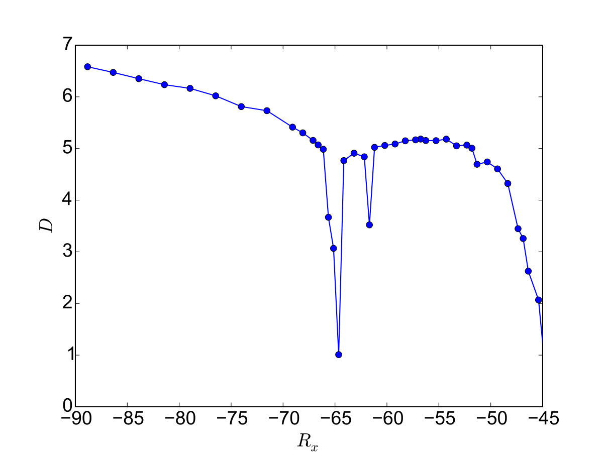 Figure 1
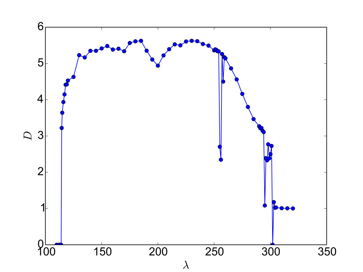 Figure 2
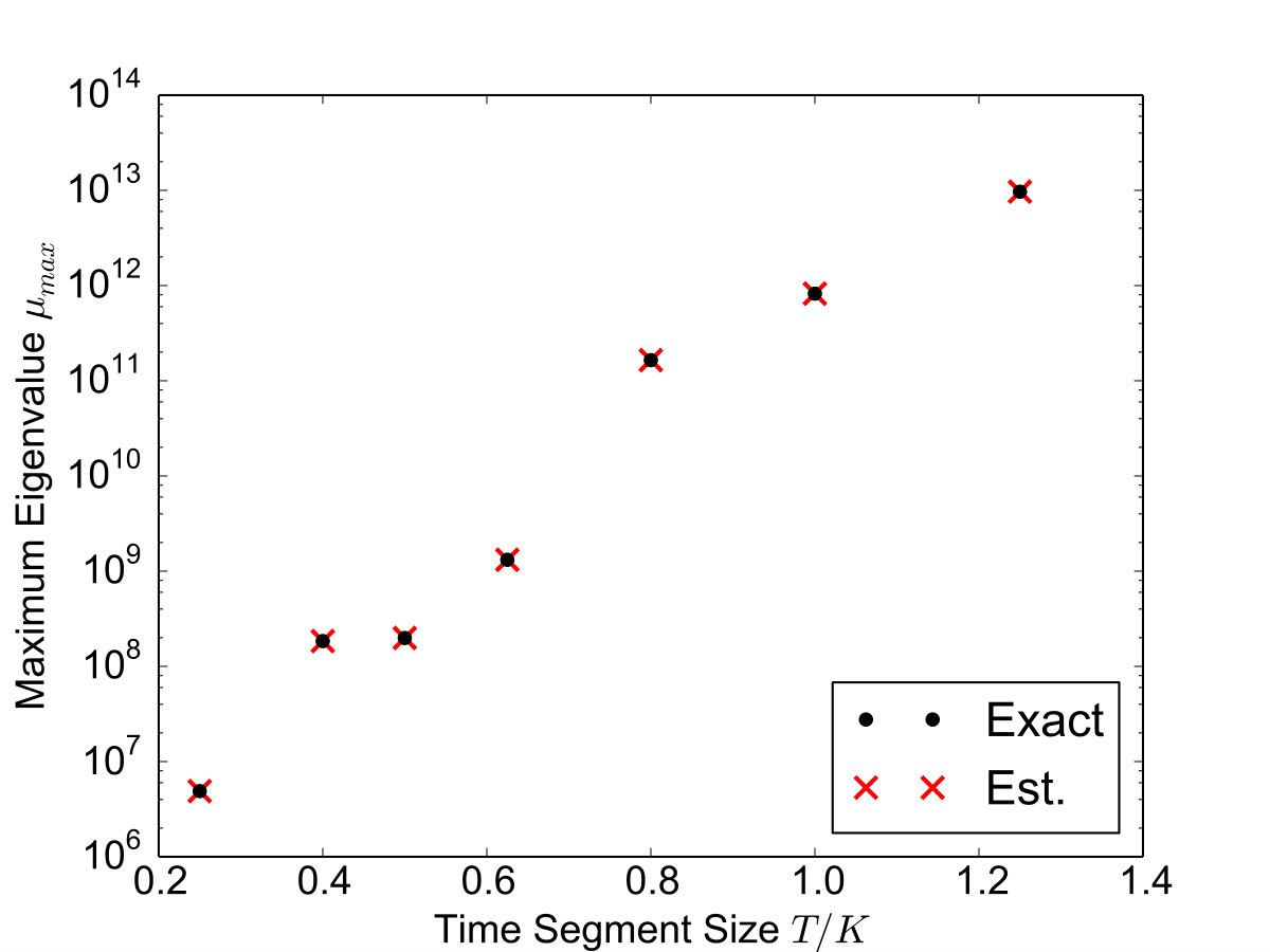 Figure 3
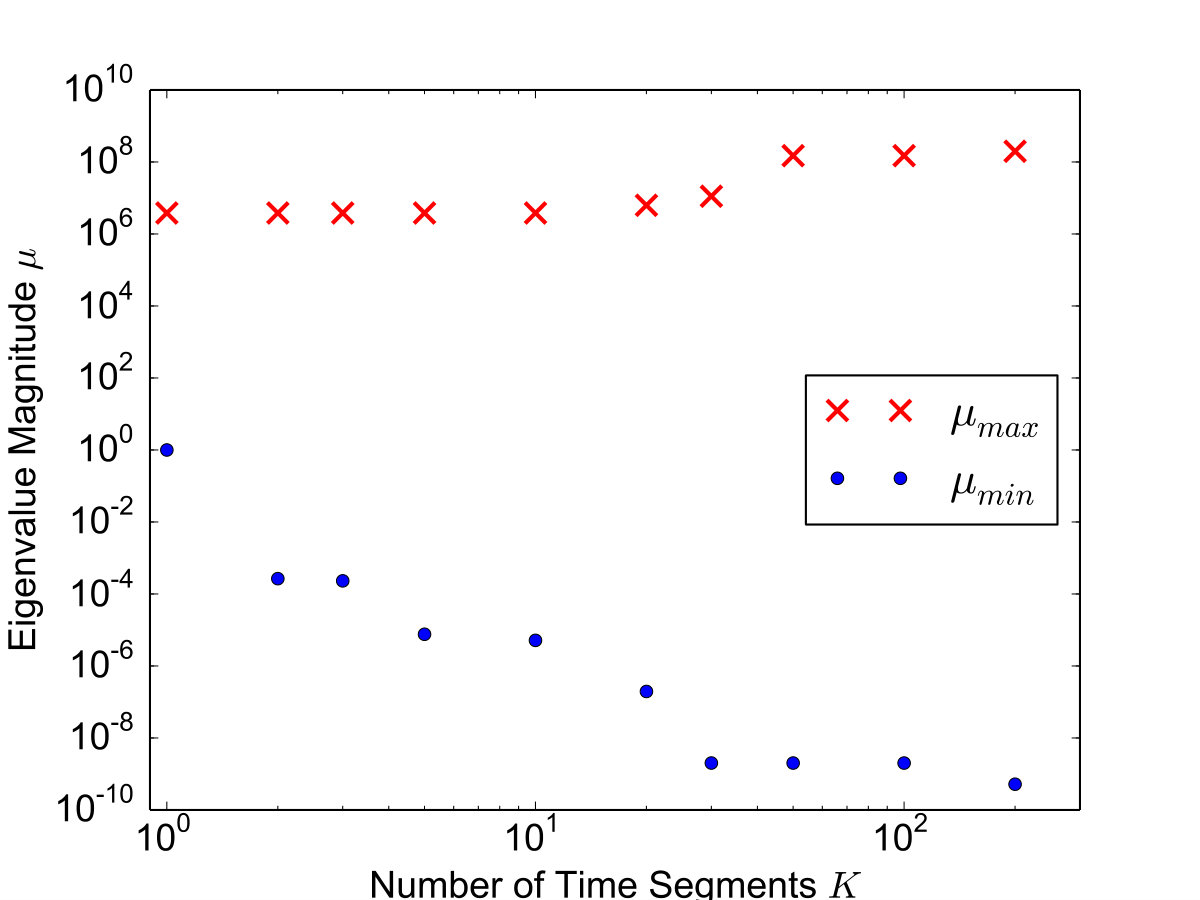 Figure 4
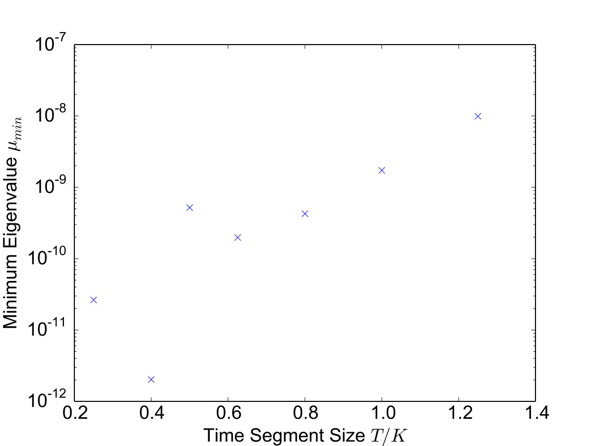 Figure 5
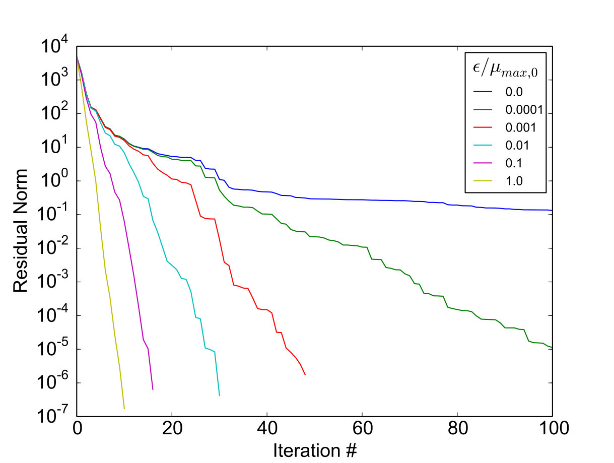 Figure 6
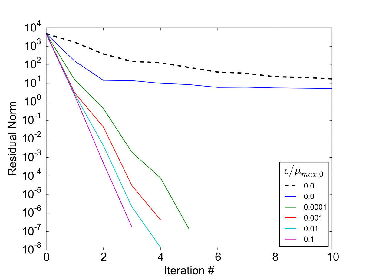 Figure 7
 Figure 8
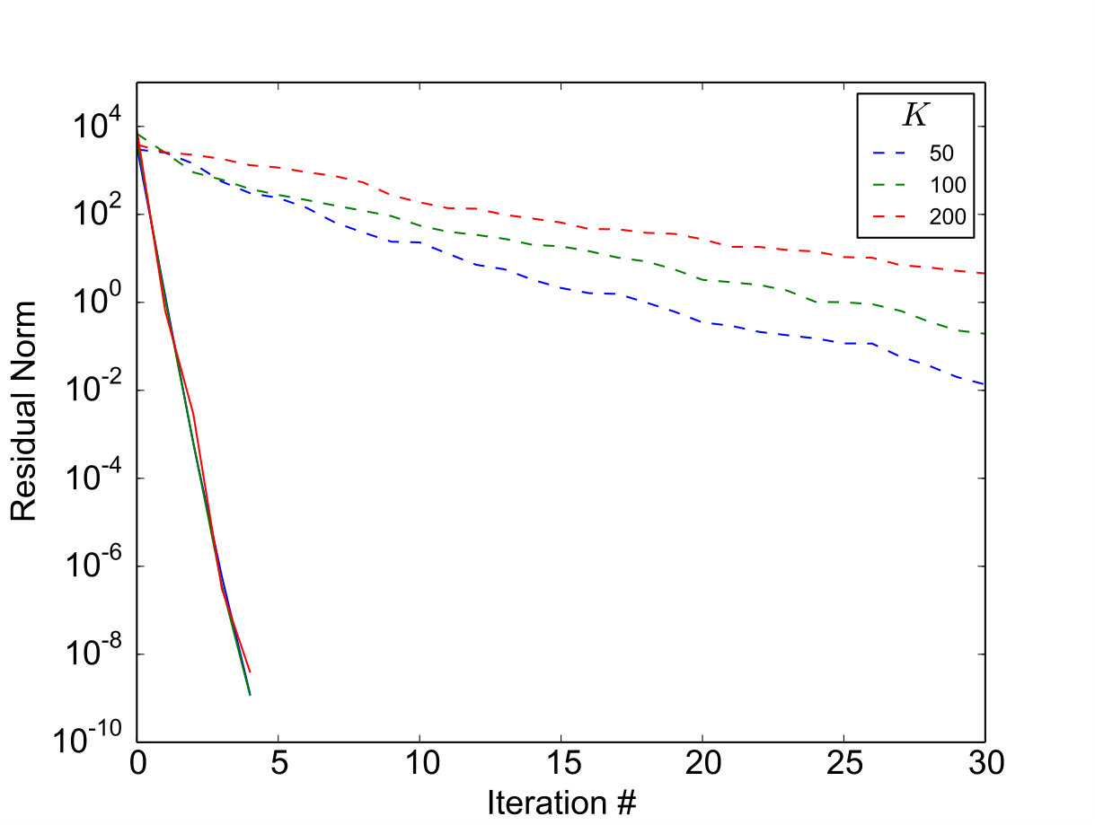 Figure 9
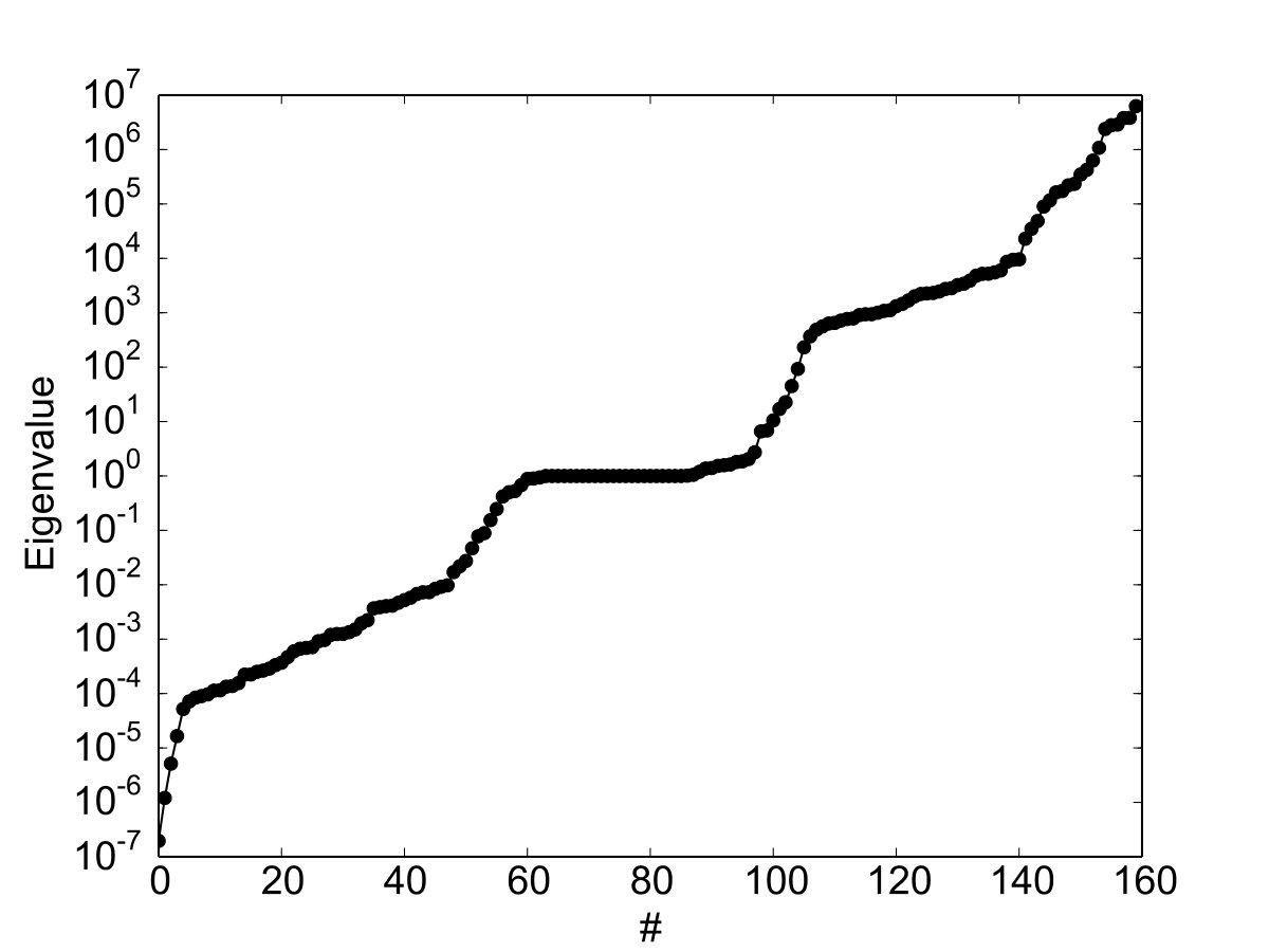 Figure 10
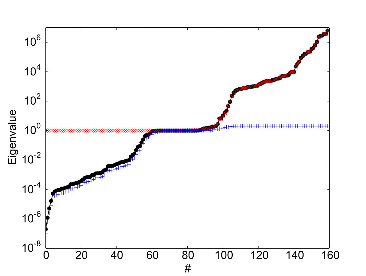 Figure 11
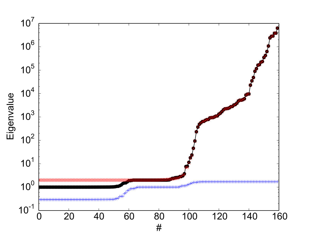 Figure 12
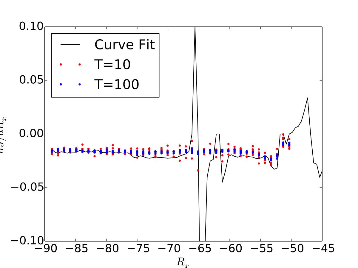 Figure 13
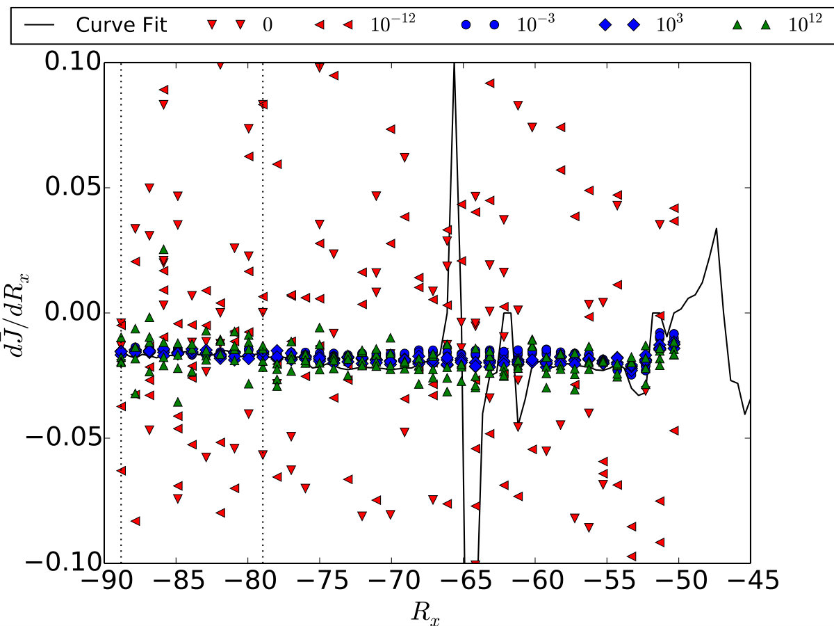 Figure 14
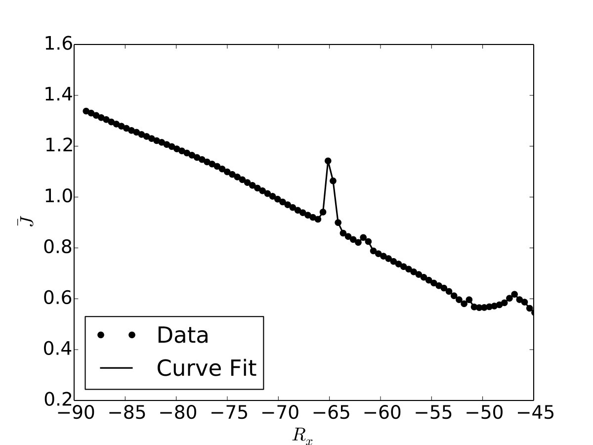 Figure 15
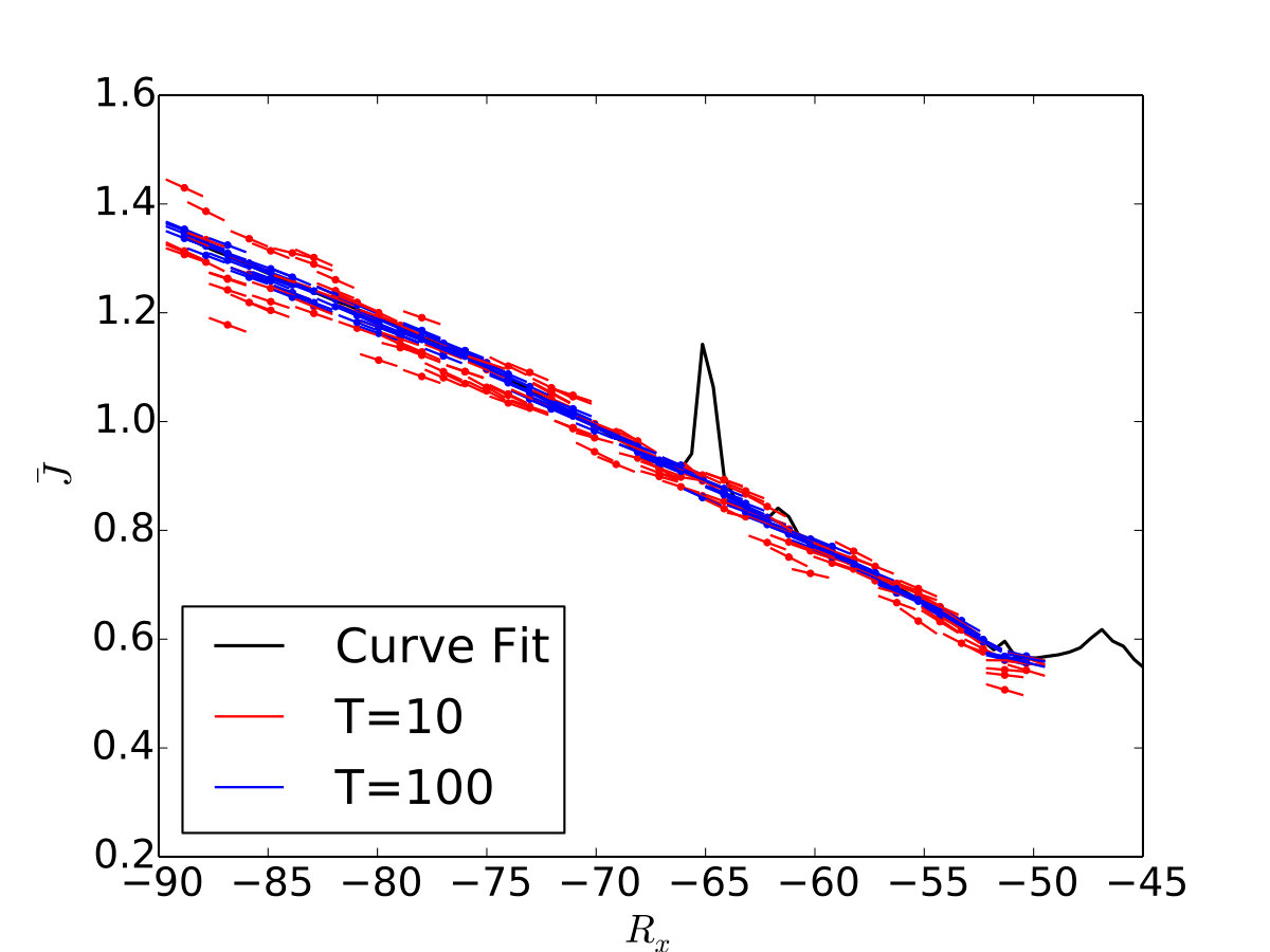 Figure 16
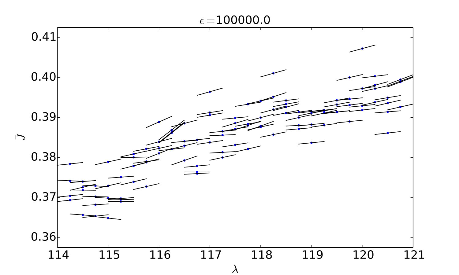 Figure 17
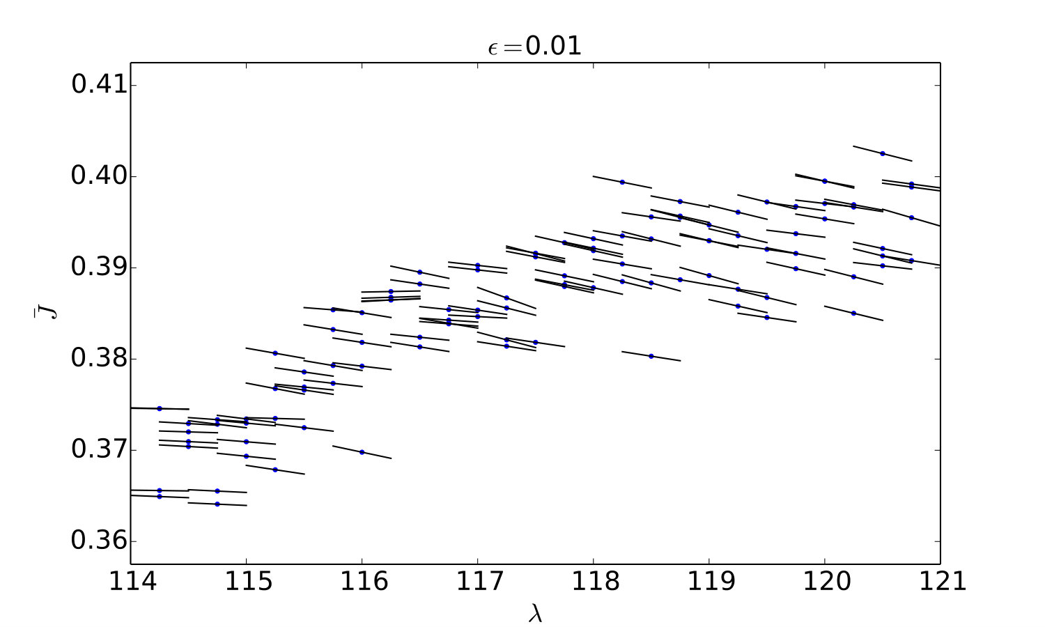 Figure 18
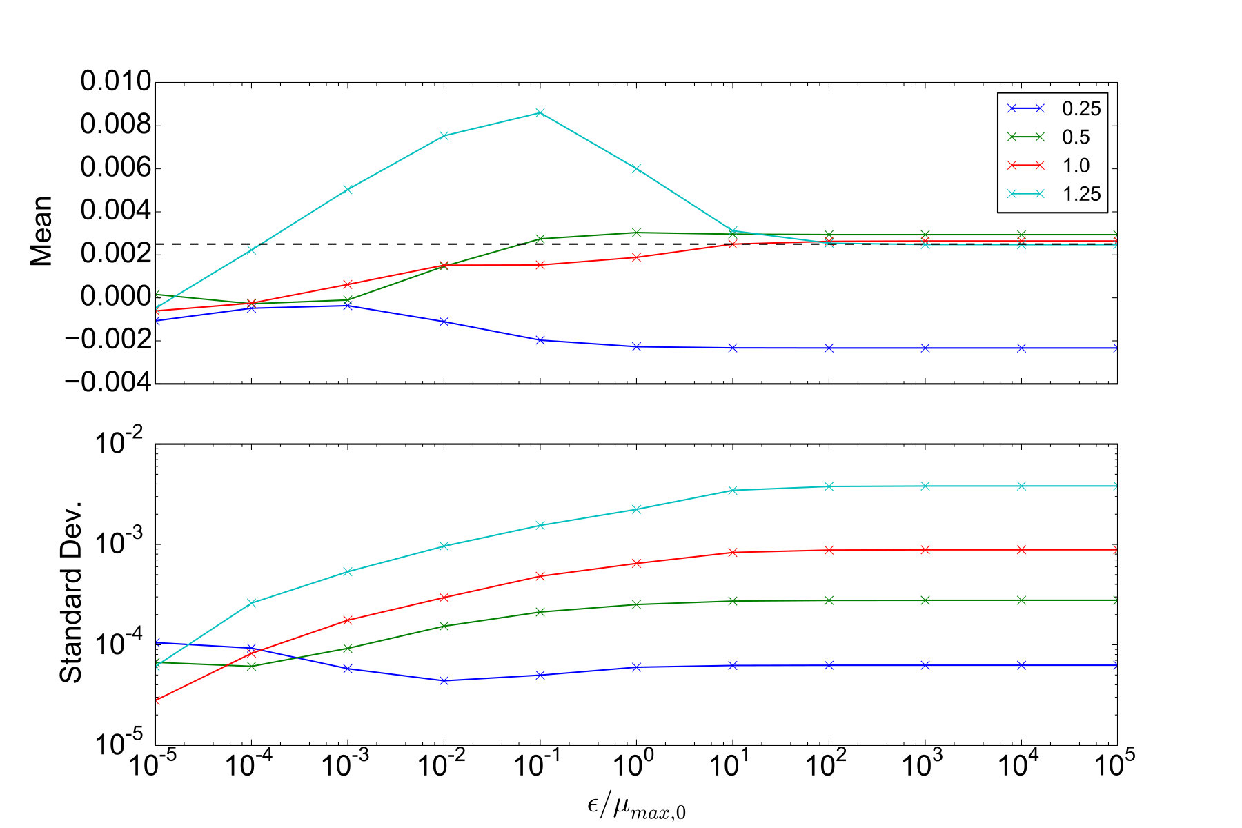 Figure 19
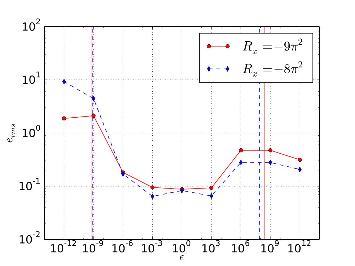 Figure 20
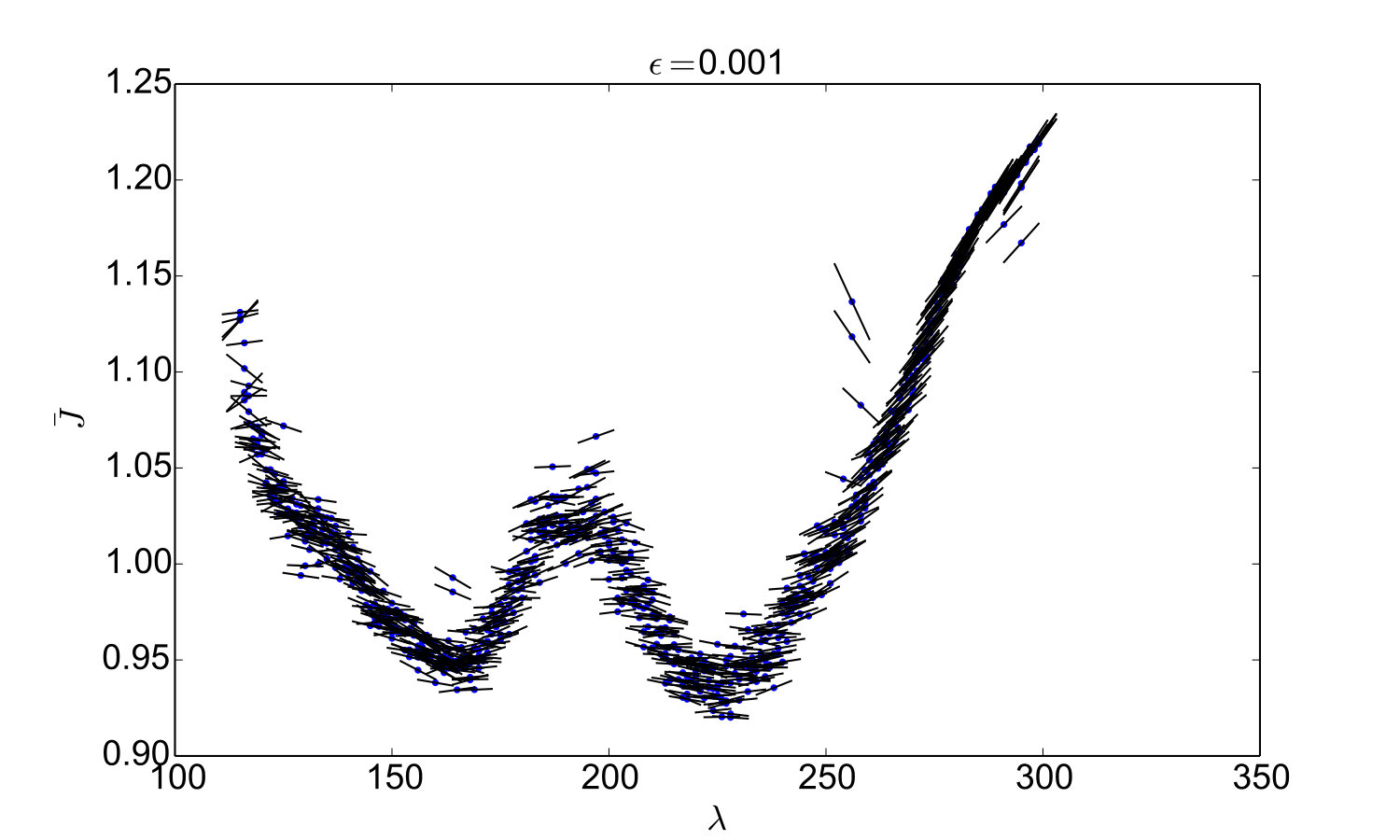 Figure 21
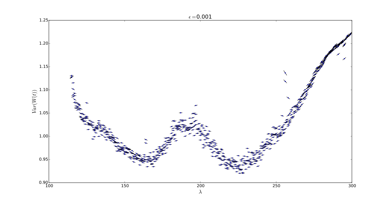 Figure 22
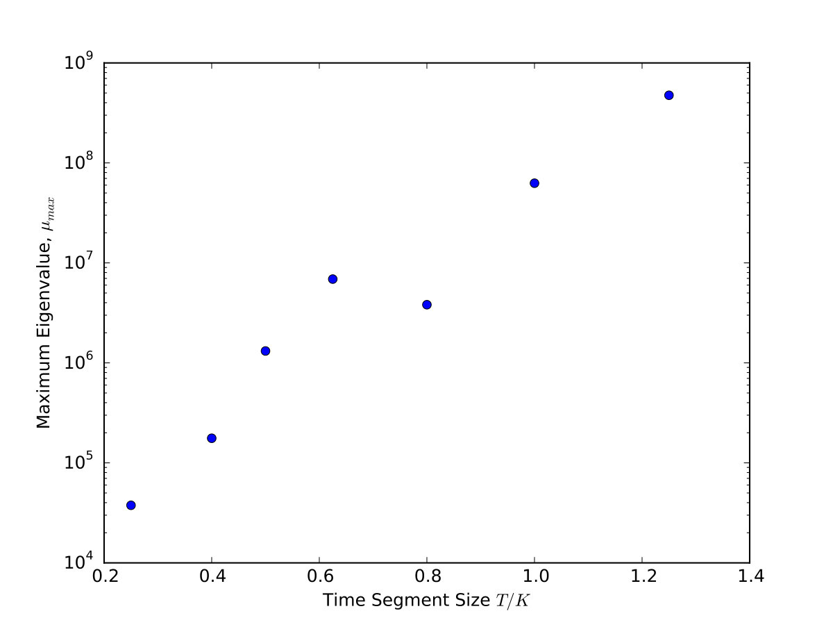 Figure 23
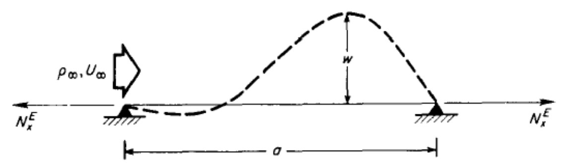 Figure 24
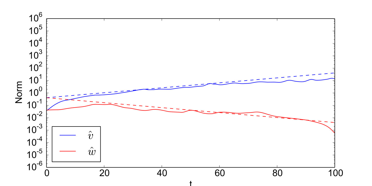 Figure 25
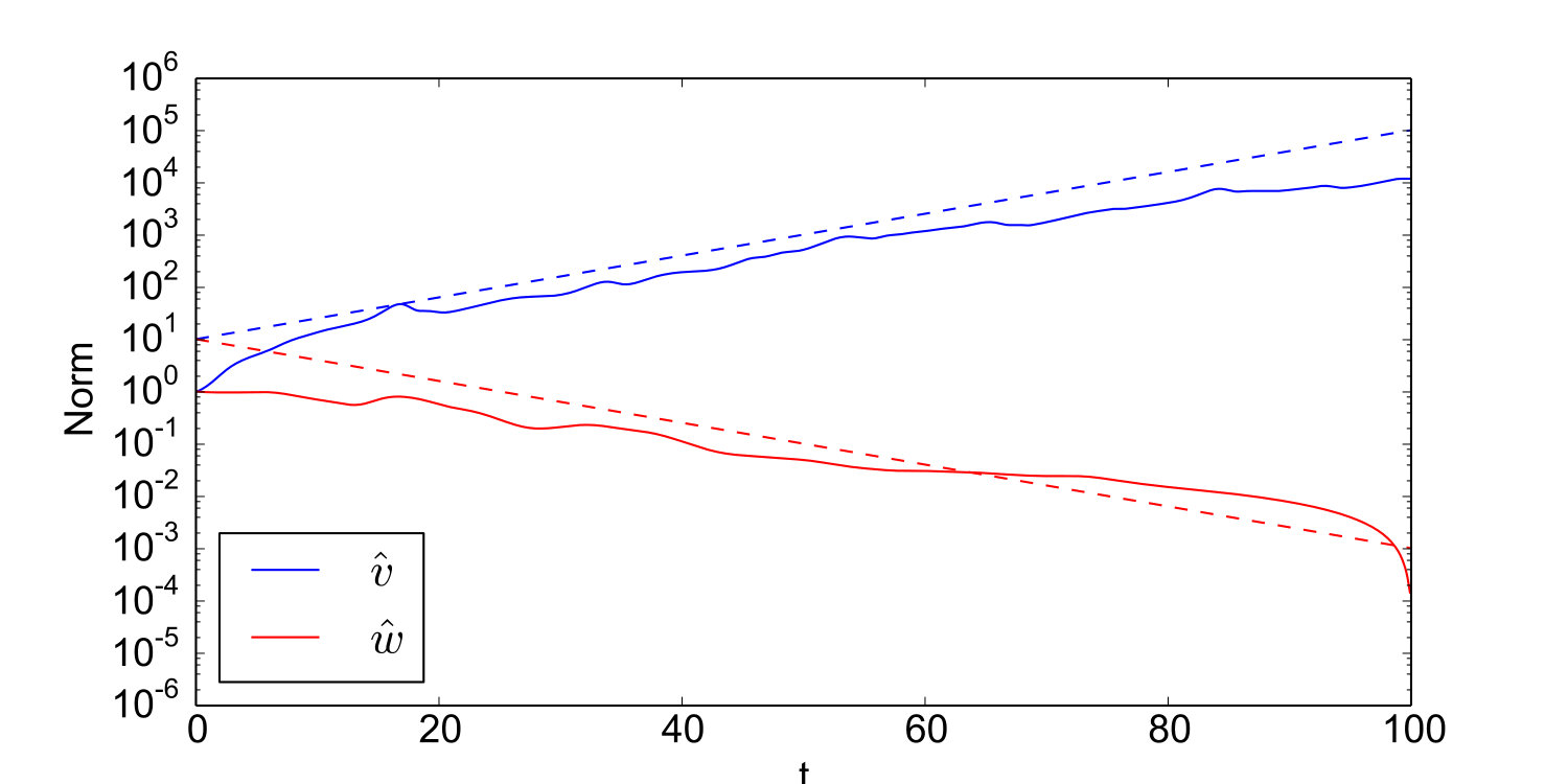 Figure 26
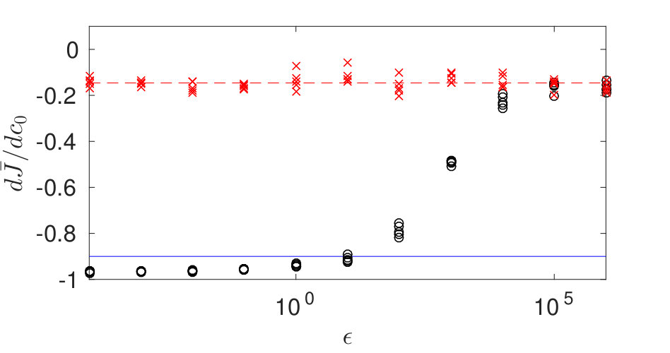 Figure 27
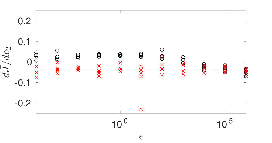 Figure 28
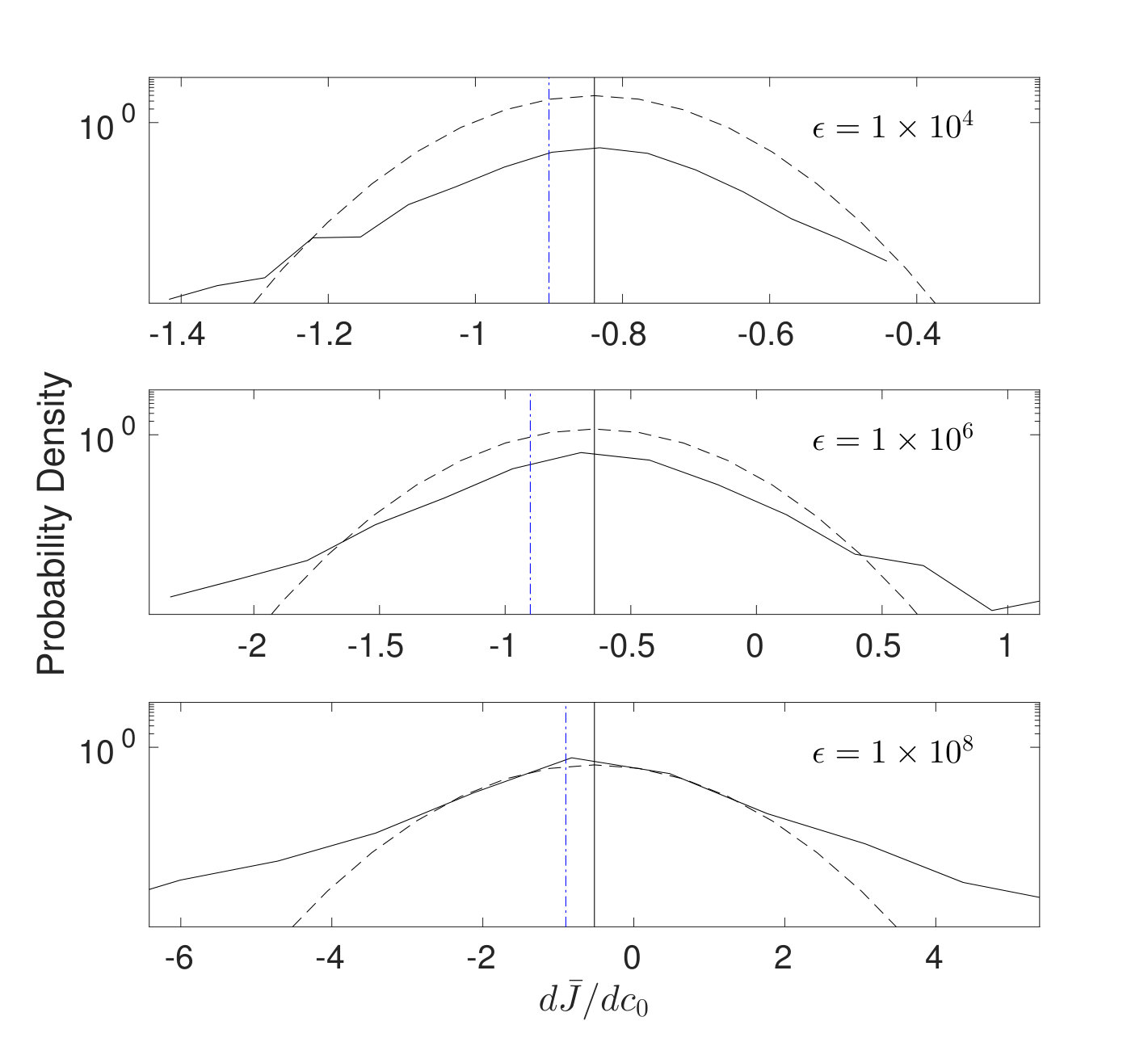 Figure 29
 Figure 30
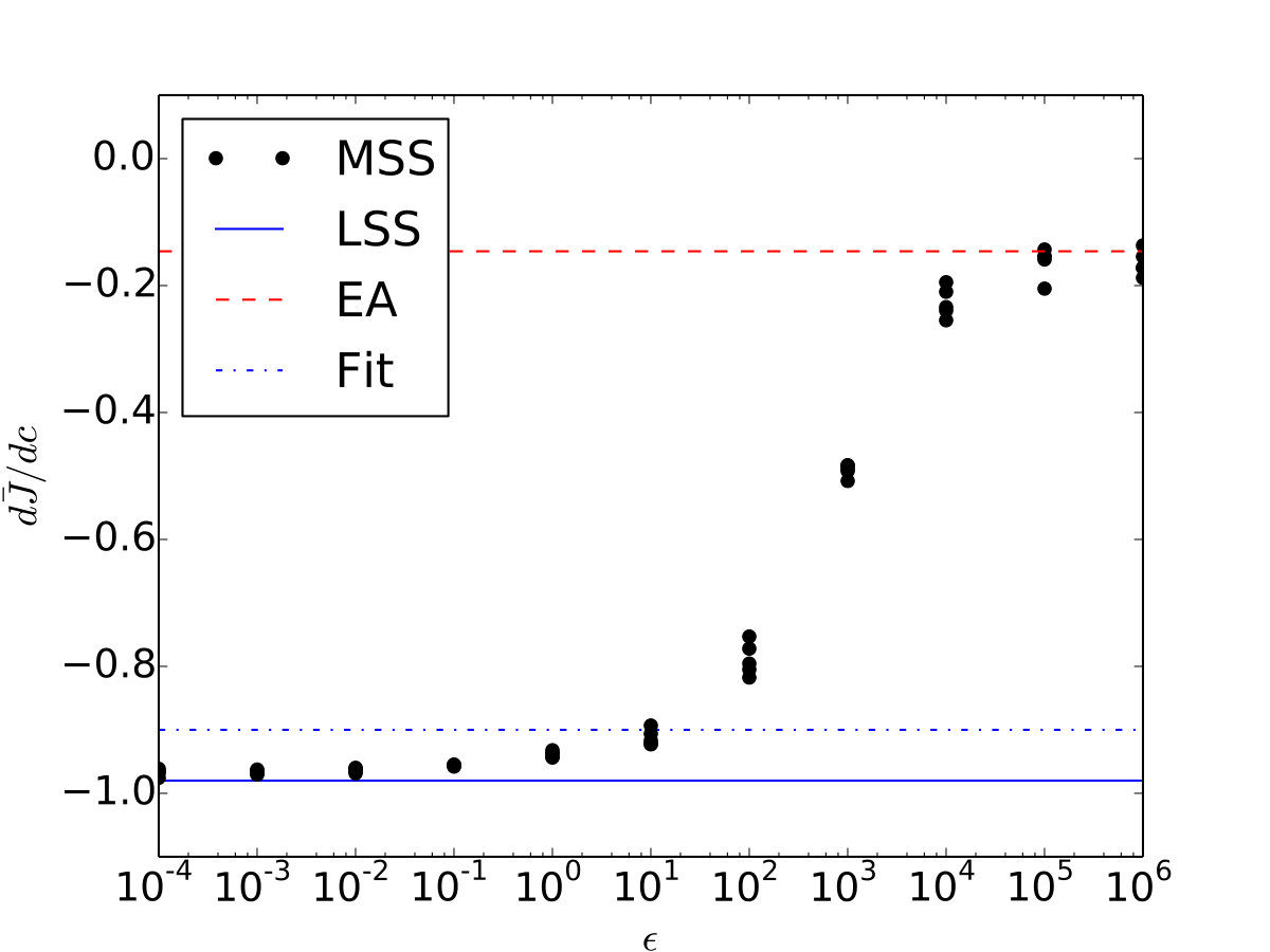 Figure 31
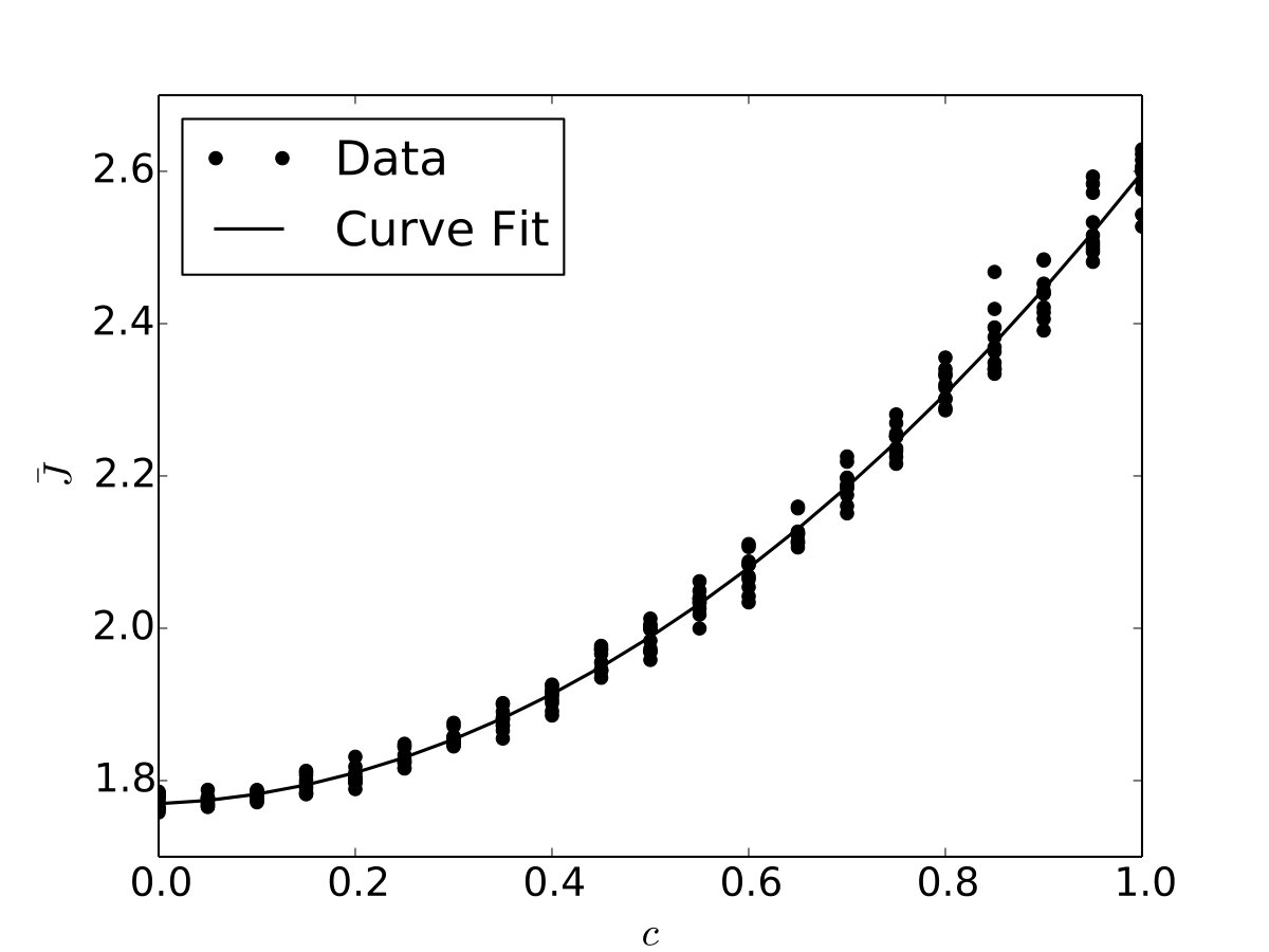 Figure 32
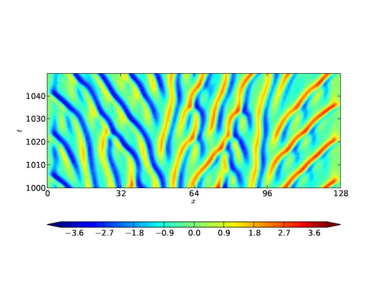 Figure 33
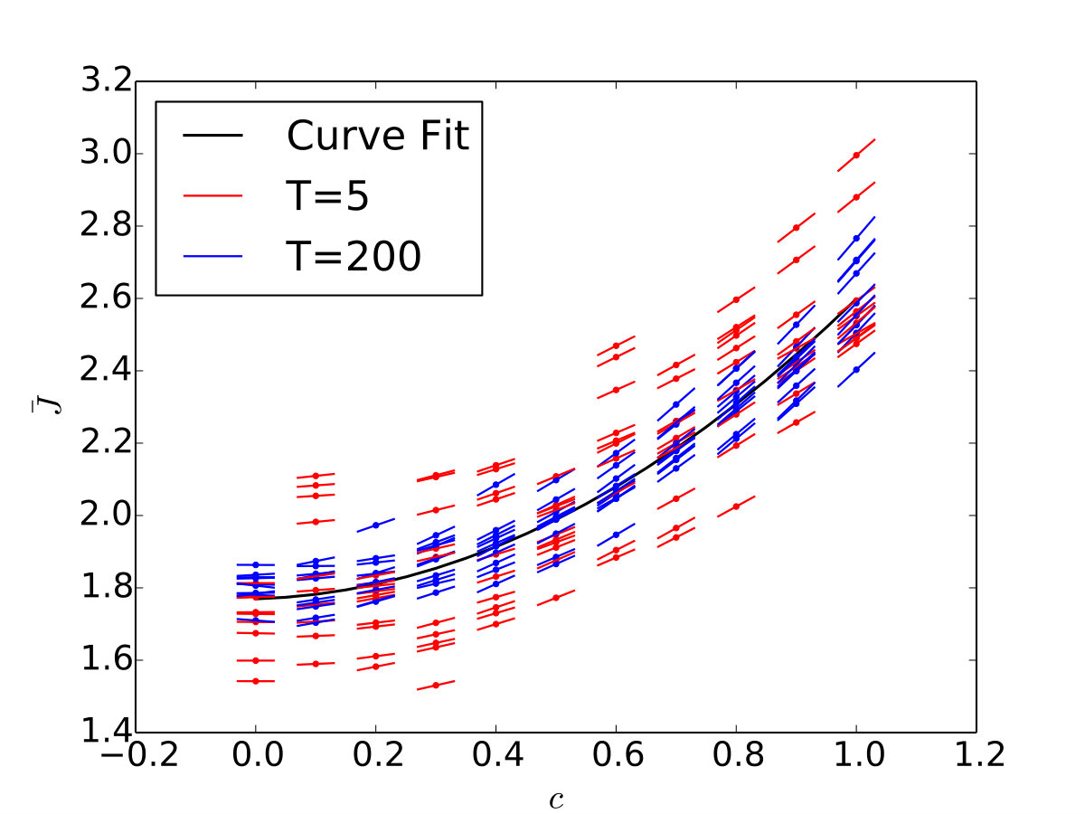 Figure 34
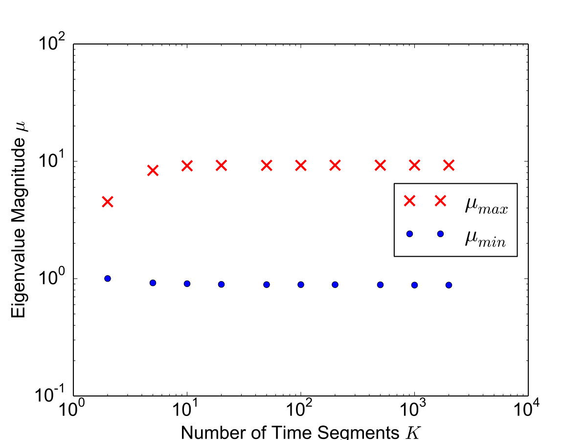 Figure 35
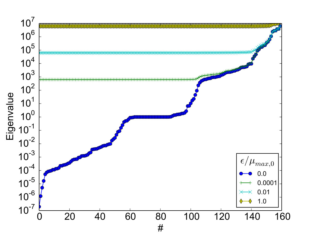 Figure 36
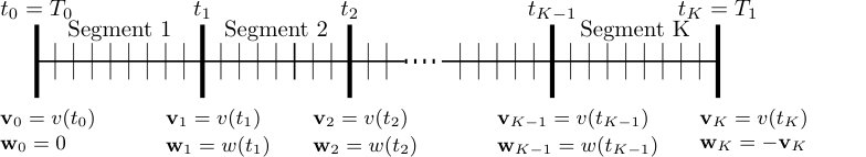 Figure 37
| Variable | Definition |
|---|---|
| plate transverse deflection | |
| streamwise spatial coordinate | |
| time | |
| plate length | |
| plate thickness | |
| mass per unit length of the plate | |
| externally applied in-plane load (positive in tension) | |
| modulus of elasticity | |
| Poisson ratio of the plate material | |
| plate bending stiffness | |
| the tension created by the stretching of the plate due to bending | |
| fluid mass density | |
| flow velocity | |
| flow mach number | |
| static pressure difference across the plate |
Peer Reviews
No public reviews on file for this paper yet. If you reviewed it on a platform where reviews are public (OpenReview, ICLR, NeurIPS, ICML), you can paste yours below so the community can read it here.
Videos
No videos yet. Explain this paper in a talk, walkthrough, or lecture? Add one.
Multiple Shooting Shadowing for Sensitivity Analysis of Chaotic Dynamical Systems
Patrick J. Blonigan111Current Address: NASA Ames Research Center, Moffett Field, CA 94035, United States
Qiqi Wang
Department of Aeronautics and Astronautics, Massachusetts Institute of Technology, 77 Massachusetts Ave, Cambridge, MA 02139, United States
Abstract
Sensitivity analysis methods are important tools for research and design with simulations. Many important simulations exhibit chaotic dynamics, including scale-resolving turbulent fluid flow simulations. Unfortunately, conventional sensitivity analysis methods are unable to compute useful gradient information for long-time-averaged quantities in chaotic dynamical systems. Sensitivity analysis with least squares shadowing (LSS) can compute useful gradient information for a number of chaotic systems, including simulations of chaotic vortex shedding and homogeneous isotropic turbulence. However, this gradient information comes at a very high computational cost. This paper presents multiple shooting shadowing (MSS), a more computationally efficient shadowing approach than the original LSS approach. Through an analysis of the convergence rate of MSS, it is shown that MSS can have lower memory usage and run time than LSS.
keywords:
Sensitivity Analysis , Adjoint , Chaos , Shadowing
††journal: Journal of Computational Physics
1 Introduction
Computational methods for sensitivity analysis are invaluable tools for research and design in many engineering and scientific fields. These methods compute derivatives of outputs with respect to inputs in computer simulations. In applications with large amounts of parameters and only a few important outputs, adjoint-based sensitivity analysis is especially efficient [1]. In aircraft design, for example, the number of geometric parameters that define the outer mold line is typically very large, but engineers may only be interested in a few outputs, such as the lift-to-drag ratio. As a result, the adjoint method of sensitivity analysis has proven to be very successful for aircraft design with gradient-based optimization [2, 3, 4]. The adjoint method has also been an essential tool for adaptive grid methods for solving partial differential equations (PDE’s) [5], error estimation [6], and flow control problems [7]. Finally, some techniques for uncertainty quantification can benefit immensely from sensitivity information [8, 9].
Unfortunately, conventional sensitivity analysis methods, including the adjoint method, can break down when applied to chaotic systems. This occurs for sensitivities of long-time-averaged quantities of interest to design inputs. In this context “long-time” refers to time averaging horizons much larger than the physical time scales associated with the chaotic system being considered. This is problematic, as many key scientific and engineering quantities of interest in chaotic systems are long-time-averaged quantities, such as the time-averaged lift or drag coefficient of a flight vehicle in a high-lift configuration or the average heat transfer to a turbine blade.
To carry out efficient design and analysis of chaotic systems and fluid flows, a new sensitivity analysis method is needed. One promising new approach is Least Squares Shadowing (LSS) [10, 11, 12, 13]. The most common implementation of LSS in the literature is called transcription LSS. Transcription LSS involves solving a globally coupled space-time problem, which can be computationally intensive [10]. The study of LSS for chaotic vortex shedding by Blonigan et al. [14] shows that transcription LSS is very costly in memory usage and operation count for a relatively small simulation. Similar issues with computational cost were encountered in a study of transcription LSS for a direct numerical simulation (DNS) of homogeneous isotropic turbulence [15].
This paper presents an alternative way to pose the minimization statement to compute the shadowing direction or the adjoint shadowing direction. This formulation, multiple shooting shadowing (MSS), addresses the high computational cost of LSS. It is shown that MSS can reduce the memory requirements and the run time required to compute sensitivities of chaotic systems, making LSS sensitivity analysis more tractable for large chaotic dynamical systems such as turbulent fluid flow simulations. The convergence properties of MSS are presented in great detail, along with some approaches to control the convergence rate of MSS.
This paper is organized as follows: section 2 discusses how conventional sensitivity analysis approaches break down for chaotic systems and the past work done to avoid this break down. Section 3 provides an overview of the formulation of transcription LSS. Section 4 introduces the MSS minimization statement and section 5 discusses how MSS can be implemented. Next, section 6 shows MSS results for a chaotic dynamical system and a chaotic partial differential equation (PDE). Section 7 discusses the convergence properties of MSS. Finally, section 8 summarizes this thesis and discusses some future research directions.
2 Sensitivity Analysis of a Chaotic dynamical System
The first question to be asked is if sensitivities are in fact well defined for chaotic systems. It is believed that many, but not every, chaotic system has differentiable time averaged quantities . Specifically, chaotic systems classified as uniformly hyperbolic or quasi-hyperbolic have differentiable time averaged quantities, but non-hyperbolic systems do not. These classes are discussed in greater detail below.
A uniformly hyperbolic attractor is a strange attractor with a tangent space that can be decomposed into stable, neutrally stable, and unstable subspaces at every point in phase space [16]. In other words, the Lyapunov covariant vectors make up a basis for phase space at all points on an attractor. Ruelle’s linear response theorem states that hyperbolic attractors have mean quantities that respond differentiably to small perturbations to their parameters [17]. Therefore, sensitivities are well defined for chaotic systems with hyperbolic attractors. A well studied example of a hyperbolic attractor is the Plykin attractor [18]. The equations governing the Plykin attractor were designed to have hyperbolic properties, which are rare in practice.
Although uniformly hyperbolic attractors are rare, many important properties of hyperbolic systems, including Ruelle’s linear response theorem, can also be shown to hold for the far more common non-uniformly hyperbolic or quasi-hyperbolic attractors [17, 19, 20]. One example of a quasi-hyperbolic attractor is the Lorenz attractor [21]. At the origin of phase space, the Lyapunov covariant vectors for the positive and negative exponent are parallel, so hyperbolicity does not apply. However, this point is an unstable saddle point and almost all phase space trajectories do not pass through it. Because of this the Lorenz attractor appears to have the properties of a hyperbolic attractor, most importantly differentiable mean quantities [22, 10].
Other chaotic dynamical systems have non-hyperbolic attractors. In these non-hyperbolic systems the time averaged quantities are usually not differentiable or even continuous as the parameters vary. In fact, long-time-averages for non-hyperbolic systems may have nontrivial dependence on the initial condition (i.e. the system is not ergodic), which leads to time averaged quantities that are not well-defined.
Fortunately, Gallavotti and Cohen’s chaotic hypothesis conjectures that larger systems behave more like hyperbolic systems than non-hyperbolic systems [23, 24]. That is, larger systems should have differentiable infinite time-averaged quantities. Additionally, a study by Albers and Sprott found that larger chaotic systems tend to have smoothly varying topology changes in the attractor as system parameters are varying [25]. Long-time-averaged quantities do not necessarily vary smoothly across sudden topology changes like bifurcations. Therefore, the chaotic hypothesis and the work by Albers and Sprott suggest there are well defined sensitivities to be computed for a large range of chaotic systems, especially if these systems have a large number of degrees of freedom (DoF). This is encouraging considering the large numbers of DoF’s in simulations such as those of chaotic and turbulent fluid flows.
Additionally, there is some evidence that the chaotic hypothesis applies to simulations of turbulent fluid flows. Grid convergence studies have been done in many cases to ensure that the discretization of the governing equations is sufficiently detailed. For example, Kim et al. used a direct numerical simulation (DNS) to compute turbulent statistics such as the mean velocity profile of a turbulent channel flow with a coarse and a fine spatial discretization [26] to check if their fine discretization was fine enough. The statistics were the same for the coarse and fine discretizations, which shows that long-time-averaged quantities of the DNS respond smoothly to perturbations in the spatial discretization, as predicted by the chaotic hypothesis. Similar results of grid convergence studies for other DNS and Large Eddy Simulation (LES) results [27, 28] also support the chaotic hypothesis, making it very likely that sensitivities of long-time-averaged quantities are well defined for high-fidelity turbulent flow simulations.
2.1 Conventional Sensitivity Analysis
Many time dependent simulations can be interpreted as dynamical systems:
[TABLE]
where is a length vector representing the system state and is a set of design parameters. For a computational fluid dynamics (CFD) simulation, equation (1) represents the discretized Navier-Stokes equations and the state variable is a vector containing the conserved quantities. The design parameters could include geometric parameters for a wing or flow parameters such as the Reynolds number.
When conducting design studies, engineers are typically interested in minimizing some objective function, :
[TABLE]
One example of is the instantaneous drag on an airfoil. For unsteady simulations, time-averaged objective functions are often of interest:
[TABLE]
Sensitivity analysis seeks to compute the derivative of with respect to the design parameters . Traditionally, sensitivity analysis is conducted by solving the following initial value problems
[TABLE]
where is a reference solution and is solution corresponding to a perturbation to some design parameter. Sensitivities can be estimated as:
[TABLE]
However, this initial value problem is very poorly conditioned when the system is chaotic [11]. The “butterfly effect” ensures that and will become decorrelated after some time. This is because when is infinitesimal:
[TABLE]
where is the largest Lyapunov exponent of the system [29] (see A for one way to compute this). Since chaotic dynamical systems have at least one positive Lyapunov exponent, grows exponentially. Therefore, small perturbations to the initial condition or parameter will grow relatively large after a time .
Equation (3) also implies that the linearization will grow exponentially. This growth of is the cause of the following inequality
[TABLE]
or
[TABLE]
Therefore, sensitivity analysis formulated as an initial value problem does not compute useful sensitivities for chaotic dynamical systems. These same issues arise for conventional adjoint sensitivity analysis as well, as shown by Lea et al. for the Lorenz 63 equation [22].
2.2 Chaotic Sensitivity Analysis
Prior work in sensitivity analysis of long-time-averages in chaotic dynamical systems and fluid flows has been done mostly by the climatological and meteorological community. This work includes the ensemble-adjoint method proposed by Lea et al. [22]. This method has been applied to the Lorenz 63 system and an ocean circulation model [30]. Eyink et al. then went on to generalize the ensemble-adjoint method [19]. The ensemble-adjoint method involves averaging over a large number of adjoint calculations for different segments of a time horizon (or time horizons). It was found by Eyink et al. that the sample mean of sensitivities computed with the ensemble adjoint approach for the Lorenz 63 system converges slower than , where is the number of samples, making it less computationally efficient than a naive Monte-Carlo approach [19]. Recently, Ashley and Hicken explored using the ensemble adjoint approach for gradient-based optimization of a chaotic system, but encountered similar issues and observed similarly slow convergence as Eyink et al. [31].
Another idea is the Fokker-Planck adjoint approach for climate sensitivity analysis [32]. This approach involves finding an invariant measure or stationary density which satisfies a Fokker-Planck equation to model the long-time-averaged dynamics, called the “climate” of the system in much of the literature. The adjoint of this Fokker-Planck equation is then used to compute derivatives with respect to long-time-averaged quantities. Fokker-Planck methods typically require discretizing phase space, which limits the method to fairly low dimensional systems. Also many variants of the method require adding diffusion into the system, potentially making the computed sensitivities inaccurate. A Fokker-Planck method proposed by the author and Wang eliminates the need for much of this additional diffusion, but requires a discretization of a manifold approximating the strange attractor, which poses challenges for higher-dimensional, less well understood strange attractors [33].
An analysis based on the Fokker-Planck equation produces the Fluctuation Dissipation Theorem (FDT) [34, 35]. For conservative and nearly conservative dynamical systems, the FDT can be used to accurately compute climate sensitivities [36]. Several improved algorithms based on FDT have since been developed for computing climate sensitivity of non-conservative systems [37, 38, 39]. However, for strongly dissipative systems whose SRB measure [40] deviates strongly from Gaussian, FDT based methods can be inaccurate. Additionally, some of the proposed approaches require computing positive Lyapunov exponents and their corresponding covariant vectors, the current algorithm for which is prohibitively expensive for large systems [38, 41].
3 Transcription Least Squares Shadowing
The poor conditioning of the initial value problem in section 2.1 arises from the problem formulation: and will only be close in phase space at where they share the initial condition ; nothing in the problem formulation requires and to be correlated. LSS overcomes the issues of the initial value problem by minimizing the distance in phase space between and in a least squares sense [10]. This is done by assuming ergodicity and replacing the initial condition with a regularization, as in Doedel and Friedman’s continuation method for computing heteroclinic orbits [42]. This regularization forces and to be as close to one another in phase space as possible for :
[TABLE]
where is a time transformation whose purpose is explained in other LSS literature, and called the time dilation term [10].
LSS uses the assumption of ergodicity to convert an initial value problem to a boundary value problem to improve the conditioning of solving for . The solution to this boundary value problem, , called the “shadow trajectory”, has its existence guaranteed by the shadowing lemma for uniformly hyperbolic systems [43, 44, 10].
To compute sensitivities efficiently, equation (5) is linearized [10]:
[TABLE]
where is called the “shadowing direction”. Equation (6) is a linearly constrained least-squares problem with the following Karush-Kuhn-Tucker (KKT) conditions derived using calculus of variations:
[TABLE]
To compute many sensitivities efficiently, one can derive the adjoint equations for equation (6). Adjoint LSS is derived by Wang et al. [10].
The main approach used to numerically solve for the shadowing direction (or the adjoint shadowing direction) is called transcription LSS. Transcription LSS is when equations (7), (8), and (9) are discretized and solved simultaneously for all time [10]. The KKT system formed by equations (7), (8), and (9) can be reduced to a block tridiagonal linear matrix, where is the number of time steps and is the number of degrees of freedom of the system. The KKT system is solved directly for smaller systems and solved using a multigrid in space and time scheme for larger systems [13, 15].
Transcription LSS has been used to compute accurate sensitivities for a computational fluid dynamics (CFD) simulation of chaotic vortex shedding [14] and a DNS of homogeneous isotropic turbulence [15]. Unfortunately, these studies also show that transcription LSS is very costly in memory usage and operation count. Much of this cost is due to the large size of the KKT system. For example, the chaotic vortex shedding simulation has degrees of freedom. For the time step window considered in the study, the total size of the KKT Schur complement matrix is 22,180,000 rows and roughly 24 GB of input data is required [14]. The system was solved on 2,000 cores for roughly 17 hours to converge the sensitivity to at least 3 decimal places. This high cost provides motivation for the work presented in this paper on the multiple shooting implementation of LSS, called Multiple Shooting Shadowing (MSS).
4 Multiple Shooting Shadowing Formulation
The cost of LSS can be reduced by reformulating the least squares minimization problem (6). More specifically, the objective function in equation (6) can be modified to reduce the number of constraint equations needed to compute a shadowing direction . Instead of minimizing the integral of over a time horizon as in transcription LSS (6), MSS seeks to minimize at discrete checkpoints in time.
[TABLE]
Define time segment as the time span , as shown in figure 1. The MSS minimization problem penalizes large values of at the end of each time segment. By doing this MSS seeks to find that does not grow exponentially over each time segment.
Equation (11) shows that MSS has constraint equations for an -DoF system, compared to for transcription LSS, where is the number of time steps used to discretize the time horizon being studied. Since can be smaller than , the MSS minimization problem can be smaller than that for transcription LSS. In fact, the number of time segments will almost always be smaller than then total number of time steps . This is because the values of and are limited in different ways. If a time segment is too large, will grow too large between checkpoints and round-off errors will impact the accuracy of MSS. The growth rate of is at most the largest Lyapunov exponent . This means that should be used to determine the minimum value of for a fixed time horizon. The number of time steps, is fixed by the desired temporal accuracy and the stability requirements of the time stepping scheme being used. Typically, the time step size needed for stability and accuracy is less than the time needed for round-off errors in the tangent solution to grow to , so . In fact, can be much smaller than when the discretization of the governing equation (1) is stiff or the time accuracy requirements are strict. For example, for the Dowell’s plate model presented later in this chapter, for a relatively large choice of .
The constraint equation (11) enforces continuity at each checkpoint, which forces to satisfy the tangent governing equation (12). Equation (13) fixes to eliminate any component of parallel to . In other words, equations (12) and (13) combine to form a well-defined algebraic-differential equation, in which contains the differential variables and is the algebraic variable.
Before proceeding to derive an expression for , it is useful to define the tangent propagator
[TABLE]
where the superscript indicates an adjoint or transpose operator. The tangent propagator can be used to write the solution to equations (12) as
[TABLE]
The tangent solution from equation (15) will satisfy (12) for any . For to also satisfy equation (13), must satisfy the following closed form expression derived from equations (15) and (13)
[TABLE]
where
[TABLE]
Equation (16) and the above definition of can then be substituted into equation (15) to eliminate
[TABLE]
Therefore, the tangent solution can be made to satisfy (13) by using the projection operator
[TABLE]
To derive the MSS KKT system, equations (15) and (17) are substituted into equations (10) and(11):
[TABLE]
where .
For a dynamical system with degrees of freedom, (19) can be written as
[TABLE]
where is an matrix called the tangent transition matrix and
[TABLE]
is a vector.
All discretized constraints (20) can be written as a system of equations:
[TABLE]
where
[TABLE]
The block matrix is by . The vectors , , and are length , , and , respectively.
Using this notation, equation (10) can be rewritten as
[TABLE]
Next a Lagrangian is formed for equations (23) and (22).
[TABLE]
This Lagrangian is differentiated with respect to and the Lagrange multiplier to obtain the KKT equations
[TABLE]
Together, the KKT equations form a system of equations that can be solved for and :
[TABLE]
As for transcription LSS, the Schur complement of equation (24) is solved instead of the larger full KKT system. The KKT Schur complement for tangent MSS is
[TABLE]
or
[TABLE]
In practice, the matrix is never formed, since each is a dense matrix and is expensive to compute. Instead, a routine for the product is implemented and an iterative method is used to solve (25), as shown in section 5.
Although the matrix is never formed, its structure reveals some key attributes of MSS. From equations (25) and (26), it can be seen that the Schur complement matrix is a , symmetric positive definite and block tridiagonal matrix. As stated previously, is typically much smaller than the total number of time steps . Therefore, the MSS KKT Schur complement is potentially much smaller than the KKT Schur complement for transcription LSS.
Additionally, the structure of the MSS KKT Schur complement is independent of the time discretization used. This is different from transcription LSS, for which the structure of the KKT matrix system depends on the time discretization used [10]. The second order Crank-Nicolson scheme considered by Wang et al. [10] leads to a tridiagonal KKT Schur complement, but higher order time discretizations will lead to more bands in the KKT Schur complement matrix. Therefore MSS has a smaller KKT matrix and possibly also a smaller bandwidth than transcription LSS for a given time horizon and time discretization. This can lead to gains in computational efficiency and a potentially simpler implementation, as shown in section 5.
It should be noted that as , the MSS minimization problem with uniform time segments becomes equivalent to the transcription LSS minimization problem (6) for , where is the weighting parameter in (6). This is explained in more detail in appendix B.
It should be also be noted that the block structure of equation (25) is similar to the LSS KKT system derived for maps [44]. This is because the operator can be thought of as a Jacobian of a nonlinear mapping of from to . For MSS, the nonlinear mapping is solving for from .
As for transcription LSS, the sensitivity of a time-averaged objective function is computed using the following expression [10]
[TABLE]
for an averaging window from to and . The sensitivity of to can be written as a function of from equation (17) (see appendix C for the derivation of the second term)
[TABLE]
where and .
4.1 The Filtering Parameter
The MSS minimization problem expressed by equation (10) and (11) can be modified as follows for a better conditioned KKT system
[TABLE]
where and , as shown in figure 1, and is called the filtering parameter. Equation (29) shows that non-zero values of , create a discontinuous jump of in at the checkpoints . In other words, non-zero values of relax the continuity constraint (11). This has a major impact on the computational efficiency of MSS that will discussed in more detail in section 7.
To derive the KKT equation for MSS with a non-zero , start by rewriting equations (28) in the notation of equation (22)
[TABLE]
and (29) as
[TABLE]
where is a length- vector
[TABLE]
The constraint equation (31) can be used to eliminate from equation (30)
[TABLE]
As is a quadratic function, it is convex, so the minimum of satisfies the first order optimality condition:
[TABLE]
Using equation (31), this expression can be rewritten as
[TABLE]
Together, equations (31) and (33) form a system of equations that can be solved for and :
[TABLE]
Finally, the KKT Schur complement for tangent MSS with non-zero is
[TABLE]
Note that the left-hand side is identical to that of equation (25) with times the identity matrix added on. In section 7 it is shown that this additional term improves the conditioning of (35), allowing iterative solvers to converge to a solution in less time as is increased.
4.2 Adjoint Formulation
When the sensitivities of one time-averaged objective function to many design parameters are desired, adjoint MSS can be used. Adjoint MSS is the discretely consistent adjoint of tangent MSS and can be expressed as the solution of the following linear system, (see appendix D):
[TABLE]
where is a vector and
[TABLE]
The adjoint equations (36) and (37) are derived algorithmically from equations (35) and (27) follwing the discrete adjoint approach as shown in appendix D. Note that the matrix on the left hand side of equation (36) is the same as the one for the tangent MSS KKT Schur complement (35). This is because the matrix is symmetric, and a symmetric matrix is self adjoint.
The sensitivities of can be computed from the adjoint solution with the following expression
[TABLE]
where
[TABLE]
or, in differential equation form
[TABLE]
This can derived by using equation (21), as shown in appendix D.
Interestingly, the adjoint MSS KKT Schur complement (36) is a solution of the following minimization problem
[TABLE]
This is called a ridge regression, or Tikhonov regularization of
[TABLE]
or, equivalently
[TABLE]
this can also be written as
[TABLE]
This shows that equation (42) can be interpreted as solving the conventional adjoint equation (39) in the time horizon , with the initial and terminal conditions
[TABLE]
As has more rows than columns, equation (42) is over-constrained and can be solved with some kind of regularization. The Tikhonov regularization is easy to analyze because unlike other popular regularizations it has an analytical solution for equation (36), the adjoint MSS KKT Schur complement.
5 Implementation
5.1 Adjoint MSS Algorithm
Like transcription LSS implementations, the MSS implementation is comprised of a solver for the KKT Schur complement and a routine to compute gradients from the tangent or adjoint shadowing direction. For MSS, the KKT Schur complement matrix in equation (35) or (36) is not formed explicitly. Instead, a multiple shooting algorithm is derived for equations (35) or (36). This section presents and discusses the multiple shooting algorithm for carrying out adjoint MSS. This algorithm was used to produce the results presented in this paper. The corresponding tangent MSS algorithm can be found in appendix E.
Adjoint MSS Solver
Inputs: Initial condition for the governing equations , Spin-up time , Specified time horizon and checkpoints , Initial guess for the vector , which contains the adjoint variables at checkpoints to (default value 0);
Ouputs: Sensitivities
Calls: MATVEC algorithm that computes where is a residual vector.
Time integrate the governing equations (1) to compute for the specified time horizon. Save the objective function , it is needed for the right hand side of the linear system (36). 2. 2.
To form the right hand side of the linear system, , use the MATVEC algorithm with and . 3. 3.
Use some iterative algorithm to solve equation (35). To compute the left hand side , use MATVEC with . 4. 4.
Compute the sensitivity using equation (38).
Next, a serial MATVEC algorithm is presented. Note that and refer to the time at checkpoint in time segments and , respectively. For example, is the adjoint solution at checkpoint in time segment .
Serial Adjoint MATVEC Algorithm
Inputs: , a vector of the adjoint variables at checkpoints 1 to ; , a scalar;
Ouputs: , a residual vector
MATVEC computes
For all time segments, compute by integrating backwards in time with the terminal condition . 2. 2.
Save . If , save . 3. 3.
For all time segments, compute by integrating with the initial condition . 4. 4.
For all time segments, compute . If , .
Some details of the above algorithms are discussed below.
5.2 Time Integration for MSS
Steps 1 and 3 of the MATVEC algorithm involve solving an adjoint equation for and a tangent equation for , respectively. The algorithm presented in this paper should work with any type of time integration scheme except multi-step schemes such as Adams-Bashforth and Adams-Moulton schemes. These scheme require multiple time steps for an initial condition, which the MATVEC algorithm presented in this paper does not support. Also, it is recommended that the scheme used for is the discrete adjoint of the scheme used for . Using discretely adjoint time integration schemes for solving the tangent and adjoint in MSS ensures that the matrix represented by the MATVEC algorithm is symmetric.
Additionally, it is recommended that the time integration scheme used for computing is the same as that used for computing the solution to the governing equations . This makes the numerical solutions of and discretely consistent. If the numerical solutions of , , and are all discretely consistent, then verification procedures similar to those used for transcription LSS [14] can be used for MSS. If and are not discretely consistent, but and are computed by solvers with consistent and stable discretizations, then MSS should still compute accurate sensitivities, but the implementation would be more difficult to verify.
It should be noted that a pair of time integration schemes for and derived or computed using automatic differentiation will be discretely adjoint and discretely consistent with the scheme used to compute the governing equation solution .
5.3 Iterative Solver for MSS
The 3rd step of the Adjoint MSS algorithm calls for some iterative solver for equation (36). The implementation used for the results presented in this thesis uses MINRES, a Krylov subspace method for solving symmetric, sparse matrices [45, 46]. Another Krylov subspace method, conjugate gradient (CG), was tried on a few chaotic systems, but it was found to converge slightly slower than MINRES. Krylov subspace methods such as GMRES are also used by Sanchez and Net in their multiple shooting continuation algorithm [47].
Krylov subspace methods are not the only viable methods to solve the adjoint MSS KKT Schur complement (36). Other iterative solvers based on Multigrid-in-time could also be used, for example, Multigrid Reduction Methods (MGRIT) [48, 49, 50]. MGRIT uses a multiple shooting approach to solve PDEs, with coarse time step solutions on each time segment used to accelerate the convergence of a fine time step solution. Since MGRIT and MSS both incorporate multiple shooting, a promising area for future work is the study of MGRIT approaches for MSS.
5.4 Time-Parallel MSS
The MATVEC algorithm presented in section 5.1 computes the adjoint and then the tangent on each time segment in sequence, but the computations of the adjoint and tangent on each segment can also be done in parallel. The MATVEC algorithm presented below is parallel-in-time and has each time segment assigned to one processor.
Time-Parallel Adjoint MATVEC Algorithm
Inputs: , a vector of the adjoint variables at checkpoints 1 to ; , a scalar;
Ouputs: , a residual vector
Parallel MATVEC computes on processors. The th time segment is assigned to processor . Processor requires the quantities and (or the ability to compute them) for .
To start, processor has access to .
On processor , do the following:
Compute by integrating backwards in time with the terminal condition . Meanwhile, if , send to processor . Also, if , receive from processor . 2. 2.
Compute and save . If , save . 3. 3.
Compute by integrating with the initial condition . If , use the initial condition . Meanwhile, if , send to processor . Also, if , receive from processor . 4. 4.
Compute . For , .
Due to the block tridiagonal structure of equation (36), time-parallel MATVEC has a very straightforward processor communication pattern: processor only needs to communicate with processors and . This means that time-parallel MATVEC will scale very well: the time required for time-parallel MATVEC should be roughly the same as that required to solve an adjoint and then a tangent equation over one time segment. For large dynamical systems or for processors with slow connections there might be some additional time needed to complete communication of and . For a fixed time segment size, time-parallel MATVEC is much faster than serial MATVEC for large values of which requires time for adjoint solves, followed by tangent solves. For a fixed time horizon , the run time of the time-parallel MATVEC will decrease if the number of processors increases with .
Note that scaling of a time-parallel MSS solver also depends on the linear solver used for step 3 of the Adjoint MSS solver algorithm. For instance, Krylov subspace solvers like MINRES, GMRES, and Conjugate Gradient require a reduce-all operation to compute dot products of the solution vector and residual [45, 46, 51]. Since reduce-all operations involve communication between all processors and one root processor, they have a negative impact on scaling of the linear solver and therefore MSS.
The scaling of time-parallel MSS also depends on the spectral properties of the KKT system which are discussed in section 7. Assume there are one or more time segments per processor. For a fixed time-segment size and a non-zero value of , the minimum and maximum eigenvalues of the KKT system will be independent of . In this case parallel MSS should scale well if a Krylov solver is used because the condition number will stay the same, so the number of solver iterations should stay the same as well222This assumes the clustering of eigenvalues on the real line does not vary much with . . For a fixed time horizon size and a non-zero value of , the maximum eigenvalue of the KKT system will decrease with , while the minimum eigenvalue will be at least . In this case, parallel MSS will scale well, since the time to run the MATVEC will decrease and a decrease in condition number means than the KKT system will likely need fewer solver iterations to converge. However, one must be careful of the impact of on the accuracy of sensitivities, which is discussed in section 7.3. If parallel MSS may not scale well as the minimum eigenvalue will decrease as increases and the KKT system may require more solver iterations to converge.
Finally, it should be mentioned that additional parallelization is possible for governing equations defined over space, like the Navier-Stokes equation. Space-parallel CFD solvers, such as FUN3D, have been in use for a number of years now. Using a space-parallel tangent and adjoint solver in steps 1 and 3 of time-parallel MATVEC would create a space-time-parallel MATVEC. In this case, “processor ” would actually refer to a group of processors corresponding to the tangent and adjoint solvers in time segment . If MSS is to be extended to very large chaotic dynamical systems such as LES, a space-time-parallel MATVEC will be necessary to make the time-to-solution reasonable. Therefore, a space-time-parallel MATVEC should be investigated in future studies of MSS.
5.5 Memory requirements of MSS
The adjoint MSS solver algorithm can be implemented to make memory requirements more reasonable than those discussed for the transcription LSS implementation used in FUN3D [14]. This implementation required storing the governing equation solution and the linearization matrices, including and , at all times in the time horizon studied.
For MSS, major savings in memory usage could be realized by using checkpointing for the adjoint solver in step 3 of the MATVEC algorithm [8]. Checkpointing allows one to time integrate the adjoint backwards in time without saving the governing equation solution and the linearization matrices. Further memory savings can be achieved by solving the tangent equation for in step 3 simultaneously with the governing equations. Such a scheme would only require storage space for , , and the linearization matrices required for one time step. Both of these strategies allow for relatively low memory usage when computing the solution of the adjoint MSS KKT Schur complement equation (36).
Computing sensitivities using equation (38) could also be made memory efficient by computing the integral
[TABLE]
on the fly as is solved, instead of solving for , storing it, then computing the sensitivities of to different input parameters .
MSS could be implemented by recomputing on the fly while solving for and . This would only require storing primal solutions, one for each time segment. Transcription LSS requires at all time steps discretizing the time horizon . Therefore, MSS will require less memory than transcription LSS since .
Finally, the time-parallel MATVEC presented in section 5.4 allows for using distributed memory as the data needed for each time segment can be stored on different CPU’s.
Overall, the MSS formulation offers many more opportunities to minimize storage requirements than transcription LSS. However, memory efficiency alone does not make an algorithm computationally efficient. The time required to complete an algorithm is even more important in many cases.
6 Examples of MSS
6.1 Dowell’s plate
To study characteristics of the MSS algorithm including speed and accuracy, Dowell’s plate model is studied. This model is a relatively simple aeroelastic test problem first explored by Dowell [52]. The set-up, shown in figure 2, is a plate under a compressive in-plane loading in supersonic crossflow. For certain cases, Dowell observed chaotic flutter of this plate [52].
Using linear piston theory, a non-linear thin plate model, and assuming relatively high Mach numbers, the following PDE is obtained [53, 54, 55]:
[TABLE]
where the variables are defined in table 1.
A set of ordinary differential equations (ODE’s) can be obtained from equation (43) using Galerkin’s method with the modal expansion
[TABLE]
which is consistent with simply supported boundary conditions, at and [52]. This results in the following non-dimensional equations
[TABLE]
where , , , , , , and a prime denotes . Also define for later use. All results presented in this paper use four modes (), which is said to be sufficient by Dowell [52].
The two parameters studied are the flow velocity parameter and the load parameter . As is increased in the absence of external compression (), the plate will flutter. On the other hand, as is increased the plate will buckle. Chaotic behavior is observed with the right combination of and , and occurs due to coupling in the buckling and flutter instabilities [52]. MSS is tested in this chaotic region of parameter space ().
The objective function used for this study is the variance of the dimensionless transverse deflection . Also, all calculations presented for Dowell’s plate use the adjoint version of MSS.
Time integration of the governing and tangent equations was done with a 3rd order explicit Runge-Kutta scheme based on the scheme in chapter 6 of [56],
[TABLE]
where subscript corresponds to the th discrete time step, is the time step size and
[TABLE]
The corresponding dual consistent adjoint time stepping scheme was used for adjoint solver for the reasons discussed in section 5.2. The time step size was selected to ensure stability and accuracy of the scheme, resulting in fairly small time steps for Dowell’s plate, which is modeled by stiff ODE’s.
Figures 3 and 5 show that MSS can compute accurate sensitivities for wide ranges of . Figure 5 shows that MSS is very accurate for , fairly accurate for and , and inaccurate for . The regions where MSS is most inaccurate correspond to values of for which the attractor geometry is rapidly changing with respect to , as shown in figure 5. The rapid drops in attractor dimension around and are in the same region where the accuracy of MSS is degraded. This is consistent with the fact that sensitivity analysis is often ill-posed when attractor topology changes rapidly333Attractor topology changes such as bifurcations are inherently non-linear phenomena, so using using the tangent or adjoint equations to compute perturbations near them is a poor approximation, since the tangent and adjoint are linear. Also, there is no guarantee time-averaged objective functions will vary smoothly near topology changes [17].
As MSS is accurate for a wide range of parameters for Dowell’s plate, this test case is used to study the properties of MSS, including the conditioning of the KKT Schur complement matrix in equation (36).
6.2 Kuramoto-Sivashinsky Equation
The second example is the Kuramoto-Sivashinsky (K-S) equation, a case previously studied with LSS [12]. The K-S equation is a 4th order, chaotic PDE, that can be used to model a number of physical phenomena [59]. Kuramoto derived the equation for angular-phase turbulence for a system of reaction-diffusion equations modeling the Belouzov-Zabotinskii reaction in three spatial dimensions [60, 61]. Sivashinsky also derived the equation to model the evolution of instabilities in a distributed plane flame front [62, 63]. In addition the K-S equation has also been shown to be a model of Poiseuille flow of a film layer on an inclined plane [64]. Numerical studies typically use the 1D version of the K-S equation:
[TABLE]
The term is added to make the system ergodic [12]. The equation was solved on the domain , with the boundary conditions:
[TABLE]
These boundary conditions make the K-S equation ergodic, unlike the periodic boundary conditions used in many studies. A typical solution of the K-S equation from a randomized initial condition is shown in figure 6. The initial condition is randomized as follows: since equation (46) is discretized with a 2nd order central difference scheme, at each node is set to a random number drawn from a uniform distribution between -0.5 and 0.5. Time stepping was conducted with the 3rd order Runge-Kutta scheme from equation (45). A time step size of 0.1 units was used for the results presented in this paper.
The objective function considered for the K-S equation in this paper is averaged over both space and time:
[TABLE]
Figure 7 shows sensitivities of computed by MSS. As for Dowell’s plate, MSS computes accurate sensitivities for the K-S equation, just like LSS [12].
7 Rate of Convergence of MSS
One of the main takeaways from the study of LSS for chaotic vortex shedding is that the transcription LSS implementation took a long time to compute sensitivities [14]. This was mainly due to the large number of GMRES iterations (or search directions) required to converge the KKT Schur complement enough to obtain a sufficiently accurate sensitivity. To make LSS practical for large systems like those encountered in CFD simulations, convergence needs to be faster.
The convergence rates of a wide range of iterative solvers depends on the condition number of the matrix. For a symmetric positive definite matrix like the MSS Schur complement, the condition number is defined as the ratio between the largest and smallest eigenvalues, and . Typically, is quite large for the KKT Schur complement matrices derived for both transcription LSS and MSS. Figure 10 shows a typical spectrum for the MSS KKT Schur complement with . This matrix has a condition number . Large values of are problematic, because iterative solvers typically converge faster for systems with smaller . This means that it is desirable to have and as close in value as possible. These eigenvalues depend on the chaotic dynamics of the system being analyzed, the number of time segments , the time segment lengths, , and the filtering parameter . The details of the relationship of and to these properties and parameters is presented using some analysis of the MSS KKT Schur complement and some results for MSS applied to Dowell’s plate.
7.1 The Largest Eigenvalue
First, the largest eigenvalue, , is approximately (see F)
[TABLE]
assuming , where is the length of time segment and the quantity is the largest finite time Lyapunov exponent (FTLE) in time segment . It defined as a finite time approximation of the largest Lyapunov exponent and
[TABLE]
The presence of in (48) shows that is linked to the dynamics of the governing equations being studied. It also explains why the magnitude of is typically large. For many chaotic dynamical systems, including chaotic fluid flows, it has been observed that FTLE’s can vary widely on a strange attractor [65]. This means that in some time segments will be much larger than , in others, it may even be negative. The former case can lead to large values of even for relatively small time segment lengths .
Figure 10 shows that the estimated value of according to equation (48) matches the true maximum eigenvalue very well. Also, it confirms that increases as the time segment size is increased. This growth in with time segment length is non-uniform because of the variation of the FTLE’s on the regions of strange attractor encompassed by the MSS time horizon. Since the same solution and time horizon is considered for all cases in figure 10, different choices of time segments will compute different FTLE’s. The time segment lengths are uniform, so . Therefore, decreasing could decrease in some cases if the maximum FTLE decreases. However, these decreases are only temporary. As is decreased (and is increased) will approach and will grow exponentially with .
Only uniform time segment lengths are considered in this thesis, but the variation of and its impact on may justify using non-uniform time segment lengths for MSS. Non-uniform time segment lengths could be used to control and perhaps even the condition number , depending on how non-uniform time segments impact the smallest eigenvalue .
7.2 The Smallest Eigenvalue
When LSS is conducted for a long enough time horizon, the KKT system for both MSS and transcription LSS can become nearly rank deficient, or .444This is the case for MSS when the filtering parameter is 0. This issue was first observed for early applications of shadowing for noise control [66], but can arise for LSS as well, as shown by the very low values of in figure 10. Also the slow convergence of the KKT Schur complement system for the chaotic vortex shedding case studied by Blonigan et al. [14] suggests the Schur complement is nearly rank deficient.
The small magnitude of when is a symptom of applying LSS or any shadowing approach to a system with a quasi-hyperbolic attractor as opposed to a uniformly hyperbolic attractor. In fact, it has been shown that has a lower bound for uniformly hyperbolic attractors [11]. As discussed in section 2, quasi-hyperbolic attractors include some points where some of the Lyapunov covariant vectors become parallel, called homoclinic tangencies [66]. When a trajectory passes very close to a homoclinic tangency, it is difficult to find corresponding shadow trajectories and therefore, shadowing directions [66].
To understand the difficulty of finding shadowing directions near homoclinic tangencies, consider the th checkpoint for tangent MSS, where . If this checkpoint is on a hyperbolic region of the attractor, then and can be expressed as a linear combination of Lyapunov covariant vectors, which act as a basis for all dimensions of phase space at the point . Define the minimum angle between any two Lyapunov covariant vectors at checkpoint as . In the limit , checkpoint coincides with a homoclinic tangency and two of the covariant vectors are parallel, so now of the covariant vectors are linearly independent. Therefore (and therefore ) can only be expressed a linear combination of covariant vectors. This means there are only degrees of freedom to solve the checkpoint continuity constraint equation (29). Since this is one of the equations that makes up the KKT system, the KKT system is also rank deficient. Therefore small , or equivalently the close proximity of a checkpoint to a homoclinic tangency, implies a low condition number for the entire system.
This is problematic because longer time horizons will increase the likelihood of a checkpoint being close to a homoclinic tangency. This occurs because as a time horizon is increased in length, a solution will pass near more homoclinic tangencies or pass closer by previously visited homoclinic tangencies. This trend was observed for a number of chaotic systems, including Dowell’s plate, which is shown in figure 12. The minimum eigenvalue of the KKT system for Dowell’s plate decreases by orders of magnitude as is increased. On the other hand, the minimum eigenvalue for the uniformly hyperbolic solenoid map shown in figure 12, stays approximately constant as is increased. This behavior is expected since hyperbolic attractors do not have homoclinic tangencies.
Finally, it should be noted that the decrease in the minimum eigenvalue due to homoclinic tangencies also explains the poor conditioning of the transcription LSS KKT system. This is because of the equivalence of MSS for and transcription LSS as shown in section 4 and appendix B.
7.3 Controlling the Condition Number with the Filtering Parameter
The MSS filtering parameter, , can be used to reduce the condition number of the MSS KKT system considerably. It does this by applying a constant shift to the entire eigenvalue spectrum. Define and as the maximum and minimum eigenvalues of the MSS KKT Schur complement with , or . Then the condition number of the MSS KKT Schur complement with non-zero is:
[TABLE]
Given that is typically much smaller than 1 for the MSS KKT Schur complement (see figure 10), a very small value of can improve the condition number by orders of magnitude. This means that non-zero can reduce the number of iterations and therefore the amount of time required by an iterative solver to solve equation (36).
This can be demonstrated on Dowell’s plate. As the MSS system is shown to be nearly indefinite in figure 10, it is solved with the Krylov subspace solver MINRES [45]. Figure 13 shows that increasing results in faster convergence of the residual . At the same time,figures (15) and (15) show that the choice of affects the sensitivities computed by MSS. These figures show that there is an optimal value of between the minimum and maximum eigenvalues and .
Figure (15) shows that the optimal value of is robust and a wide range of produces results with comparable accuracy for Dowell’s plate. The errors when arise because of the poor conditioning of the minimization problem for Dowell’s plate. These errors are not observed for the K-S equation, as shown in figure 16. The errors at large values of observed in figures 15 and 15 arise because adjoint MSS becomes an ensemble adjoint approach as . For large values of , consider equation (36)
[TABLE]
When becomes very large relative to the entries of and , equation (36) becomes
[TABLE]
This corresponds to solving the adjoint in each time segment with a terminal condition of 0, as in the ensemble adjoint method [19]. The only difference is the presence of the projection operator in MSS, but this appears to have a small effect in practice, as seen in figure 16.
The ensemble adjoint method requires a time segment around the size of the largest time scale of the system being analyzed [19]. This time scale is proportional to the largest inverse Lyapunov exponent of the system.
[TABLE]
where is the Lyapunov exponent with the smallest non-zero magnitude. In the case of the modified K-S equation with , this is roughly time units [12]. Since the time segments used for the results in figure 16 are only 102.4 units, MSS suffers from the same bias as the ensemble adjoint. However, lower values of give sensitivities similar to those computed in a previous study [12].
8 Conclusion
Unlike conventional sensitivity analysis methods, LSS is able to compute useful sensitivities of long-time-averaged quantities in chaotic systems. Although other sensitivity analysis methods for chaotic systems have been developed in other communities, these are not viable approaches for high-fidelity, scale-resolving turbulence simulations like LES or DNS. The issues with these other methods include the slow convergence of the ensemble adjoint approach with the number of time horizons used, and the difficulties of extending Fokker-Planck approaches to chaotic systems with many DoFs. LSS avoids many of these issues, but the original implementation of LSS, transcription LSS, suffers from large computational costs.
There are many ways the cost of LSS can be reduced by using multiple shooting rather than a transcription approach. The MSS implementation is definitely more memory efficient than transcription LSS, and can be made to converge faster with the right choice of time checkpoints and filtering parameter. Because of this, larger chaotic dynamical systems like scale-resolving fluid flow simulations should be analyzed with an MSS implementation.
There is still work to be done on the MSS approach itself. This includes exploring other solver approaches such as MGRIT and a detailed investigation of preconditioners for MSS.
Overall, this work is imperative to realizing simulation based design for aerospace vehicles and other engineering devices which require high fidelity flow simulations for accurate analysis. Simulation based design with LSS would be very valuable, leading to gains in performance and providing a deeper understanding of the physics encountered by a wide range of vehicles and devices, from turbomachinery components to heavy-lift launch vehicles.
Appendix A Computing the Maximum Lyapunov Exponent
can be computed by the following approach, a simplification of the algorithm of [41]:
Compute
Inputs: Initial condition for the governing equations , Spin-up time , Specified time horizon and evenly spaced checkpoints with ;
Ouputs: Maximum Lyapunov exponent
Time integrate the governing equations (1) to compute for the specified time horizon. 2. 2.
Set and set equal to some arbitrary unitary vector. 3. 3.
Compute by integrating with the initial condition . 4. 4.
Compute and save . 5. 5.
Set . 6. 6.
Set and repeat steps 3 to 5 until 7. 7.
Solve
[TABLE]
This approximation becomes more accurate as for any choice of . [41]
Appendix B Relationship between MSS and Transcription LSS
For , the LSS minimization problem (6) becomes
[TABLE]
with the KKT equations
[TABLE]
First, for uniformly spaced checkpoints and , the MSS minimization statement multiplied by is
[TABLE]
For and this is equivalent to equation (50). The limit in equation (54) is true because a Riemann sum approaches the Riemann integral as smaller partitions are considered. This also ensures that the second term on the left of (54) disappears as .
The transcription LSS KKT equations are also consistent with the MSS constraint (29). The KKT equations (52) and (53) is equivalent to equations (12) and (13) when and continuity is enforced at checkpoints .
Equations (51) and (52) imply equation (13) holds when . This is because must also hold to ensure that and therefore has no component parallel to and equation (52) is satisfied.
Together, all of this shows that the MSS minimization problem is equivalent to the transcription LSS minimization problem as if the checkpoints are uniformly spaced, and .
Appendix C MSS Gradient
The expression to compute the gradient from and is
[TABLE]
This expression can be written as a function of from equation (17) by using the following expression
[TABLE]
where . Note that
[TABLE]
where , Therefore
[TABLE]
Equation (57) is substituted into equation (55) to obtain
[TABLE]
Finally,
[TABLE]
where .
Appendix D Adjoint MSS Derivation
For a dynamical system with a finite number of states , equation (27) can be rewritten using the notation of equation (34)
[TABLE]
where is a vector and
[TABLE]
Where and . The second term in equation (58) is defined as
[TABLE]
The tangent equation (34) and the sensitivity equation (58) can be combined as follows
[TABLE]
where and are defined as the adjoint variables. Next, rearrange equation (62) as follows
[TABLE]
One can choose and to satisfy the following adjoint equation
[TABLE]
with Schur complement:
[TABLE]
If and satisfy equation (64), then the sensitivities can be computed as follows:
[TABLE]
Using equations (21) and (61), the definitions of and , respectively, equation (66) can be rewritten as:
[TABLE]
From (64):
[TABLE]
For equations (68) and (59) to be true, the adjoint solution in time segment should be
[TABLE]
With this choice of , equation (67) simplifies to:
[TABLE]
Sensitivities of with respect to many parameters can be computed with a single solution of .
Appendix E Tangent MSS Algorithm
Since the adjoint MSS Schur complement (36) is identical to the tangent MSS Schur complement (35) the adjoint and tangent algorithms are very similar:
Tangent MSS Solver
Inputs: Initial condition for the governing equations , Spin-up time , Specified time horizon and checkpoints , Initial guess for vector , which contains the Lagrange multipliers at checkpoints to (default value 0);
Ouputs: Sensitivity
Calls: MATVEC algorithm that computes where is a residual vector.
Time integrate the governing equations (1) to compute for the specified time horizon. 2. 2.
To form the right hand side of the linear system, , use the MATVEC algorithm with and . 3. 3.
Use some iterative algorithm to solve equation (35). To compute the left hand side , use MATVEC with . 4. 4.
Compute the sensitivity using equation (27).
Next, a serial MATVEC algorithm is presented. Note that and refer to the time at checkpoint in time segments and , respectively. For example, is the tangent solution at checkpoint computed in time segment .
Serial Tangent MATVEC Algorithm
Inputs: , a vector of the Lagrange multipliers at checkpoints 1 to ; , a scalar;
Ouputs: , a residual vector
MATVEC computes
For all time segments, compute by integrating backwards in time with the terminal condition . 2. 2.
Save . If , save . 3. 3.
For all time segments, compute by integrating with the initial condition . 4. 4.
For all time segments, compute . If , .
Appendix F Estimating the largest eigenvalue of the MSS KKT Schur complement
The largest eigenvalue of the MSS KKT Schur complement, , is related to the positive Lyapunov exponent discussed in section 2.1. This can be shown with the singular value decomposition (SVD) of the tangent transition matrix defined in equation (20),
[TABLE]
where and are orthonormal matrices and is a diagonal matrix with singular values along the main diagonal. The singular values are indexed in descending order of magnitude, that is .
Interestingly the singular value can be interpreted as a finite time approximation of the largest Lyapunov exponent. The maximum Lyapunov exponent can be defined as [67]
[TABLE]
where is the th singular value of a the tangent propagator , which is a matrix for a system with states. Recall that . The projection operator only removes any component parallel to , which happens to be the Lyapunov covariant vector for the zero Lyapunov exponent. Therefore, has no impact on the covariant vector corresponding to and
[TABLE]
where is the time segment length for segment . Since is defined as the maximum singular value of in equation (82),
[TABLE]
The quantity can be interpreted as a finite time approximation of in time segment . From equation (84), the singular value can be written in terms of the finite time Lyapunov exponent
[TABLE]
Recall from section 7.1 that can be much larger than 1 due to variations in over each time segment. Because of this, it can be assumed that
[TABLE]
if or is sufficiently large.
Next, the connection between and the is considered. Recall from equations (35) and (26) that the MSS Schur complement matrix is a block-tridiagonal matrix with the main block diagonal and and . Therefore, the eigenvalues of must be related to the singular values of . It can be shown that the largest eigenvalue of the is
[TABLE]
To show this, consider the case where the maximum singular value is , corresponding the tangent propagator . Then, for ,
[TABLE]
Rows and of are negligible relative to row if as in equation (86) and .
In row , since by definition ,
[TABLE]
The magnitude of row of is a maximum when , as will be stretched by the largest singular value for time segment , , so
[TABLE]
since is the largest singular value for all time segments, and since by definition
[TABLE]
The inequalities in equations (123) and (124) show that
[TABLE]
Therefore, the largest eigenvalue of is
[TABLE]
with the corresponding eigenvector . Since is by definition the largest singular value for all time segments, equations (126) and (87) are equivalent.
Note that in the typical spectrum shown in figure 10. Since this spectrum was computed for , the assumption is consistent with a typical spectrum of .
Therefore,
[TABLE]
Acknowledgments
Research for this paper was conducted with Government support under FA9550-11-C-0028 and awarded by the Department of Defense, Air Force Office of Scientific Research, National Defense Science and Engineering Graduate (NDSEG) Fellowship, 32 CFR 168a.
References
- [1]
M. Giles, N. Pierce, An introduction to the adjoint approach to design, Flow, Turbulence and Combustion 65 (2000) 393–415.
- [2]
A. Jameson, Aerodynamic design via control theory, Journal of Scientific Computing 3 (3) (1988) 233–260.
- [3]
J. Reuther, A. Jameson, J. J. Alonso, M. J. Rimlinger, D. Sanders, Constrained multipoint aerodynamic shape optimization using an adjoint formulation and parallel computers, Journal of Aircraft 36 (1) (1999) 51–74.
- [4]
J. R. R. A. Martins, J. J. Alonso, J. J. Reuther, A coupled-adjoint sensitivity analysis method for high-fidelity aero-structural design, Optimization and Engineering 6 (1) (2005) 33–62.
http://dx.doi.org/DOI:10.1023/B:OPTE.0000048536.47956.62
- [5]
D. Venditti, D. Darmofal, Grid adaptation for functional outputs: Application to two-dimensional inviscid flow, Journal of Computational Physics 176 (2002) 40–69.
- [6]
M. Giles, E. Süli, Adjoint methods for pdes: a posteriori error analysis and postprocessing by duality, Acta Numerica 11 (2002) 145–236.
- [7]
M. Gunzburger, Perspectives in Flow Control and Optimization, Society for Industrial and Applied Mathematics, Philadelphia, PA, USA, 2002.
- [8]
Q. Wang, Uncertainty quantification for unsteady fluid flow using adjoint-based approaches, PhD dissertation, Stanford University (2009).
- [9]
Q. Wang, K. Duraisamy, J. Alonso, G. Iaccarino, Risk assessment of scramjet unstart using adjoint-based sampling methods, AIAA Journal 50 (3) (2012) 581–592.
- [10]
Q. Wang, R. Hui, P. Blonigan, Least squares shadowing sensitivity analysis of chaotic limit cycle oscillations, Journal of Computational Physics 267 (2014) 210–224.
- [11]
Q. Wang, S. Gomez, P. Blonigan, A. Gregory, E. Qian, Towards scalable parallel-in-time turbulent flow simulations, Physics of Fluids 25.
http://dx.doi.org/10.1063/1.4819390.
- [12]
P. Blonigan, Q. Wang, Least squares shadowing sensitivity analysis of a modified Kuramoto–Sivashinsky equation, Chaos, Solitons, and Fractals 64 (2014) 16–25.
- [13]
P. Blonigan, Q. Wang, Multigrid-in-time for sensitivity analysis of chaotic dynamical systems, Numerical Linear Algebra with Applications 21 (2).
- [14]
P. Blonigan, Q. Wang, E. Nielsen, B. Diskin, Least squares shadowing sensitivity analysis of chaotic flow around a two-dimensional airfoil, AIAA 2016-0296, 2016.
- [15]
S. Gomez, Parallel multigrid for large-scale least squares sensitivity, Master’s thesis, Massachusetts Institute of Technology, Cambridge, MA (2013).
- [16]
B. Hasselblatt, Hyperbolic dynamical systems, in: Handbook of Dynamical Systems 1A, Elsevier, North Holland, 2002, pp. 239–319.
- [17]
D. Ruelle, Differentiation of SRB states, Communications in Mathematical Physics 187 (1997) 227–241.
- [18]
S. Kuznetsov, A non-autonomous flow system with Plykin type attractor, Communications in Nonlinear Science and Numerical Simulation 11 (9) (2009) 3487–3491.
- [19]
G. Eyink, T. Haine, D. Lea, Ruelle’s linear response formula, ensemble adjoint schemes and Lévy flights, Nonlinearity 17 (5) (2004) 1867–1889.
- [20]
C. Bonatti, L. Diaz, M. Viana, Uniform Hyperbolicity: A Global Geometric and Probabilistic Perspective, Springer, 2005.
- [21]
E. Lorenz, Deterministic nonperiodic flow, Journal of the Atmospheric Sciences 20 (1963) 130–141.
- [22]
D. Lea, M. Allen, T. Haine, Sensitivity analysis of the climate of a chaotic system, Tellus 52A (2000) 523–532.
- [23]
G. Gallavotti, E. Cohen, Dynamical ensembles in stationary states, Journal of Statistical Physics 80 (1995) 931–970.
- [24]
G. Gallavotti, E. Cohen, Dynamical ensembles in nonequilibrium statistical mechanics, Physical Review Letters 74 (1995) 2694–2697.
- [25]
D. Albers, J. Sprott, Structural stability and hyperbolicity violation in high-dimensional dynamical systems, Nonlinearity 19 (2006) 1801–1847.
- [26]
J. Kim, P. Moin, R. Moser, Turbulence statistics in fully developed channel flow at low Reynolds number, Journal of Fluid Mechanics 177 (1986) 133–166.
- [27]
G. Medic, J. Joo, S. Lele, O. Sharma, Prediction of heat transfer in a turbine cascade with high levels of free-stream turbulence, in: Proceedings of the 2012 Summer Program, Center for Turbulence Research, Stanford, 2012, pp. 147–155.
- [28]
S. Bose, P. Moin, D. You, Grid-independent large-eddy simulation using explicit filtering, Physics of Fluids 22 (2010) 105103.
- [29]
S. Strogatz, Nonlinear Dynamics and Chaos: With Applications to Physics, Biology, Chemistry, and Engineering, Westview Press, Philadelphia, PA, 1994.
- [30]
D. Lea, T. Haine, M. Allen, J. Hansen, Sensitivity analysis of the climate of a chaotic ocean circulation model, Journal of the Royal Meteorological Society 128 (2002) 2587–2605.
- [31]
A. Ashley, J. Hicken, Low Reynolds number numerical solutions of chaotic flow, in: AIAA Aviation 2014 Symposium on the Theory of Computing, Atlanta, Georgia, United States, 2014, aIAA-2014-2434.
- [32]
J. Thuburn, Climate sensitivities via a Fokker-Planck adjoint approach, Quarterly Journal of the Royal Meteorological Society 131 (605) (2005) 73–93.
- [33]
P. Blonigan, Q. Wang, Probability density adjoint for sensitivity analysis of the mean of chaos, Journal of Computational Physics 270 (2014) 660–686.
- [34]
H. Nyquist,Thermal agitation of electric charge in conductors. Phys. Rev. 32 (1928) 110–113.
http://dx.doi.org/10.1103/PhysRev.32.110.
- [35]
R. Kubo, The fluctuation-dissipation theorem, Reports on Progress in Physics 29 (1) (1966) 255.
- [36]
C. Leith, Climate response and fluctuation dissipation, Journal of the Atmospheric Sciences 32 (10) (1975) 2022–2026.
- [37]
A. Majda, R. Abramov, M. Grote, Information Theory and Stochastics for Multiscale Nonlinear Systems, CRM Monograph Series, American Mathematical Society, 2005.
- [38]
R. Abramov, A. Majda, New approximations and tests of linear fluctuation-response for chaotic nonlinear forced-dissipative dynamical systems, Journal of Nonlinear Science 18 (2008) 303–341.
- [39]
R. Abramov, A. Majda, Blended response algorithms for linear fluctuation-dissipation for complex nonlinear dynamical systems, Nonlinearity 20 (12) (2007) 2793.
- [40]
L.-S. Young,What are SRB measures, and which dynamical systems have them?, Journal of Statistical Physics 108 (5-6) (2002) 733–754.
http://dx.doi.org/10.1023/A:1019762724717.
- [41]
G.Benettin, L. Galgani, A. Giorgilli, J. Strelcyn, Lyapunov characteristic exponents for smooth dynamical systems and for Hamiltonian systems; a method for computing all of them. part 2: Numerical application, Meccanica 15 (1) (1980) 21–30.
- [42]
E. J. Doedel, M. J. Friedman, Numerical computation of heteroclinic orbits, Journal of Computational and Applied Mathematics 26 (1-2) (1989) 155–170.
- [43]
S. Y. Pilyugin, Shadowing in dynamical systems, 1st Edition, Vol. 1706 of Lecture Notes in Mathematics, Springer-Verlag, New York, 1999.
- [44]
Q. Wang, Convergence of the least squares shadowing method for computing derivative of ergodic averages, SIAM Journal of Numerical Analysis 52 (1) (2014) 156–170.
- [45]
C. C. Paige, M. A. Saunders, Solution of sparse indefinite systems of linear equations, SIAM Journal of Numerical Analysis 12 (1975) 617–629.
- [46]
G. H. Golub, C. F. V. Loan, Matrix Computations, The Johns Hopkins Univ. Press, Baltimore, 1996.
- [47]
J. Sanchez, M. Net, On the multiple shooting continuation of periodic orbits by Newton-Krylov methods, International Journal of Bifurcation and Chaos 20 (1) (2010) 43–61.
- [48]
S. Friedhoff, R. Falgout, T. Kolev, S. MacLachlan, J. Schroder, A multigrid-in-time algorithm for solving evolution equations in parallel, in: Sixteenth Copper Mountain Conference on Multigrid Methods, Copper Mountain, Colorado, 2013.
- [49]
R. D. Falgout, S. Friedhoff, T. V. Kolev, S. P. MacLachlan, J. B. Schroder, Parallel time integration with multigrid, SIAM Journal on Scientific Computing 36 (6) (2015) 635–661.
- [50]
R. D. Falgout, A. Katz, T. V. Kolev, J. B. Schroder, A. Wissink, U. M. Yang, Parallel time integration with multigrid reduction for a compressible fluid dynamics application, j. Comp. Phys., (submitted). LLNL-JRNL-663416. (2015).
- [51]
Y. Saad, M. H. Schultz, Gmres: A generalized minimum residual method for solving nonsymmetric linear systems, SIAM Journal on Scientific and Statistical Computing 7 (3) (1986) 856–869.
- [52]
E. Dowell, Flutter of a buckled plate as an example of chaotic motion of a deterministic autonomous system, Journal of Sound and Vibration 85 (3) (1982) 333–344.
- [53]
E. H. Dowell, Aeroelasticity of Plates and Shells, Noordhoff, Leyden, The Netherlands, 1975.
- [54]
E. Dowell, Nonlinear oscillations of a fluttering plate, part i, AIAA Journal 4 (1966) 1267–1275.
- [55]
E. Dowell, Nonlinear oscillations of a fluttering plate, part ii, AIAA Journal 5 (1967) 1856–1862.
- [56]
S. Yang, A shape hessian-based analysis of roughness effects on fluid flows, PhD dissertation, University of Texas at Austin (2011).
- [57]
F. N. Fritsch, R. E. Carlson, Monotone piecewise cubic interpolation, SIAM Journal of Numerical Analysis 17 (2) (1980) 238–246.
- [58]
J.-P. Eckmann, D. Ruelle, Ergodic theory of chaos and strange attractors, Reviews of Modern Physics 57 (3) (1985) 617–656.
- [59]
J. M. Hyman, B. Nicolaenko, The Kuramoto-Sivashinsky equation: A bridge between PDE’s and dynamical systems, Physica D: Nonlinear Phenomena 18:1-3 (1986) 113–126.
- [60]
Y. Kuramoto, T. Tsuzuki, Persistent propagation of concentration waves in dissipative media far from thermal equilibrium, Prog. Theor. Phys. 55 (1976) 356–369.
- [61]
Y. Kuramoto, Diffusion-induced chaos in reaction systems, Suppl. Prog. Theor. Phys. 64 (1978) 364–367.
- [62]
G. Sivashinsky, Nonlinear analysis of hydrodynamic instability in laminar flames, part i. derivation of basic equations, Acta Astronautica 4 (1977) 1177–1206.
- [63]
G. Sivashinsky, Nonlinear analysis of hydrodynamic instability in laminar flames, part ii. numerical experiments, Acta Astronautica 4 (1977) 1207–1221.
- [64]
G. Sivashinsky, D. Michelson, On irregular wavy flow of a liquid film down a vertical plane, Progr. Theoret. Phys. 63 (1980) 2112–2114.
- [65]
T. Sapsis, Attractor local dimensionality, nonlinear energy transfers and finite-time instabilities in unstable dynamical systems with applications to two-dimensional fluid flows, Proceedings of the Royal Society A 469 (2013) 20120550.
- [66]
J. D. Farmer, J. J. Sidorowich, Optimal shadowing and noise reduction, Physica D 47 (1991) 373–392.
- [67]
R. Temam, Infinite-Dimensional Systems in Mechanics and Physics, 2nd Edition, Vol. 68 of Applied Mathematical Sciences, Springer-Verlag, New York, 1997.
The reference list from the paper itself. Each links out to its DOI / PubMed record.
- 1[1] M. Giles, N. Pierce, An introduction to the adjoint approach to design, Flow, Turbulence and Combustion 65 (2000) 393–415.
- 2[2] A. Jameson, Aerodynamic design via control theory, Journal of Scientific Computing 3 (3) (1988) 233–260.
- 3[3] J. Reuther, A. Jameson, J. J. Alonso, M. J. Rimlinger, D. Sanders, Constrained multipoint aerodynamic shape optimization using an adjoint formulation and parallel computers, Journal of Aircraft 36 (1) (1999) 51–74.
- 4[4] J. R. R. A. Martins, J. J. Alonso, J. J. Reuther, A coupled-adjoint sensitivity analysis method for high-fidelity aero-structural design, Optimization and Engineering 6 (1) (2005) 33–62. http://dx.doi.org/DOI:10.1023/B:OPTE.0000048536.47956.62
- 5[5] D. Venditti, D. Darmofal, Grid adaptation for functional outputs: Application to two-dimensional inviscid flow, Journal of Computational Physics 176 (2002) 40–69.
- 6[6] M. Giles, E. Süli, Adjoint methods for pdes: a posteriori error analysis and postprocessing by duality, Acta Numerica 11 (2002) 145–236.
- 7[7] M. Gunzburger, Perspectives in Flow Control and Optimization, Society for Industrial and Applied Mathematics, Philadelphia, PA, USA, 2002.
- 8[8] Q. Wang, Uncertainty quantification for unsteady fluid flow using adjoint-based approaches, Ph D dissertation, Stanford University (2009).