Rogue Waves and Large Deviations in Deep Sea
Giovanni Dematteis, Tobias Grafke, Eric Vanden-Eijnden

TL;DR
This paper develops a probabilistic and computational framework combining large deviations theory and Monte Carlo methods to predict rogue waves in deep sea, identifying early warning signs and specific wave patterns.
Contribution
It introduces an efficient optimization-based approach to estimate rogue wave probabilities and precursors using the modified nonlinear Schrödinger equation with random initial conditions.
Findings
Rogue waves are linked to unlikely wave configurations triggering large disturbances.
Specific wave shape patterns serve as early precursors for rogue waves.
The method effectively estimates tail probabilities of extreme sea surface elevations.
Abstract
The appearance of rogue waves in deep sea is investigated using the modified nonlinear Schr\"odinger (MNLS) equation in one spatial-dimension with random initial conditions that are assumed to be normally distributed, with a spectrum approximating realistic conditions of a uni-directional sea state. It is shown that one can use the incomplete information contained in this spectrum as prior and supplement this information with the MNLS dynamics to reliably estimate the probability distribution of the sea surface elevation far in the tail at later times. Our results indicate that rogue waves occur when the system hits unlikely pockets of wave configurations that trigger large disturbances of the surface height. The rogue wave precursors in these pockets are wave patterns of regular height but with a very specific shape that is identified explicitly, thereby allowing for early detection.…
Click any figure to enlarge with its caption.
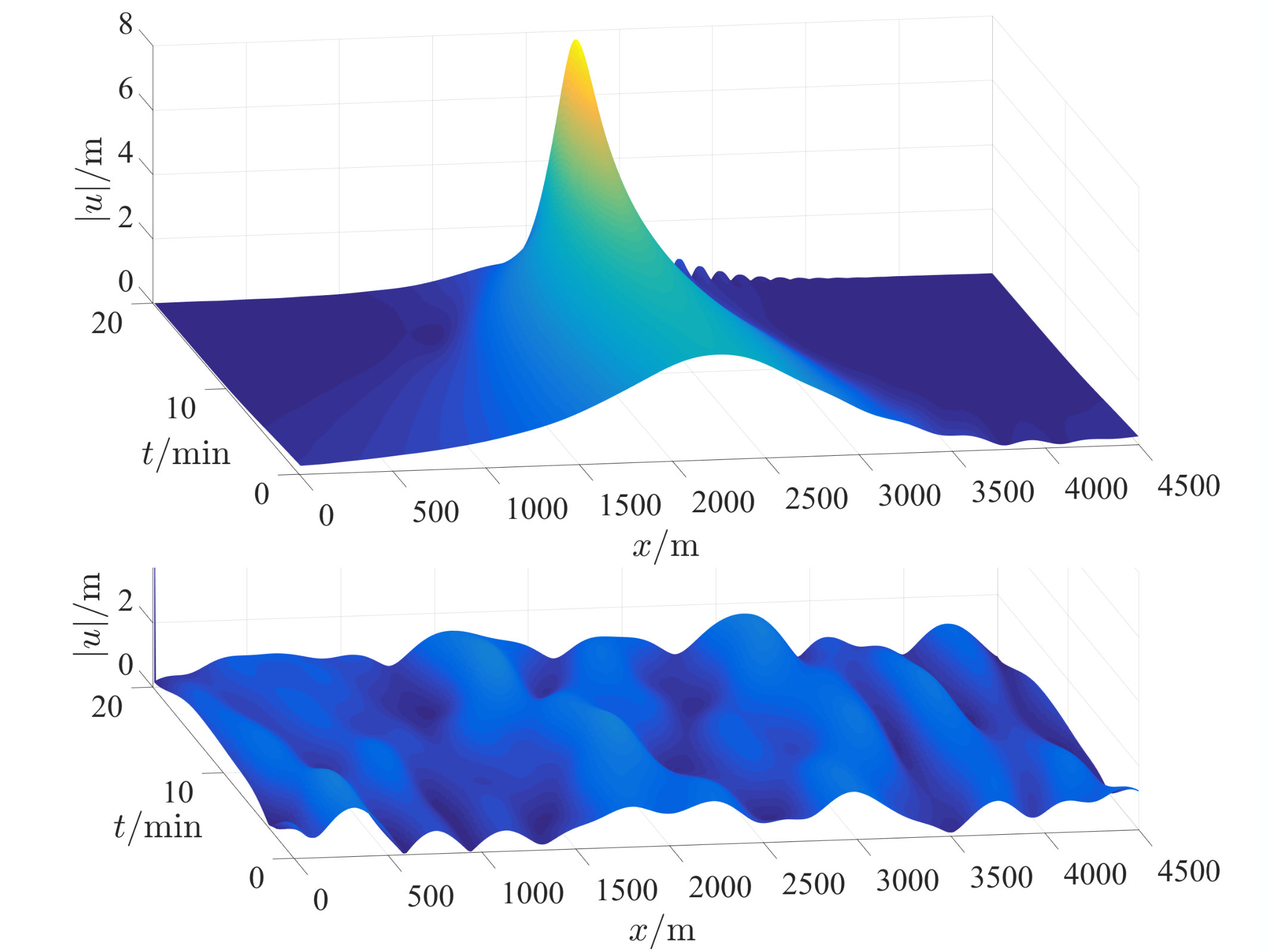 Figure 1
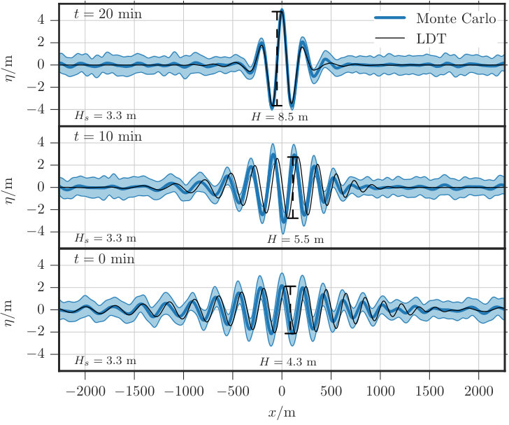 Figure 2
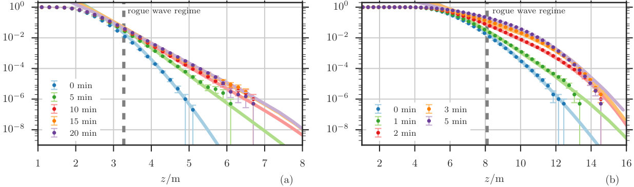 Figure 3
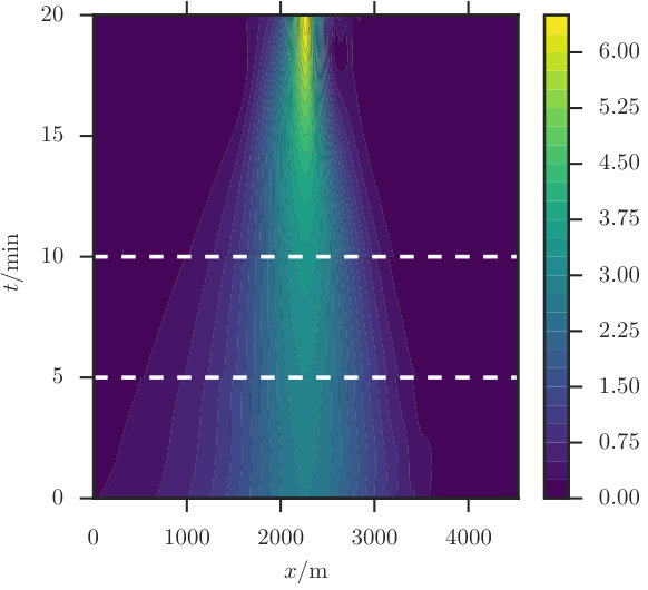 Figure 4
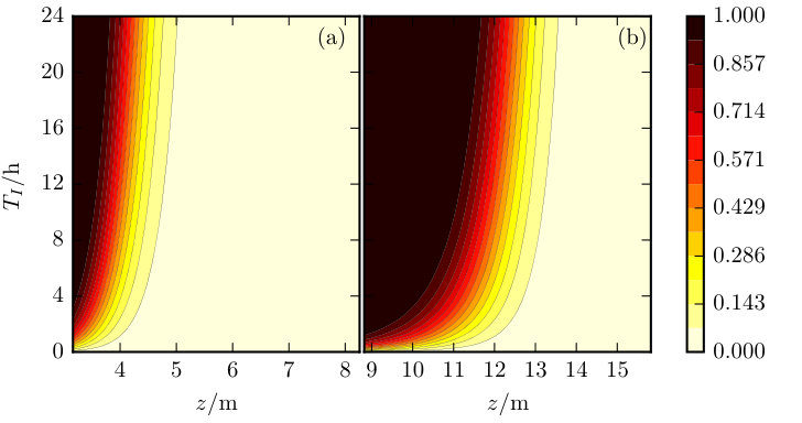 Figure 5
 Figure 6
Peer Reviews
No public reviews on file for this paper yet. If you reviewed it on a platform where reviews are public (OpenReview, ICLR, NeurIPS, ICML), you can paste yours below so the community can read it here.
Videos
No videos yet. Explain this paper in a talk, walkthrough, or lecture? Add one.
Rogue Waves and Large Deviations in Deep Sea
Giovanni Dematteis
Courant Institute, New York University, 251 Mercer Street, New York, NY 10012, USA
Dipartimento di Scienze Matematiche, Politecnico di Torino, Corso Duca degli Abruzzi 24, I-10129 Torino, Italy
Tobias Grafke
Mathematics Institute, University of Warwick, Coventry CV4 7AL, United Kingdom
Eric Vanden-Eijnden
Courant Institute, New York University, 251 Mercer Street, New York, NY 10012, USA
Abstract
The appearance of rogue waves in deep sea is investigated using the modified nonlinear Schrödinger (MNLS) equation in one spatial-dimension with random initial conditions that are assumed to be normally distributed, with a spectrum approximating realistic conditions of a uni-directional sea state. It is shown that one can use the incomplete information contained in this spectrum as prior and supplement this information with the MNLS dynamics to reliably estimate the probability distribution of the sea surface elevation far in the tail at later times. Our results indicate that rogue waves occur when the system hits unlikely pockets of wave configurations that trigger large disturbances of the surface height. The rogue wave precursors in these pockets are wave patterns of regular height but with a very specific shape that is identified explicitly, thereby allowing for early detection. The method proposed here combines Monte Carlo sampling with tools from large deviations theory that reduce the calculation of the most likely rogue wave precursors to an optimization problem that can be solved efficiently. This approach is transferable to other problems in which the system’s governing equations contain random initial conditions and/or parameters.
Rogue waves, long considered a figment of sailor’s imagination, are now recognized to be a real, and serious, threat for boats and naval structures muller2005rogue ; white1998chance . Oceanographers define them as deep water waves whose crest-to-trough height exceeds twice the significant wave height , which itself is four times the standard deviation of the ocean surface elevation. Rogue waves appear suddenly and unpredictably, and can lead to water walls with vertical size on the order of – m haver2004possible ; nikolkina2011rogue , with enormous destructive power. Although rare, they tend to occur more frequently than predicted by linear Gaussian theory onorato-residori-bortolozzo-etal:2013 ; nazarenko:2016 . While the mechanisms underlying their appearance remain under debate akhmediev2009extreme ; akhmediev2010editorial ; onorato2016origin , one plausible scenario has emerged over the years: it involves the phenomenon of modulational instability benjamin-feir:1967 ; zakharov:1968 , a nonlinear amplification mechanism by which many weakly interacting waves of regular size can create a much larger one. Such an instability arises in the context of the focusing nonlinear Schrödinger (NLS) equation zakharov:1968 ; kuznetsov:1977 ; peregrine:1983 ; akhmediev1987exact ; osborne2000nonlinear ; zakharov-ostrovsky:2009 ; onorato:2009 or its higher order variants dysthe:1979 ; stiassnie:1984 ; trulsen1996modified ; craig2010hamiltonian ; gramstad2011hamiltonian , which are known to be good models for the evolution of a unidirectional, narrow-banded surface wave field in a deep sea. Support for the description of rogue waves through such envelope equations recently came from experiments in water tanks onorato2004observation ; chabchoub2011rogue ; chabchoub2012super ; goullet2011numerical , where Dysthe’s MNLS equation in one spatial dimension dysthe:1979 ; stiassnie:1984 was shown to accurately describe the mechanism creating coherent structures which soak up energy from its surroundings. While these experiments and other theoretical works lo1985numerical ; cousins-sapsis:2015A give grounds for the use of MNLS to describe rogue waves, they have not addressed the question of their likelihood of appearance. Some progress in this direction has been recently made in cousins2016reduced , where a reduced model based on MNLS was used to estimate the probability of a given amplitude within a certain time, and thereby compute the tail of the surface height distribution. These calculations were done using an ansatz for the solutions of MNLS, effectively making the problem two-dimensional. The purpose of this paper is to remove this approximation, and study the problem in its full generality. Specifically, we consider the MNLS with random initial data drawn from a Gaussian distribution nazarenko2011wave . The spectrum of this field is chosen to have a width comparable to that of the JONSWAP spectrum hasselmann:1973 ; onorato:2001 obtained from observations in the North Sea. We calculate the probability of occurrence of a large amplitude solution of MNLS out of these random initial data, and thereby also estimate the tail of the surface height distribution. These calculations are performed within the framework of large deviations theory (LDT), which predicts the most likely way by which large disturbances arise and therefore also explains the mechanism of rogue wave creation. Our results are validated by comparison with brute-force Monte-Carlo simulations, which indicate that rogue waves in MNLS are indeed within the realm of LDT. Our approach therefore gives an efficient way to assess the probability of large waves and their mechanism of creation.
I Problem setup
Our starting point will be the MNLS equation for the evolution of the complex envelope of the sea surface in deep water dysthe:1979 , in terms of which the surface elevation reads \eta(t,x)=\Re\big{(}u(t,x)e^{i(k_{0}x-\omega_{0}t)}\big{)} (here denotes the carrier wave number, , and is the gravitational acceleration). Measuring and in units of and in we can write MNLS in non-dimensional form as
[TABLE]
where the bar denotes complex conjugation. We will consider Eq. 1 with random initial condition , constructed via their Fourier representation,
[TABLE]
where , are complex Gaussian variables with mean zero and covariance , . This guarantees that is a Gaussian field with mean zero and .To make contact with the observational data, the amplitude and the width in Eq. 2 are picked so that has the same height and area as the JONSWAP spectrum hasselmann:1973 ; onorato:2001 – see Supporting Information for details.
Because the initial data for Eq. 1 are random, so is the solution at time , and our aim is to compute
[TABLE]
where denotes probability over the initial data and is a scalar functional depending on at time . Even though our method is applicable to more general observables, here we will focus on
[TABLE]
II Large deviations theory approach
A brute force approach to calculate Eq. 3 is Monte-Carlo sampling: Generate random initial conditions by picking random ’s in Eq. 2, evolve each of these deterministically via Eq. 1 up to time to get , and count the proportion that fulfill . While this method is simple, and will be used below as benchmark, it looses efficiency when is large, which is precisely the regime of interest for the tails of the distribution of . In that regime, a more efficient approach is to rely on results from LDT which assert that Eq. 3 can be estimated by identifying the most likely initial condition that is consistent with . To see how this result comes about, recall that the probability density of is formally proportional to , where is given by
[TABLE]
To calculate Eq. 3 we should integrate this density over the set , which is hard to do in practice. Instead we can estimate the integral by Laplace’s method. As shown in Material and Methods, this is justified for large , when the probability of the set is dominated by a single that contributes most to the integral and can be identified via the constrained minimization problem
[TABLE]
which then yields the following LDT estimate for Eq. 3
[TABLE]
Here means that the ratio of the logarithms of both sides tends to 1 as . As discussed in Material and Methods, a multiplication prefactor can be added to (7) but it does not affect significantly the tail of on a logarithmic scale.
In practice, the constraint can be imposed by adding a Lagrange multiplier term to Eq. 6, and it is easier to use this multiplier as control parameter and simply see a posteriori what value of it implies. That is to say, perform for various values of the minimization
[TABLE]
over all of the form in Eq. 2 (no constraint), then observe that this implies the parametric representation
[TABLE]
where denotes the minimizer obtained in Eq. 8. It is easy to see from Eqs. 6 and 8 that is the Legendre transform of since:
[TABLE]
III Results
We considered two sets of parameters. In Set 1 we took and . Converting back into dimensional units using m consistent with the JONSWAP spectrum hasselmann:1973 ; onorato:2001 , this implies a significant wave height m classified as a rough sea WMO:2016 . It also yields a Benjamin-Feir index BFI, onorato:2001 ; janssen:2003 , meaning that the modulational instability of a typical initial condition is of medium intensity. In Set 2 we took and , for which m is that of a high sea and the BFI is 0.85, meaning that the modulational instability of a typical initial condition is stronger.
Fig. 1 (top) shows the time evolution of starting from an initial condition from Set 1 optimized so that m at min. For comparison, Fig. 1 (bottom) shows for a typical initial condition drawn from its Gaussian distribution. To illustrate what is special about the initial conditions identified by our optimization procedure, in Fig. 2 we show snapshots of the surface elevation at three different times, min (black lines), using the constraint that m at min. Additionally, we averaged all Monte-Carlo samples achieving m, translated to the origin. Snapshots of this mean configuration are shown in Fig. 2 (blue lines). They agree well with those of the optimized solution (black lines). The one standard deviation spread around the mean Monte-Carlo realization (light blue) is reasonably small, especially around the rogue wave at final time. This indicates that the event m is indeed realized with probability close to 1 by starting from the most likely initial condition consistent with this event, as predicted by LDT. The usefulness of LDT is confirmed in Figs. 3 (a,b) depicting the probabilities of for both Sets 1 and 2 calculated via LDT optimization (lines), compared to Monte-Carlo sampling (dots). As can be seen, the agreement is remarkable, especially in the tail corresponding to the rogue wave regime. As expected, the Monte-Carlo sampling becomes inaccurate in the tail, since there the probabilities are dominated by unlikely events. The LDT calculation, in contrast, remains efficient and accurate far in the tail.
The probabilities plotted in Fig. 3 (a,b) show several remarkable features. First, they indicate that, as gets larger, their tails fatten significantly. For example, in Set 1 , which is orders of magnitude larger than initially, . Secondly, the probabilities converge to a limiting density for large . This occurs after some decorrelation time min in Set 1 and min in Set 2. Similarly, the LDT results converge. In fact, this convergence can be observed at the level of the trajectories generated from the optimal . As Fig. 4 shows, reading these trajectories backward from , their end portions coincide, regardless on whether min, min, or min. The implications of these observations, in particular on the mechanism of creation of rogue waves and their probability of appearance within a time window, will be discussed in Interpretation below.
Before doing so, let us discuss the scalability of our results to larger domain sizes, referring the reader to the Supporting Information for more details. As shown above, the optimization procedure based on large deviation theory predicts that the most likely way a rogue wave will occur in the domain is via the apparition of a single large peak in . In the set-up considered before, this prediction is confirmed by the brute-force simulations using Monte-Carlo sampling. It is clear, however, that for increased domain size, e.g. by taking a domain size of with , it will become increasingly likely to observe multiple peaks, for the simple reason that large waves can occur independently at multiple sufficiently separated locations. In these large domains, the large deviation predictions remain valid if we look at the maximum of in observation windows that are not too large (that is, about the size of the domain considered above). However, they deteriorate if we consider this maximum in the entire domain of size , in the sense that the value predicted by large deviation theory matches that from Monte-Carlo sampling at values of that are pushed further away in the tails. This is an entropic effect, which is easy to correct for: events in different subwindows must be considered independent, and their probabilities superposed. That is, if we denote by
[TABLE]
it can be related to via
[TABLE]
This formula is derived in the Supporting Information and shown to accurately explain the numerical results. For efficiency is chosen to be the smallest domain size for which boundary effects can be neglected, in the sense that the shape of the optimal trajectories does no longer change if is increased further. In effect, this provides us with a method to scale up our results to arbitrary large observation windows.
IV Interpretation
The convergence of towards a limiting function has important consequences for the significance and interpretation of our method and its results. Notice first that this convergence can be explained if we assume that the probability distribution of the solutions to Eq. 1 with Gaussian initial data converges to an invariant measure. In this case, for large , the Monte-Carlo simulations will sample the value of on this invariant measure, and the optimization procedure based on LDT will do the same. The timescale over which convergence occurs depends on how far this invariant measure is from the initial Gaussian measure of . Interestingly the values we observe for are in rough agreement with the time scales predicted by the semi-classical limit of NLS that describes high-power pulse propagation bertola2013universality ; tikan2017universality . As recalled in the Supporting Information, this approach predicts that the timescale of apparition of a focusing solution starting from a large initial pulse of maximal amplitude and length-scale is , where is the nonlinear timescale for modulational instability and is the linear timescale associated to group dispersion. Setting (the size at the onset of rogue waves) and (the correlation length of the initial field) gives min for Set 1 and min for Set 2, consistent with the convergence times of . This observation has implications in terms of the mechanism of apparition of rogue waves, in particular their connection to the so-called Peregrine soliton, that has been invoked as prototype mechanism for rogue waves creation peregrine:1983 ; akhmediev2009waves ; shrira2010makes ; akhmediev2013recent ; onorato-residori-bortolozzo-etal:2013 ; toenger2015emergent , in particular for water waves chabchoub2011rogue ; chabchoub2012super ; chabchoub2016tracking , plasmas bailung2011observation and fiber optics kibler2010peregrine ; suret2016single ; tikan2017universality . This connection is discussed in the Supporting Information.
Our findings also indicate that, even though the assumption that is Gaussian is incorrect in the tail (that is, is not equal to the limiting in the tail), it contains the right seeds to estimate via if 111This convergence occurs on the timescale which is much smaller than the mixing time for the solutions of Eq. 1, i.e. the time it would take from a given initial condition, rather than an ensemble thereof, to sample the invariant measure.. Altogether this is consistent with the scenario put forward by Sapsis and collaborators in mohamad2016probabilistic ; farazmand-sapsis:2017 to explain how extreme events arise in intermittent dynamical systems and calculate their probability: they occur when the system hits small instability pockets which trigger a large transient excursion. In this scenario, as long as the initial probability distribution in these pockets is accurate, the dynamics will permit precise estimation of the distribution tail. In some sense, the distribution of the initial condition plays a role of the prior distribution in Bayesian inference222Note in particular that the Gaussian field in Eq. 2 is the random field that maximizes entropy given the constraint on its covariance ., and the posterior can be effectively sampled by adding the additional information from the dynamics over short periods of time during which instabilities can occur. In mohamad2016probabilistic , this picture was made predictive by using a two-dimensional ansatz for the initial condition to avoid having to perform sampling in high-dimension over the original . What our results show is that this approximation can be avoided altogether by using LDT to perform the calculations directly with the full Gaussian initial condition in Eq. 2.
Interestingly, we can use the results above to calculate the probability of occurrence of rogue waves in a given time window. More precisely, the probability that a rogue wave of amplitude larger than be observed in the domain during (i.e. that ) can be estimated in terms of and as
[TABLE]
where we used the fact that rogue waves can be considered independent on timescales larger than and assumed . The function is plotted in Fig. 5 as a function of and . For example for Set 1, Eq. 13 indicates a 50% chance to observe a rogue wave of height m (that is, about 8 m from crest-to-trough) after 11 hours (using min and ); if we wait 30 hours, the chance goes up to 85%. Similarly, for Set 2 the chance to observe a wave of 11 m height is about 50% after 3 hours and about 85% after 8 hours ( min and ).
V Concluding remarks
We have shown how an optimization problem building on LDT can be used to predict the pathway and likelihood of appearance of rogue waves in the solutions of MNLS fed by random initial data consistent with observations. This setup guarantees accuracy of the core of the initial distribution, which in turn permits the precise estimation of its tail via the dynamics. Our results give quantitative estimate for the probabilities of observing high amplitude waves within a given time window. These results also show that rogue waves have very specific precursors, a feature that was already noted in farazmand2017reduced in the context of a reduced model and could potentially be used for their early detection.
VI Materials and Methods
VI.1 Laplace method and large deviations
For the reader’s convenience, here we recall some standard large deviations results that rely on the evaluation of Gaussian integrals by Laplace’s method and are at the core of the method we propose. It is convenient to rephrase the problem abstractly and consider the estimation of
[TABLE]
where are Gaussian random variables with mean zero and covariance Id, and is some real valued function – as long as we truncate the sum in Eq. 2 to a finite number of modes, , the problem treated in this paper can be cast in this way, with playing the role of and that of . The probability in Eq. 14 is given by
[TABLE]
where . The interesting case is when this set does not contain the origin, , which we will assume is true when . We also make two additional assumptions:
The point on the boundary that is closest to the origin is isolated: Denoting this point as
[TABLE]
we assume that
[TABLE] 2. 2.
The connected piece of that contains is smooth with a curvature that is bounded by a constant independent of .
The point satisfies the Euler-Lagrange equation for Eq. 16, with the constraint incorporated via a Lagrange multiplier term:
[TABLE]
for some Lagrange multiplier . This implies that
[TABLE]
where denotes the inward pointing unit vector normal to at . If we move inside the set from in the direction of , the norm increases under the assumptions in Eq. 17. Indeed, setting with , we have
[TABLE]
where we used Eq. 19. In fact, if we were to perform the integral in that direction, the natural variable of integration would be to rescale . In particular, if we were to replace by the half space , it would be easy to estimate the integral in Eq. 15 by introducing a local coordinate system around , whose first coordinate is in the direction of . Indeed this would give:
[TABLE]
The last approximation goes beyond a large deviations estimate (i.e. it includes the prefactor), and it implies
[TABLE]
This log-asymptotic estimate is often written as
[TABLE]
Interestingly, while the asymptotic estimate in Eq. 21 does not necessarily apply to the original integral in Eq. 15 (that is, the prefactor may take different forms depending on the shape of near ), the rougher log-asymptotic estimate in Eq. 23 does as long as the the boundary is smooth, with a curvature that is bounded by a constant independent of . This is because because the contribution (positive or negative) to the integral over the region between and is subdominant in that case, in the sense that the log of its amplitude is dominated by . This is the essence of the large deviations result that we apply in this paper.
VI.2 Numerical aspects
To perform the calculations, we solved Eq. 1 with and periodic boundary conditions, and checked that this domain is large enough to make the effect of these boundary conditions negligible (see Supporting Information). The spatial domain was discretized using equidistant gridpoints, which is enough to resolve the solution of Eq. 1. To evolve the field in time we used a pseudo-spectral second order exponential time-differencing (ETD2RK) method cox:2002 ; kassam:2005 .
When performing the Monte-Carlo simulations, we used realizations of the random initial data constructed by truncating the sum in Eq. 2 over the modes with , i.e : these modes carry most of the variance, and we checked that adding more modes to the initial condition did not affect the results in any significant way (see Supporting Information).
VI.3 Optimization procedure
As explained above, the large deviation rate function in Eq. 6 can be evaluated by solving the dual optimization problem in Eq. 8, which we rewrite as , where we defined the cost function
[TABLE]
We performed this minimization using steepest descent with adaptive step (line-search) and preconditioning of the gradient borzi2011computational . This involves evaluating the (functional) gradient of with respect to . Using the chain rule, this gradient can be expressed as (using compact vectorial notation)
[TABLE]
where is the Jacobian of the transformation . Collecting all terms on the right-hand-side of the MNLS Eq. 1 into , this equation can be written as
[TABLE]
and it is easy to see that in this notation satisfies
[TABLE]
Consistent with what was done in the Monte-Carlo sampling, to get the results presented above we truncated the initial data over modes using the representation
[TABLE]
This means that minimization of Eq. 24 was performed in the dimensional space spanned by the modes , accounting for invariance by an overall phase shift – to check convergence we also repeated this calculation using larger values of and found no noticeable difference in the results (see Supporting Information).
In practice, the evaluation of the gradient in Eq. 25 was performed by integrating both and up to time . Eq. 27 was integrated using the same pseudo-spectral method as for Eq. 1 on the same grid. To perform the steepest descent step, we then preconditioned the gradient through scalar multiplication by the step-independent, diagonal metric with the components of the spectrum as diagonal elements.
Acknowledgment
We thank W. Craig and M. Onorato for helpful discussions, and O. Bühler, M. Mohamad, and T. Sapsis for interesting comments. We also thank the anonymous reviewer for drawing our attention to the semi-classical theory for the Nonlinear Schrödinger Equation. GD is supported by the joint Math PhD program of Politecnico and Università di Torino. EVE is supported in part by the Materials Research Science and Engineering Center (MRSEC) program of the National Science Foundation (NSF) under award number DMR-1420073 and by NSF under award number DMS-1522767.
The reference list from the paper itself. Each links out to its DOI / PubMed record.
- 1(1) Müller P, Garrett C, Osborne A (2005) Rogue waves. Oceanography 18(3):66.
- 2(2) White BS, Fornberg B (1998) On the chance of freak waves at sea. J. Fluid Mech. 355:113–138.
- 3(3) Haver S (2004) A possible freak wave event measured at the draupner jacket january 1 1995. Rogue waves 2004 pp. 1–8.
- 4(4) Nikolkina I, Didenkulova I (2011) Rogue waves in 2006–2010. Nat. Hazards Earth Syst. Sci. 11(11):2913–2924.
- 5(5) Onorato M, Residori S, Bortolozzo U, Montina A, Arecchi F (2013) Rogue waves and their generating mechanisms in different physical contexts. Phys. Rep. 528(2):47–89.
- 6(6) Nazarenko S, Lukaschuk S (2016) Wave turbulence on water surface. Annu. Rev. Condens. Matter Phys. 7:61–88.
- 7(7) Akhmediev N, Soto-Crespo JM, Ankiewicz A (2009) Extreme waves that appear from nowhere: on the nature of rogue waves. Physics Letters A 373(25):2137–2145.
- 8(8) Akhmediev N, Pelinovsky E (2010) Editorial–introductory remarks on “discussion & debate: Rogue waves–towards a unifying concept?”. Eur. Phys. J. Special Topics 185(1):1–4.