An acoustic glottal source for vocal tract physical models
Antti Hannukainen, Juha Kuortti, Jarmo Malinen, Antti Ojalammi

TL;DR
This paper introduces an acoustic glottal source and signal processing algorithms for measuring and reconstructing vocal tract physical models, validated on a male vowel model, enhancing acoustic measurement techniques.
Contribution
It presents a novel acoustic source and software for physical vocal tract models, enabling improved amplitude response and waveform reconstruction capabilities.
Findings
Validated on a male vowel model
Accurate amplitude frequency response measurements
Effective waveform reconstruction at the mouth
Abstract
A sound source was proposed for acoustic measurements of physical models of the human vocal tract. The physical models are produced by Fast Prototyping, based on Magnetic Resonance Imaging during prolonged vowel production. The sound source, accompanied by custom signal processing algorithms, is used for two kinds of measurements: (i) amplitude frequency response and resonant frequency measurements of physical models, and (ii) signal reconstructions at the source output according to a target waveform with measurements at the mouth position of the physical model. The proposed source and the software are validated by measurements on a physical model of the vocal tract corresponding to vowel [a] of a male speaker.
Click any figure to enlarge with its caption.
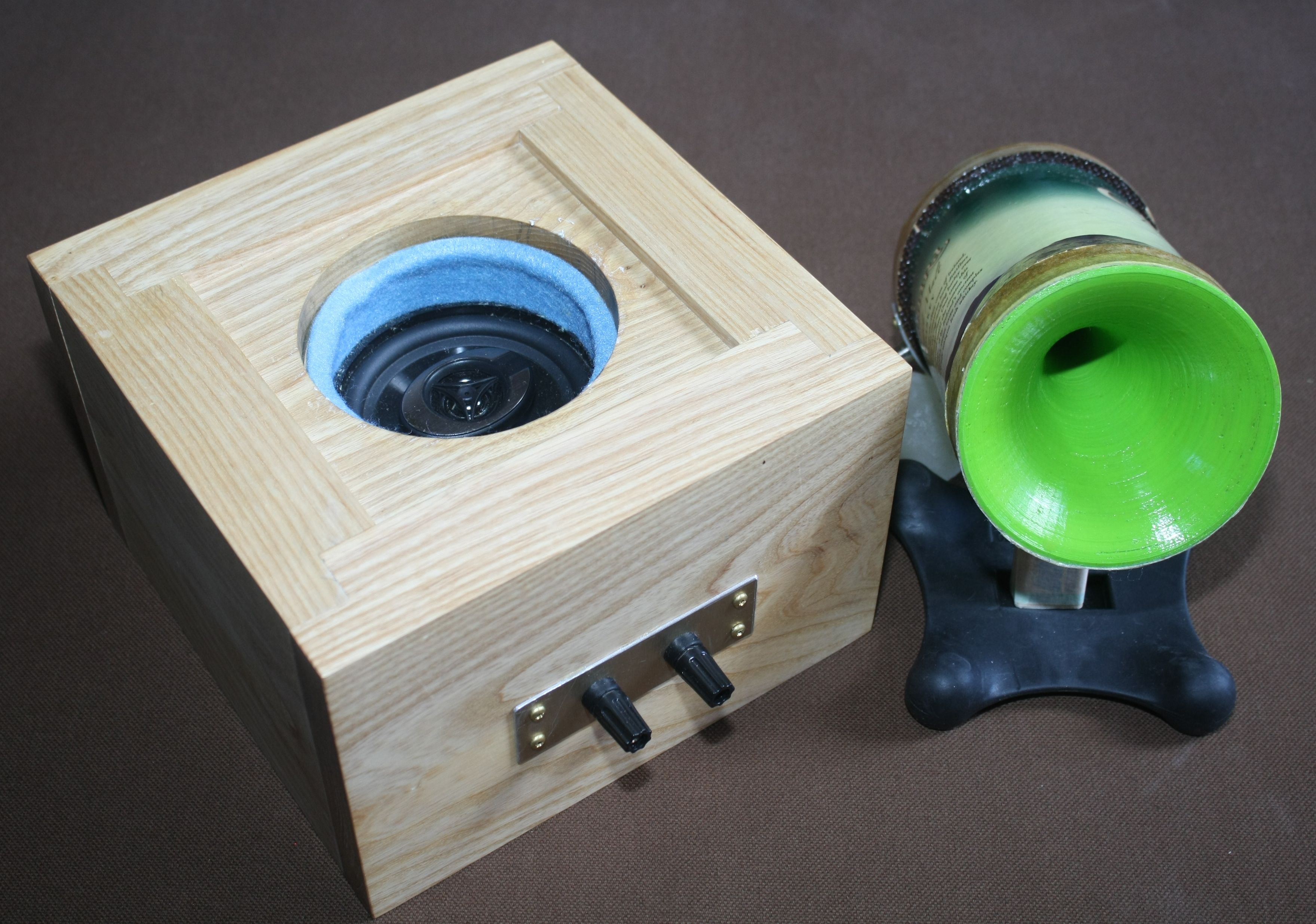 Figure 1
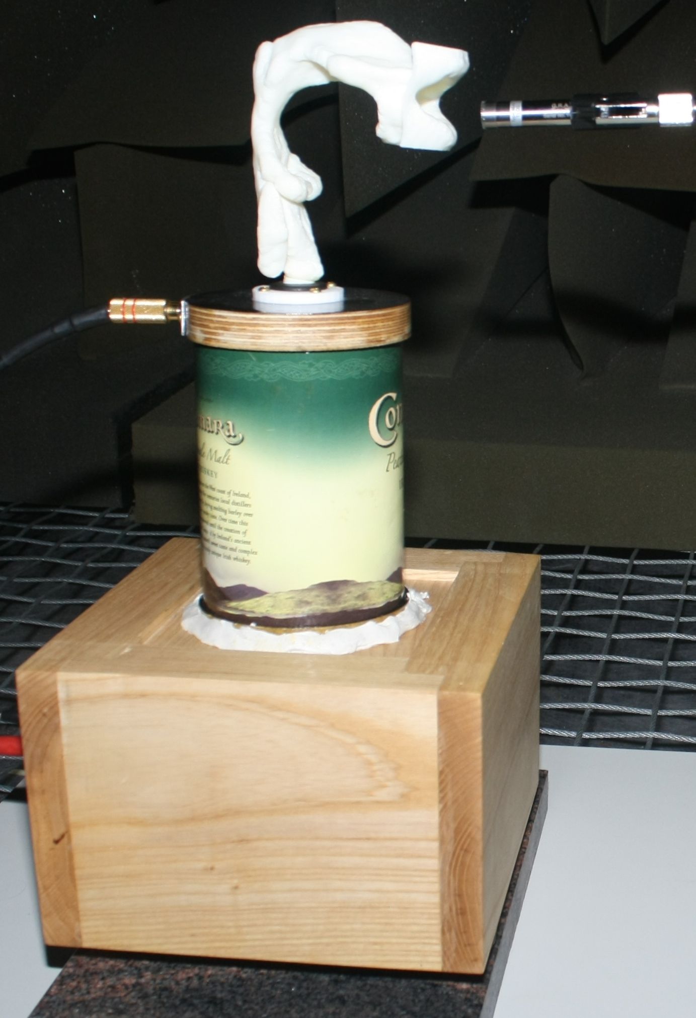 Figure 2
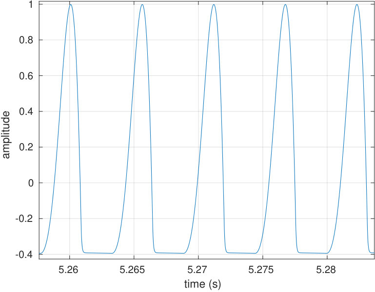 Figure 3
 Figure 4
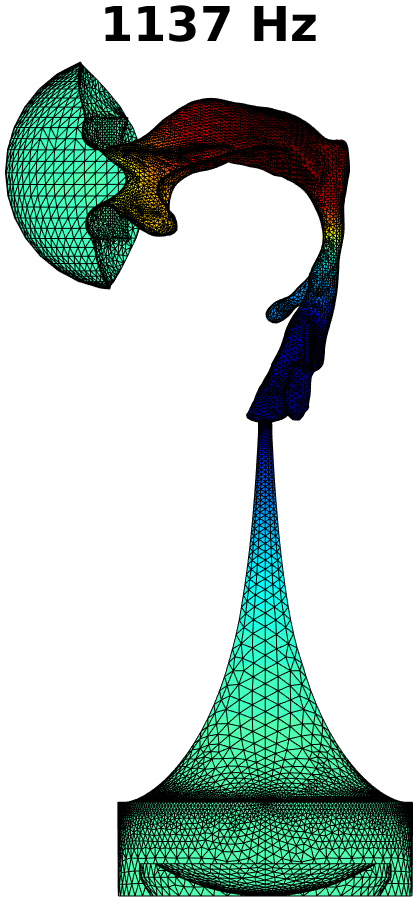 Figure 5
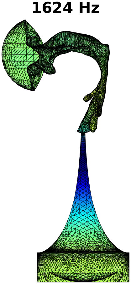 Figure 6
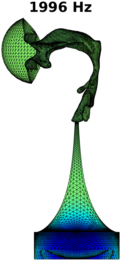 Figure 7
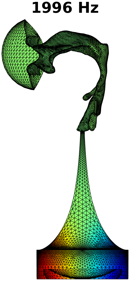 Figure 8
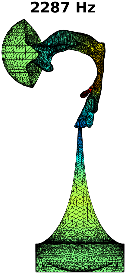 Figure 9
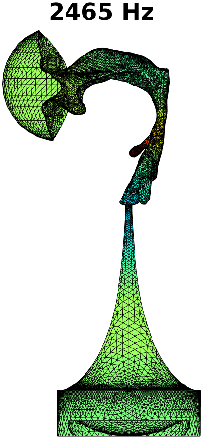 Figure 10
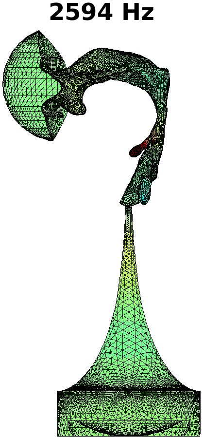 Figure 11
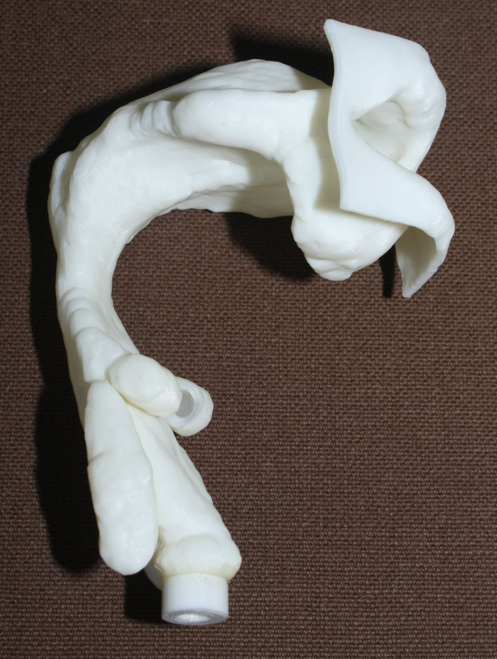 Figure 12
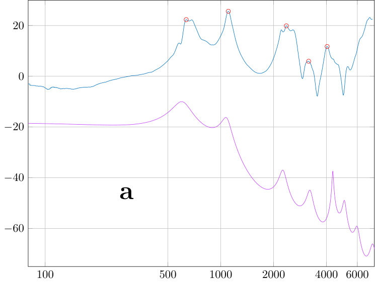 Figure 13
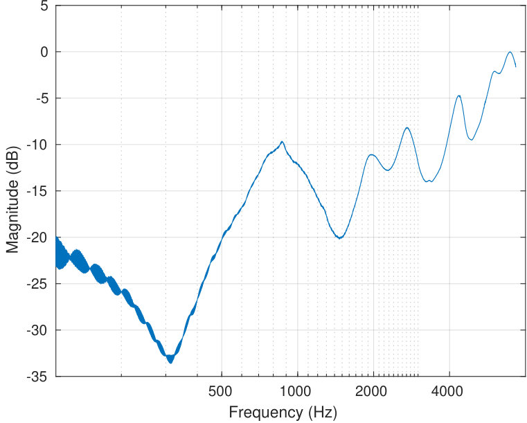 Figure 14
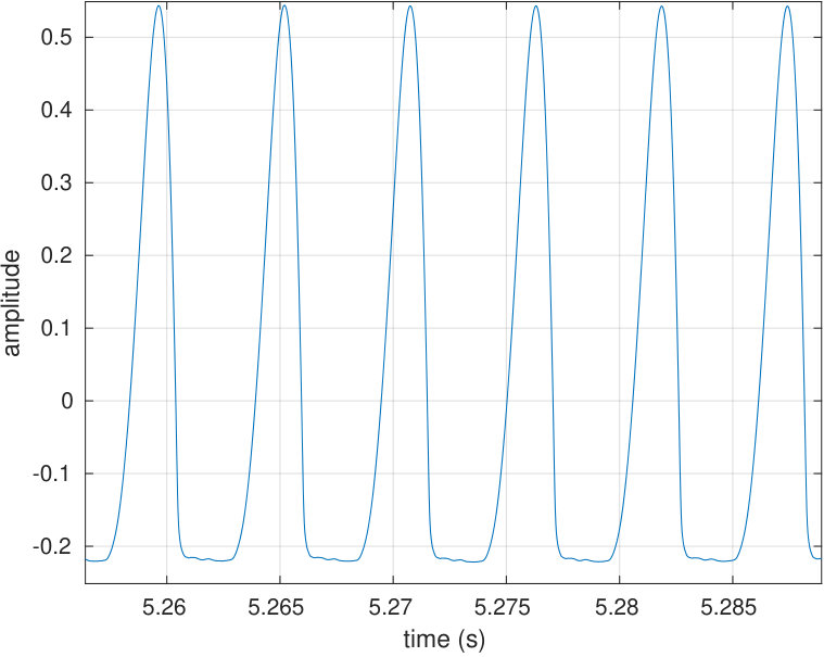 Figure 15
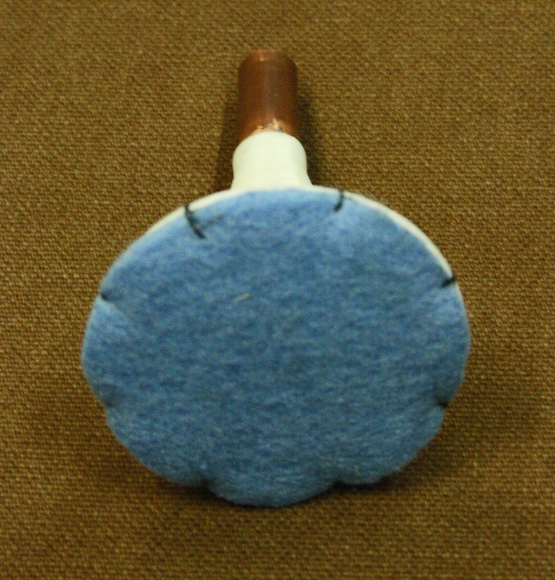 Figure 16
 Figure 17
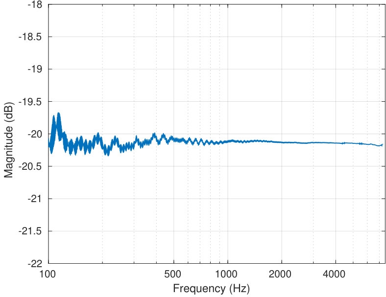 Figure 18
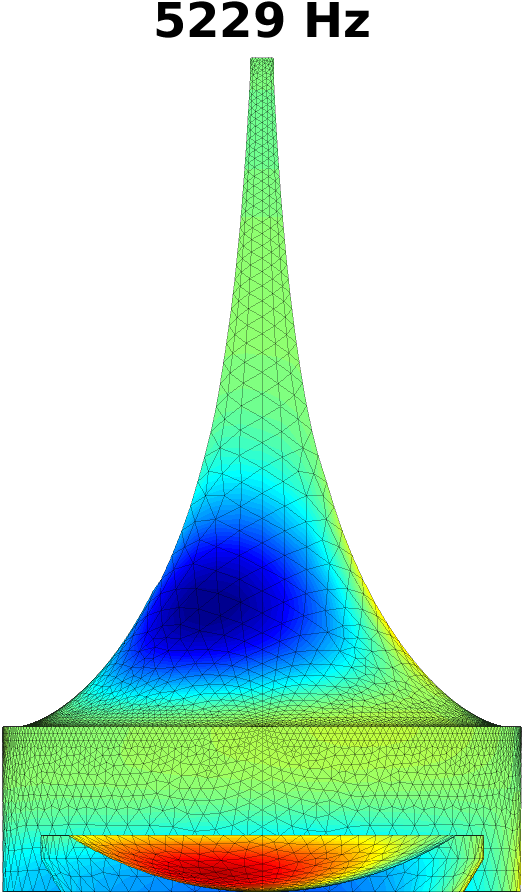 Figure 19
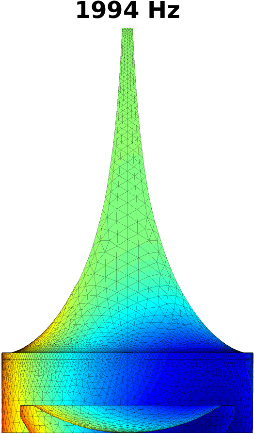 Figure 20
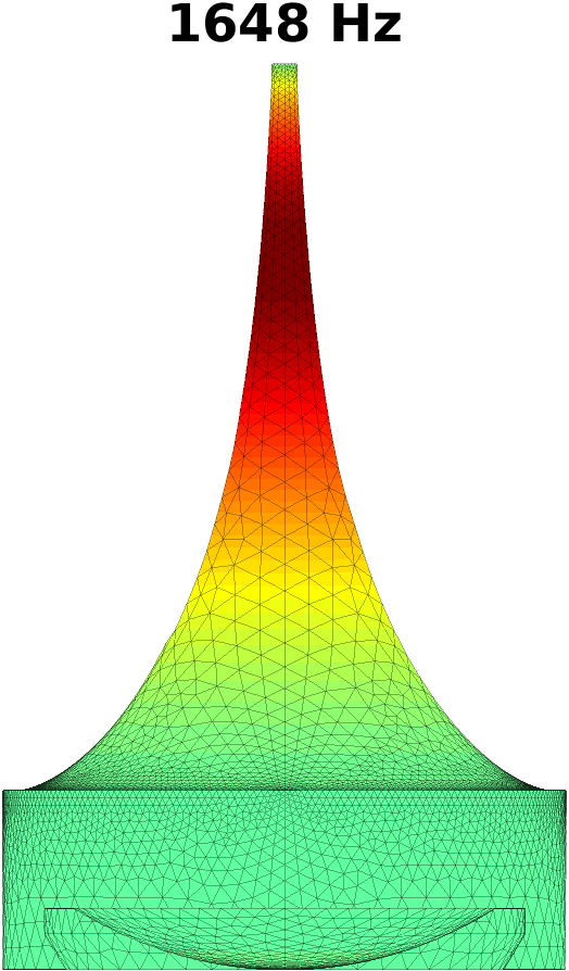 Figure 21
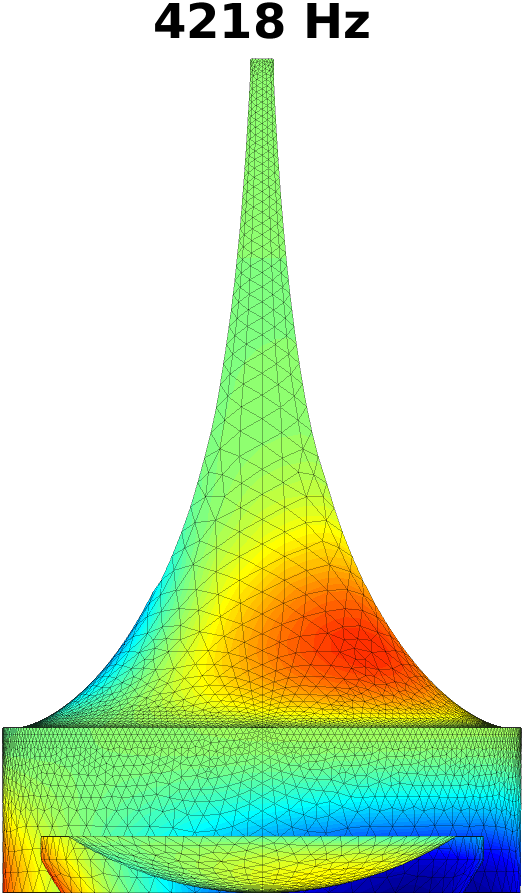 Figure 22
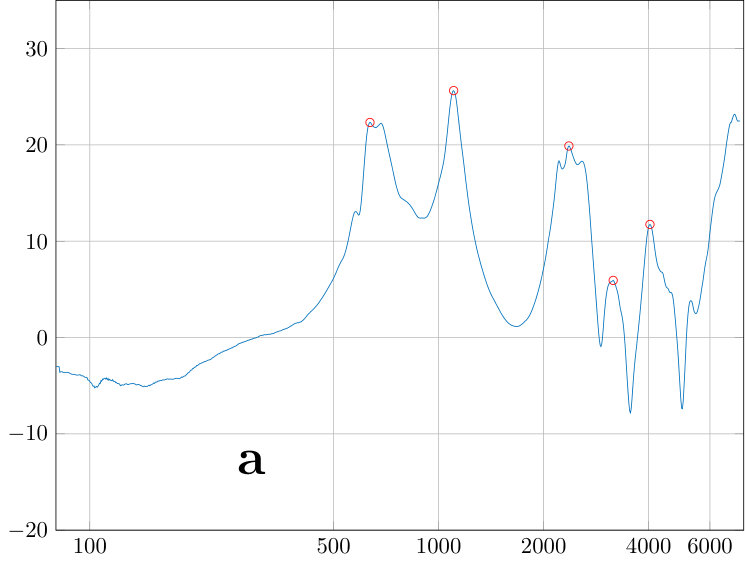 Figure 23
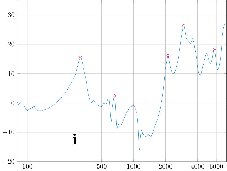 Figure 24
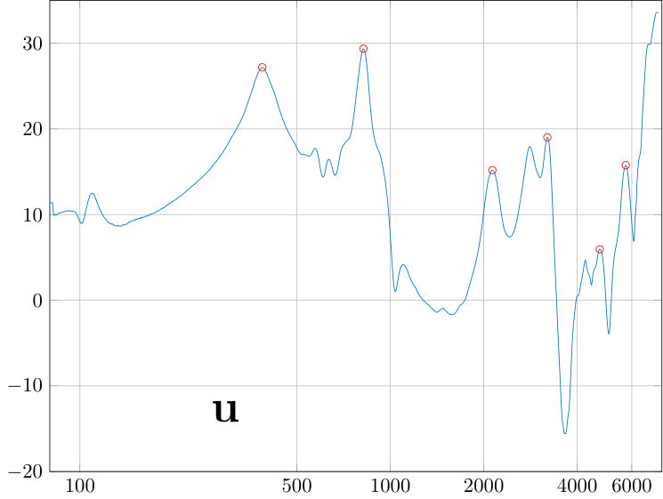 Figure 25
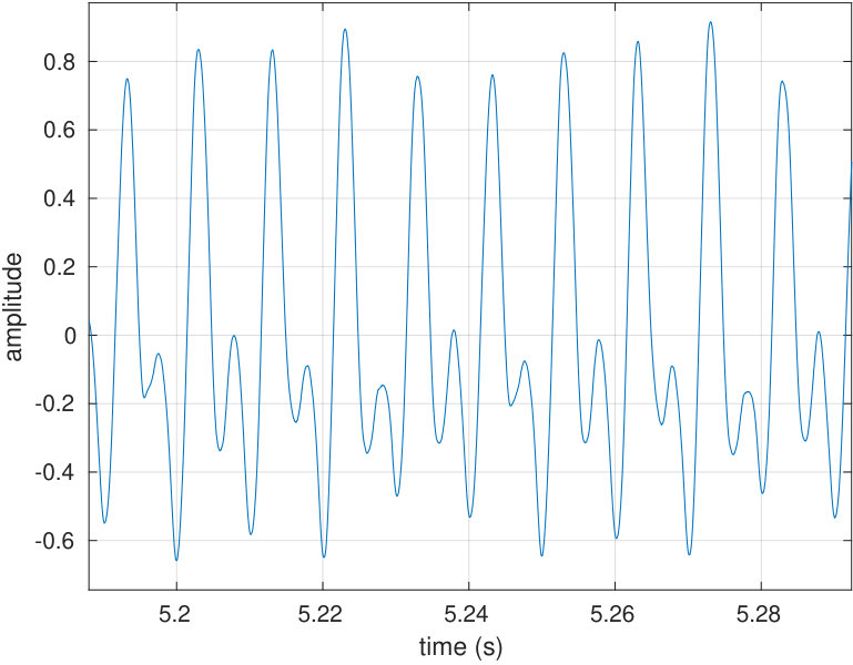 Figure 26
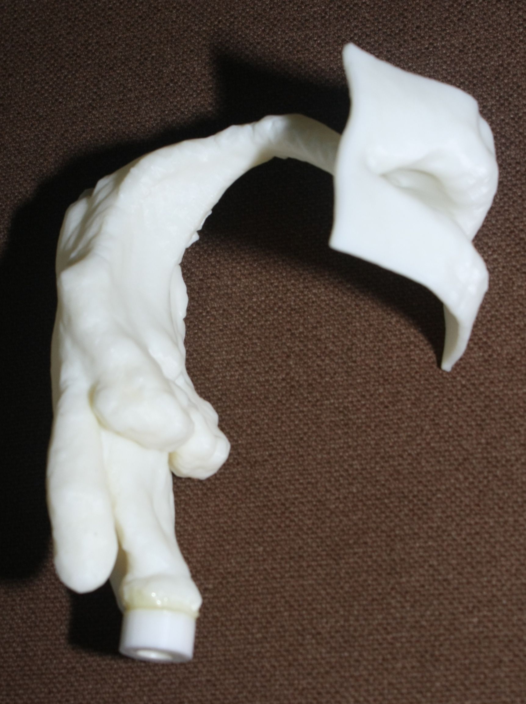 Figure 27
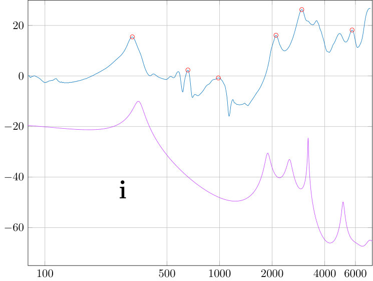 Figure 28
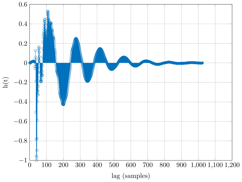 Figure 29
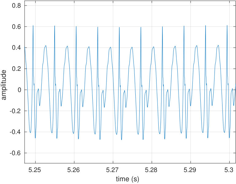 Figure 30
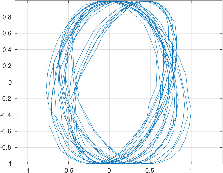 Figure 31
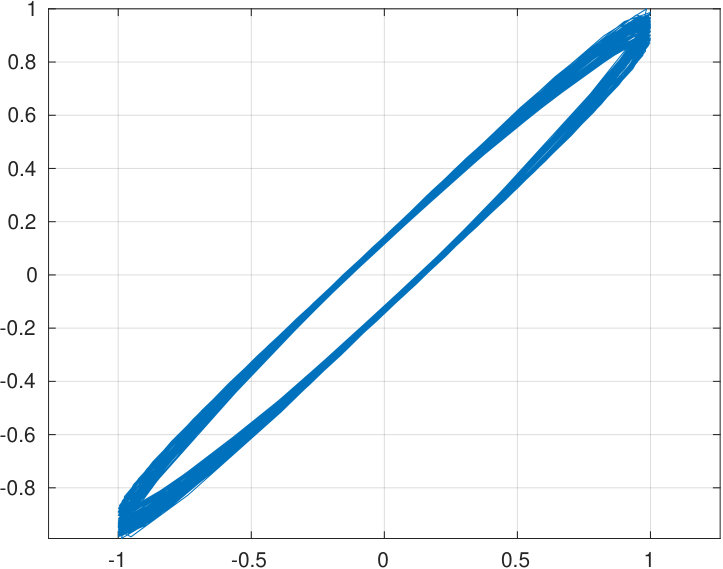 Figure 32
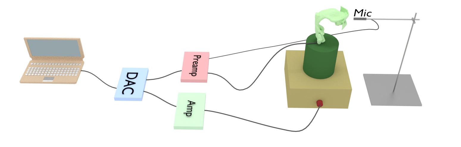 Figure 33
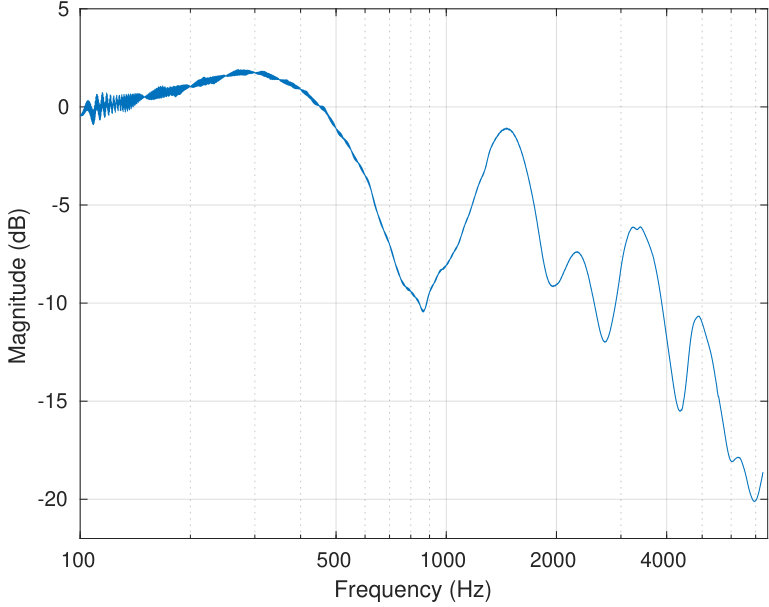 Figure 34
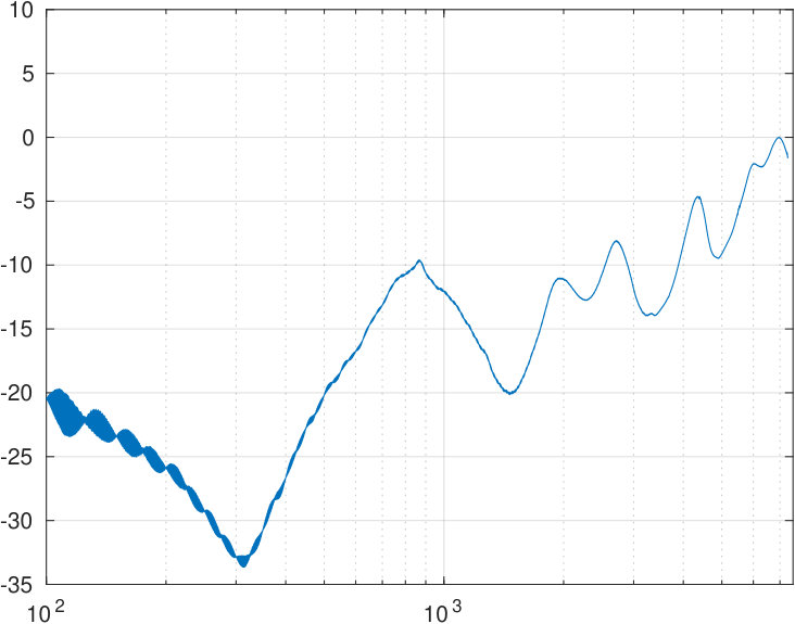 Figure 35
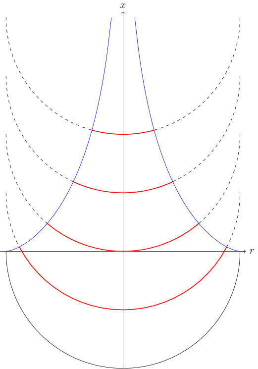 Figure 36
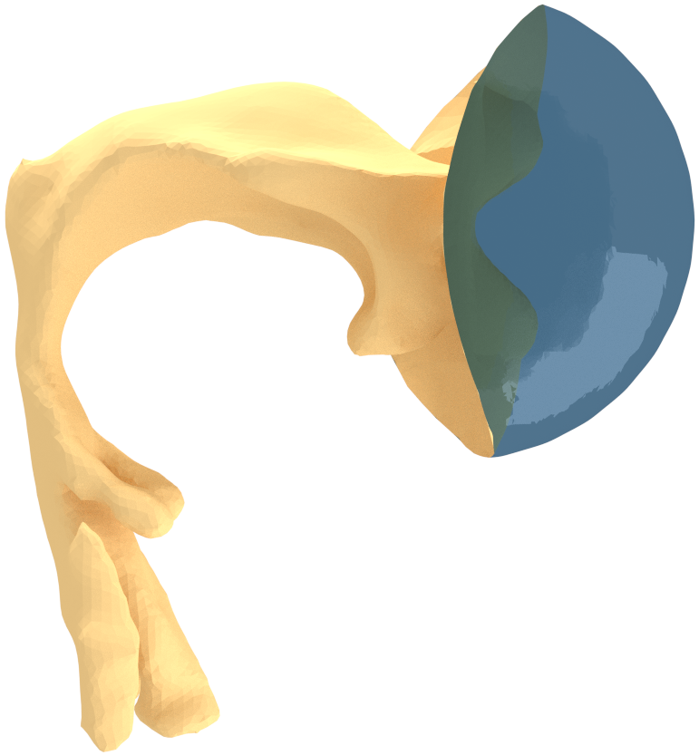 Figure 37
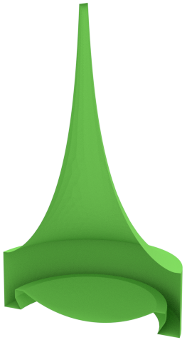 Figure 38
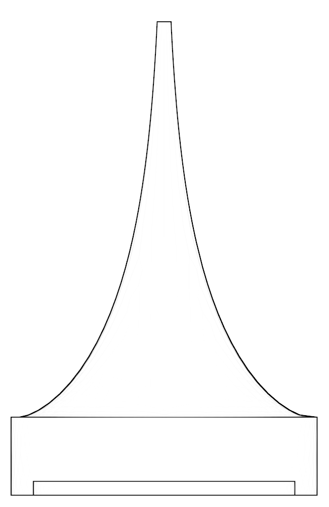 Figure 39
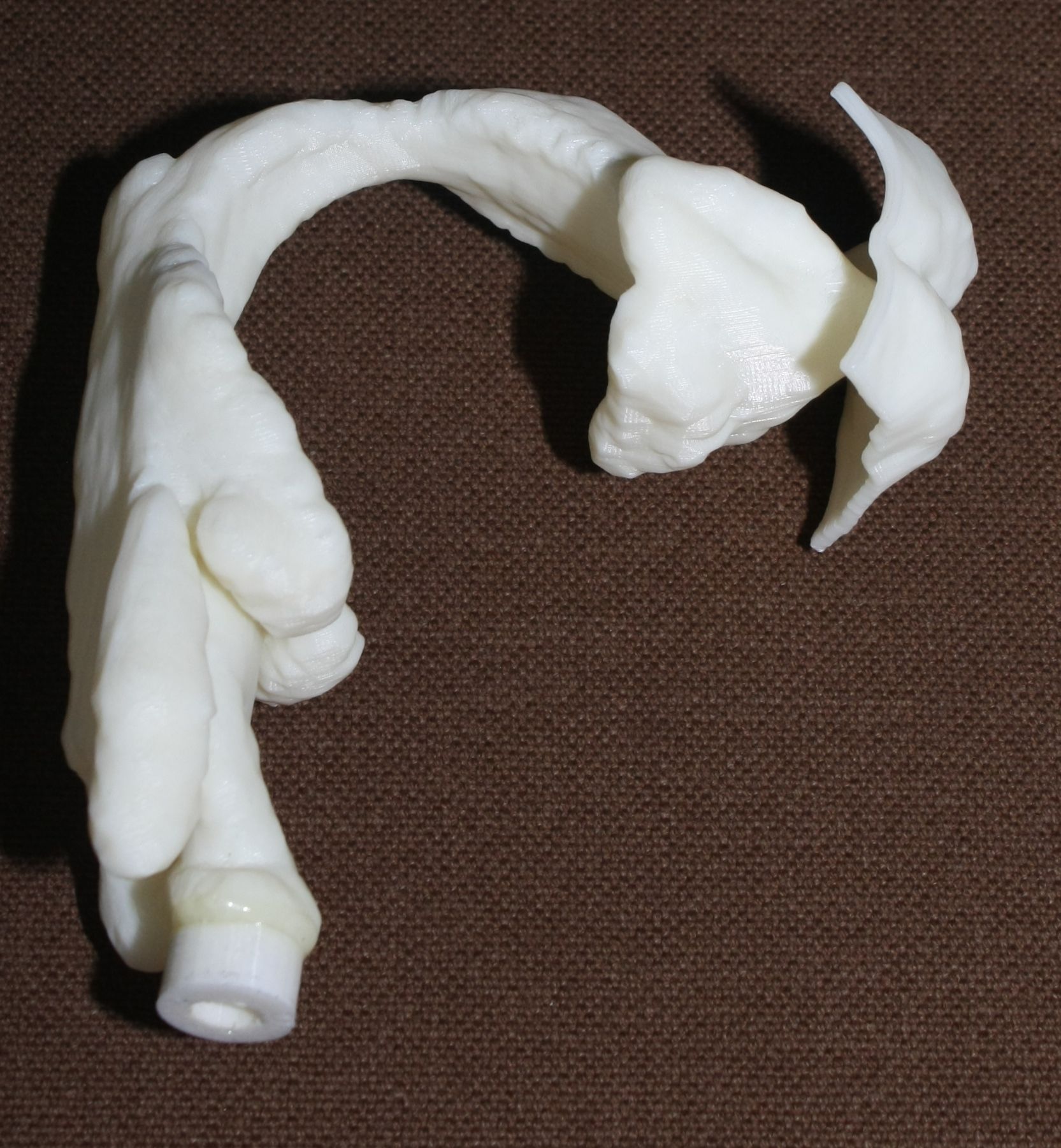 Figure 40
Peer Reviews
No public reviews on file for this paper yet. If you reviewed it on a platform where reviews are public (OpenReview, ICLR, NeurIPS, ICML), you can paste yours below so the community can read it here.
Videos
No videos yet. Explain this paper in a talk, walkthrough, or lecture? Add one.
An acoustic glottal source
for vocal tract physical models
Antti Hannukainen
Juha Kuortti
Jarmo Malinen
Antti Ojalammi
Dept. Mathematics and Systems Analysis, Aalto University, Finland
Dept. Signal Processing and Acoustics, Aalto University, Finland
Abstract
A sound source was proposed for acoustic measurements of physical models of the human vocal tract. The physical models are produced by Fast Prototyping, based on Magnetic Resonance Imaging during prolonged vowel production. The sound source, accompanied by custom signal processing algorithms, is used for two kinds of measurements: (i) amplitude frequency response and resonant frequency measurements of physical models, and (ii) signal reconstructions at the source output according to a target waveform with measurements at the mouth position of the physical model. The proposed source and the software are validated by measurements on a physical model of the vocal tract corresponding to vowel [] of a male speaker.
keywords:
Vowels , physical models , glottal source , measurements.
††journal: Measurement
1 Introduction
Acquiring comprehensive data from human speech is a challenging task that, however, is crucial for understanding and modelling speech production as well as developing speech signal processing algorithms. The possible approaches can be divided into direct and indirect methods. Direct methods concern measurements carried out on test subjects either by audio recordings, acquisition of pressure, flow velocity, or even electrical signals (such as takes place in electroglottography), or using different methods of medical imaging during speech. Indirect methods concern simulations using computational models (such as described in [1] and the references therein) or measurements from physical models111Physical models are understood as artefacts or replicas of parts of the speech anatomy in the context of this article.. Typically, computational and physical models are created and evaluated based on data that has first been acquired by direct methods. The main advantage of indirect methods is the absence of the human component that leads to experimental restrictions and unwanted variation in data quality.
The purpose of this article is to describe an experimental arrangement, its validation, and some experiments on one type of physical model for vowel production: acoustic resonators corresponding to vocal tract (VT) configurations during prolonged vowel utterance. The anatomic geometry for such resonators has been imaged by Magnetic Resonance Imaging (MRI) with simultaneous speech recordings as described in [2, 3]. The MRI voxel data has been processed to surface models as explained in [4] and then printed in ABS plastic by Rapid Prototyping as explained below in Section 2.5. In itself, the idea of using 3D printed VT models in speech research is by no means new: see, e.g., [5, 6, 7].
Just creating physical models of the VT is not enough for model experiments: also a suitable acoustic signal source is required with custom instrumentation and software associated to it. As these experiments involve a niche area in speech research, directly applicable commercial solutions do not exists and constructing a custom measurement suite looks an attractive option. Thus, we propose an acoustic glottal source design shown in Fig. 1 that resembles the loudspeaker-horn constructions shown in [5, Fig. 1], [6, Fig. 3], [8, Fig. 2a] .
All such source/horn constructions can be regarded as variants of compression drivers used as high impedance sources for horn loudspeakers. Unfortunately, most commercially available compression drivers are designed for frequencies over whereas a construction based on a loudspeaker unit can easily be scaled down to lower frequencies required in speech research. We point out that high quality acoustic measurements on VT physical models can be carried out using a measurement arrangement not based an impedance matching horn or a compression driver of some other kind; see [7, Fig. 3] where the sound pressure is fed into the model through the mouth opening, and the measurements are carried out using a microphone at the vocal folds position. However, excitation from the glottal position is desirable because the face and the exterior space acoustics are issues as well.
The general principle of operation of the acoustic glottal source is fairly simple. The source consists of a loudspeaker unit and an impedance matching horn as shown disassembled in Fig. 1 (middle panel). The purpose of the horn is to concentrate the acoustic power from the low-impedance loudspeaker to an opening of diameter , the high-impedance output of the source. There is, however, a number of conflicting design objectives that need be taken into account in a satisfactory way. For example, the instrument should not be impractically large, and it should be usable for acoustic measurements of physical models of human VTs in the frequency range of interest, specified as in this article. To achieve these goals in a meaningful manner, we use a design methodology involving (i) heuristic reasoning based on mathematical acoustics, together with (ii) numerical acoustics modelling of the main components and their interactions. Numerical modelling of all details is not necessary for a successful outcome. Optimising the source performance using only the method of trial and error and extensive laboratory measurements would be overly time consuming as well.
The design and construction process was incremental, and it consisted of the following steps that were repeated when necessary:
- (i)
Choice of the acoustic design and the main components, based on general principles of acoustics, horn design, and feasibility, 2. (ii)
Finite element (FEM) based modelling of the horn acoustics to check overall validity of the approach, to detect and then correct the expected problems in construction, 3. (iii)
the construction of the horn and the loudspeaker assembly together with the required instrumentation, 4. (iv)
a cycle of measurements and modifications, such as placement of acoustically soft material and silicone sealings in various parts based on, e.g., the FEM modelling, 5. (v)
development of MATLAB software for producing properly weighted measurement signals for sweep experiments that compensate most of the remaining nonidealities, and 6. (vi)
development of MATLAB software for reproducing the Liljencrants–Fant (LF) glottal waveform excitation at the glottal position of the physical models.
Finally, the source is used for measuring the frequency responses of physical models of VT during the utterance of Finnish vowels [, i, u], obtained from a 26-year-old male (in fact, one of the authors of this article). The measured amplitude frequency responses are compared with the spectral envelope data from vowel samples shown in Fig. 9, recorded in anechoic chamber from the same test subject. In addition to these responses, vowel signal is produced by acoustically exciting the physical models by a glottal pulse waveform of LF type, reconstructed at the output of the source. The produced signals for vowels [, i, u] have good audible resolution from each other, yet they have the distinct ``robotic'' sound quality that is typical of most synthetically produced speech.
Resonant frequencies extracted from the measured frequency responses are used for development and validation of acoustic and phonation models such as the one introduced in [1]. The synthetic vowel signals are intended for benchmarking Glottal Inverse Filtering (GIF) algorithms as was done in [9, 10]. Large amounts of measurement data are required for these applications which imposes requirements to the measurement arrangement.
So as to physical dimension of the measured signals, this article restricts to sound pressure measurements using microphones. If acoustic impedances are to be measured instead, some form of acoustic (perturbation) velocity measurement need be carried out. The velocity measurement can be carried out, e.g., by hot wire anemometers [11], impedance heads consisting of several microphones [12], or even by a single microphone using a resistive calibration load coupled to a high impedance source [13]; see [14, Table 1] for various approaches. In general, carrying out velocity measurements is much more difficult and expensive that measuring just sound pressure. Determining pressure-to-pressure -responses of VT physical models is, however, sufficient for the purposes of this article since (i) resonant frequencies can be determined from pressures, and (ii) the GIF algorithm can be configured to run on pressure data.
2 Background
We review relevant aspects from mathematical acoustics, horn design, signal processing, and MRI data acquisition.
2.1 Acoustic equations for horns
Acoustic horns are impedance matching devices that can be described as surfaces of revolution in a three-dimensional space. Thus, they are defined by strictly nonnegative continuous functions where , being the length of the horn, and denoting the radius of horn at . The end () is the input end (respectively, the output end) of the horn. It is typical, though not necessary, that the function is either increasing or decreasing.
There exists a wide literature on the design of acoustic (tractrix) horns for loudspeakers; see, e.g., [15, 16, 17, 18]. As a general rule, the matching impedance at an end of the horn is inversely proportional to the opening area. For uniform diameter waveguides, the matching impedance coincides with the characteristic impedance given by where is the intersectional area. The constant denotes the speed of sound and is the density of the medium.
To describe the acoustics of an air column in a cavity such as a horn, we use two (partial) differential equations. The three dimensional acoustics is described by the lossless Helmholtz equation in terms of the velocity potential
[TABLE]
where the acoustic domain is denoted by with boundary . A part of the boundary, denoted by , is singled out as an interface to the exterior space. In horn designs of Section 3.1, the interface is the opening at the narrow output end of the horn. In Section 4, the symbol denotes a spherical interface around the mouth opening. For now, we use the Dirichlet boundary condition on
[TABLE]
Eqs. (1)– (2) have a countably infinite number of solutions for , and each of the solutions is associated to a Helmholtz resonant frequency of by .
In addition to acoustic resonances, the acoustic transmission impedance of the source is important. Because it is more practical to deal with scalar impedances, we use the lossless Webster's resonance model for defining it, again in terms of Webster's velocity potential. It is given for any by
[TABLE]
where is the intersectional area of the horn, is the density of air, and is the termination resistance at the output end 222Because the external termination resistance is the only loss term in Eq. (3), we call the model lossless.. Again, the frequencies and Laplace transform domain variables are related by . The function is the Laplace transform of the (perturbation) volume velocity used to drive the horn, and the output is similarly given as the Laplace transform of the sound pressure given by . Now, the transmission impedance of the horn, terminated to the resistance , is given by
[TABLE]
Note that when solving Eq. (3) for a fixed , we may by linearity choose when plainly . Further, as an impedance of a passive system, the transmission impedance satisfies the positive real condition
[TABLE]
2.2 Suppression of transversal modes in horns
By transversal modes we refer to the resonant standing wave patterns in a horn where significant pressure variation is perpendicular to the horn axis, as opposed to purely longitudinal modes. The purpose of this section is to argue why transversal modes in horn geometries are undesirable from the point of view of the this article.
As a well-known special case, consider a waveguide of length that has a constant diameter, i.e., . Then the transmission impedance given by Eqs. (3)–(4) can be given the explicit formula
[TABLE]
where is called characteristic impedance. Because both and are entire functions, it is impossible to have for any . If the termination resistance equals the characteristic impedance of the waveguide, the waveguide becomes nonresonant, and we get the pure delay of duration as expected.
It can be shown by analysing the Webster's model that the transmission impedance given by Eq. (4) has no zeroes for ; i.e., it is an all-pole transmission impedance for any finite value of termination resistance .333This follows from Holmgren’s uniqueness theorem for real analytic area functions . The salient, desirable feature of any all-pole impedance is that also the admittance is analytic and even in . This makes it easy to precompensate the lack of flatness in the frequency response of by a causal, passive, rational filter whose transfer function approximates .
On the other hand, it has been shown in [19, Theorem 5.1] that the time-dependent Webster's model describes accurately the transversal averages of a 3D wavefront in an acoustic waveguide if the wavefront itself is constant on the transversal sections of the waveguide interior. Conversely, Webster's equation models only the longitudinal dynamics of the waveguide acoustics by its very definition as can be understood from, e.g., [20]. If the transversal modes in a waveguide have been significantly excited, then Webster's equation becomes a poor approximation, and all hopes of regarding the measured transmission impedance of the waveguide as an all-pole SISO system are lost. A more intuitive way of seeing why transversal acoustic modes are expected to introduce zeroes to is by reasoning by analogy with Helmholtz resonators: the resonant side branches of the waveguide (eliciting transversal modes at desired frequencies) can be used to eliminate frequencies from response.
We have now connected, via Webster's horn model, the appearance of transversal modes in a horn to zeroes of the transmission impedance . Because these zeroes are undesirable features in good horn designs, we need to identify and suppress the transversal modes as well as is feasible.
2.3 Minimisation of transmission loss
When a horn is excited from its input end, some of the excitation energy is reflected back to the source with some delays. For horns of finite length , there are two kinds of backward reflections. Firstly, the geometry of the horn may cause distributed backward reflections over the the length of the horn. Secondly, there may be backward reflections at the output end of the horn, depending on the acoustic impedance seen by the horn at the termination point in Eq. (3). We next consider only the backward reflections of the first kind since only they can be affected by the horn design.
Because the acoustics of the horn described by Eqs. (1)—(3) is internally lossless, minimising the TL amounts to minimising the backward reflections that take place inside the horn. This is a classical shape optimisation problem in designing acoustical horns, and modern approaches are based on numerical topology optimisation techniques as presented in, e.g., [18, 21] where also other design objectives (typical of loudspeaker horn design) are typically taken into account.
We take another approach, and use analytic geometry and physical simplifications of wave propagation for designing the function on following Paul G. A. H. Voigt who proposed a family of tractrix horns in his patent ``Improvements in Horns for Acoustic Instruments'' in 1926, see [22]. His invention was to use the surface of revolution of tractrix curve given by
[TABLE]
where is a parameter specifying the radius of the wide (input) end. Obviously, Eq. (7) defines a decreasing function mapping with and which defines the tractrix horn. The required finite length of the horn is solved from where is the required radius of the (narrow) output end.
The tractrix horn is known as the pseudosphere of constant negative Gaussian curvature in differential geometry. That it acts as a spherical wave horn is based on Huyghens principle and a geometric property of Eq. (7). More precisely, it can be seen from Fig. 1 (left panel) that a spherical wave front of curvature radius , propagating along the centreline of the horn, meets the tractrix horn surfaces always in right angles. Disregarding, e.g., the viscosity effects in the boundary layer at the horn surface, the right angle property is expected to produce minimal backward reflections for spherical waves similarly as a planar wavefront would behave in a constant diameter waveguide far away from waveguide walls.
2.4 Regularised deconvolution
A desired sound waveform target pattern will be reconstructed at the source output by compensating the source dynamics in Section 5.2. Our approach is based on the idea of constrained least squares filtering used in digital image processing [23, 24].
Suppose that a linear, time-invariant system has the real-valued impulse response that is expected to contain some measurement error . When the input signal is fed to the system, the measured output is obtained from
[TABLE]
As usual, the convolution is defined by , and our task is to estimate from Eq. (8) given and some incomplete information about the output noise . We assume and that is a continuous function. We define the noise level parameter by and require that holds.
Unfortunately, Eq. (8) is not typically solvable for smooth since the noise is not generally even continuous whereas the convolution operator is smoothing. Instead of solving Eq. (8), we solve an estimate for from the regularised version of Eq. (8), given for by
[TABLE]
Here is the sample length, is a regularisation parameter, and is the noise level introduced above in the view of in Eq. (8). Obviously, it is not generally possible to choose in Eq. (9) without rendering insolvable in .
Using Lagrange multipliers, the Lagrangian function takes the form
[TABLE]
Using the variation with , we get
[TABLE]
for all test functions . Thus
[TABLE]
which, after partial integration and adjoining the convolution operator , gives
[TABLE]
leading to the normal equation
[TABLE]
together with the constraint where satisfies (a constant independent of ). By a direct computation using commutativity, we get for the residual
[TABLE]
Because , the inverses in Eqs. (10)–(11) exist by positivity of the operators.
So, the possible noise components in Eq. (8), consistent with Eq. (10), are the two parameter family given in Eq. (11) where . For each , we have
[TABLE]
By continuity and the inequality , there exists a such that as required. We conclude that given by Eq. (10) with is a solution of the optimisation problem (9), and, hence, the regularised solution of Eq. (8) depending on parameters . In practice, the values of these regularising parameters must be chosen based on the original problem data and .
In frequency plane, Eqs. (10)–(11) take the form
[TABLE]
where is the transfer function corresponding to and
[TABLE]
Note that , and the last equation indicates that the high frequency components of and are essentially identical. By Parseval's identity, the value of is solved from .
2.5 Processing of VT anatomic data and sound
Three-dimensional anatomic data of the VT is used for computational validations of the sound source as well as for carrying out measurements using physical models.
VT anatomic geometries were obtained from a (then) 26-year-old male (in fact, one of the authors of this article) using 3D MRI during the utterance of Finnish vowels [, i, u] as explained in [2]. A speech sample was recorded during the MRI, and it was processed for formant analysis by the algorithm described in [3]. The formant extraction for Section 4 was carried out using Praat [25]. Three of the MR images corresponding to Finnish quantal vowels [, i, u] were processed into 3D surface models (i.e., STL files) as explained in [4]. A spherical boundary condition interface was attached at the mouth opening for the geometry corresponding [] for producing the computational geometries shown in Fig. 6.
Stratasys uPrint SE Plus 3D printer was used to produce physical models in ABS plastic from the STL files, shown in Fig. 3. The printed models are in natural scale with wall thickness , they extend from the glottal position to the lips, and they were equipped with an adapter (visible in Fig. 3) for coupling them to a acoustic sound source shown in Fig. 1 (left panel).
3 Design and construction
Based on the considerations of Section 2, we conclude that the following three design objectives are desirable for achieving a successful design:
- (i)
The transmission loss (henceforth, TL) from the the input to output should be as low as possible. 2. (ii)
There should be no strong transversal resonant modes inside the impedance matching cavity of the device. 3. (iii)
The frequency response of the transmission impedance should be as flat as possible for relevant termination resistances.
It is difficult — if not impossible — to optimise all these characteristics in the same device. Fortunately, DSP techniques can be used to cancel out some undesirable features, and instead of requirement (iii) it is more practical to pursue a more modest goal:
- (iii’)
The frequency response should be such that its lack of flatness can be accurately precompensated by causal, rational filters.
We next discuss each of these design objectives and their solutions in the light of Section 2.
The tractrix horn geometry was chosen so as to minimise the TL as explained in Section 2.3. In the design proposed in this article, we use , , and as nominal values in Eq. (7). The physical size was decided based on reasons of practicality and the availability of suitable loudspeaker units.
Contrary to horn loudspeakers or gramophone horns having essentially point sources at the narrow input end of the horn, the sound source is now located at the wide end of the horn. Hence, it would be desirable to generate the acoustic field by a spherical surface source of curvature radius whose centrepoint lies at the centre of the opening of the wider input end. This goal is impossible to precisely attain using commonly available loudspeaker units, but a reasonable outcome can be obtained just by placing the loudspeaker (with a conical diaphragm) at an optimal distance from the tractrix horn as shown in Fig. 2 (middle panel). This results in a design where the impedance matching cavity of the source is a horn as well, consisting of the tractrix horn that has been extended at its wide end by a cylinder of diameter and height . Thus, the total longitudinal dimension of the impedance matching cavity inside the sound source is as shown in Fig. 2 (middle panel). This dimension corresponds to the quarter wavelength resonant frequency at , obtained by solving the eigenvalue problem Eq. (1) by finite element method (FEM) shown in Fig. 4 (left panel). For frequencies much under , the impedance matching cavity need not be considered as a waveguide but just as a delay line.
Since the geometry of impedance matching cavity has already been specified, there is no geometric degrees of freedom left for improving anything. Thus, it is unavoidable to relax design requirement (iii) in favour of the weaker requirement (iii'). As discussed in Section 2.2, requirement (iii') can, however, be satisfactorily achieved if overly strong transversal modes of the impedance matching cavity can be avoided, i.e., the design requirement (ii) is sufficiently well met.
3.1 Modal analysis of the impedance matching cavity
The first step in treating transversal modes of the impedance matching cavity is to detect and classify them. Understanding the modal behaviour helps the optimal placement of attenuating material. For this purpose, the Helmholtz equation (1) was solved by FEM in the geometry of the impedance matching cavity, producing resonances up to . Some of the modal pressure distributions are shown in Fig. 4. As explained in Section 4 below, also the acoustic resonances of the VT geometry shown Fig. 2 (right panel) were computed in a similar manner, and their perturbations were evaluated when coupled to the impedance matching cavity as shown in Fig. 6.
The triangulated surface mesh of the impedance matching cavity was created by generating a profile curve of the tractrix horn in MATLAB, from which a surface of revolution was created in Comsol where the cylindrical space and the loudspeaker profile were included. Similarly, the surface mesh of the VT during phonation of the Finnish vowel [] was extracted from MRI data [4]. This surface mesh was then attached to the surface mesh of the spherical interface shown in Fig. 2 (right panel). For computations required in Section 4, the two surface meshes (i.e., the cavity and the VT) were joined together at the output end of the tractrix horn and the glottis, respectively. Finally, tetrahedral volume meshes for FEM computations were generated using GMSH [26] of all of the three geometries with details given in Table 1.
The Helmholtz equation (1) with the Dirichlet boundary condition (2) at the output interface is solved by FEM using piecewise linear elements. In this case, the problem reduces to a linear eigenvalue problem whose lowest eigenvalues give the resonant frequencies and modal pressure distributions of interest. Some of these are shown in Fig. 4.
The purely longitudinal acoustic modes were found at frequencies , , , , , , , , , , and . All of these longitudinal modes have multiplicity . Transversal modes divide into three classes: (i) those where excitation is mainly in the cylindrical part of the impedance matching cavity, (ii) those where the excitation is mainly in the tractrix horn, and (iii) those where both parts of the impedance matching cavity are excited to equal extent. Resonances due to the cylindrical part appear at frequencies , , , , , , , , and , and they all have multiplicity except the resonance at that is simple. (Note that there is a longitudinal resonance at as well.) There are only four frequencies corresponding to the transversal modes (all with multiplicity ) in the tractrix horn: namely, , , , and . The peculiar mixed modes of the third kind were observed at , and where the number in the parenthesis denotes the multiplicity.
Based on these observations, the acoustic design of the impedance matching cavity was deemed satisfactory as the transversal dynamics of the tractrix horn shows up only above . The lower resonant frequencies of the wide end of the cavity are treated by placement of attenuating material as described in Section 3.2.
3.2 Details of the construction
The tractrix horn geometry was produced using the parametric Tractrix Horn Generator OpenSCAD script [27]. The horn was 3D printed by Ultimaker Original in PLA plastic with wall thickness of and fill density of %. The inside surface of the print was coated by several layers of polyurethane lacquer, after which it was polished. The horn was installed inside a cardboard tube, and the space between the horn and the tube was filled with of plaster of Paris in order to suppress the resonant behaviour of the horn shell itself and to attenuate acoustic leakage through the horn walls.
The walls of the cylindrical part of the impedance matching cavity were covered by felt in order to control the standing waves in the cylindrical part of the cavity. Acoustically soft material, i.e., polyester fibre, was placed inside the source (partly including the volume of the tractrix horn) by the method trial and improvement, based on iterated frequency response measurements as explained in Section 5.1 and heuristic reasoning based on Fig. 4. The main purpose of this work was to suppress overly strong transversal modes shown in Fig. 4 in the impedance matching cavity shown in Fig. 2 (middle panel). As a secondary effect, also the purely longitudinal modes got suppressed. Adding sound soft material resulted in the attenuation of unwanted resonances at the cost of high but tolerable increase in the TL of the source.
The loudspeaker unit of the source is contained in the hardwood box shown in Fig. 1, and its wall thickness . The box is sealed air tight by applying silicone mass to all joints from inside in order to reduce acoustic leakage. Its exterior dimensions are , and it fits tightly to the horn assembly described above. The horn assembly and the space of the loudspeaker unit above the loudspeaker cone form the impedance matching cavity of the source shown in Fig. 2. There is another acoustic cavity under the loudspeaker unit whose dimension are . Also this cavity was tightly filled with acoustically soft material to reduce resonances.
3.3 Electronics and software for measurements
We use a two-way loudspeaker unit (of generic brand) whose diameter determines the opening of the tractrix horn. Its nominal maximum output power is when coupled to a source. The loudspeaker is driven by a power amplifier based on TBA810S IC. There is a decouplable mA-meter in the loudspeaker circuit that is used for setting the output level of the amplifier to a fixed reference value at before measurements. The power amplifier is fed by one of the output channels of the sound interface ``Babyface'' by RME, connected to a laptop computer via USB interface.
The acoustic source contains an electret reference microphone (of generic brand, , biased at ) at the output end of the horn. The reference microphone is embedded in the waveguide wall, and there is an aperture of in the wall through which the microphone detects the sound pressure. The narrow aperture is required so as not to overdrive the microphone by the very high level of sound at the output end of the horn, and it is positioned about below the position where vocal folds would be in the 3D printed VT model (depending on the anatomy).
The measurements near the mouth position of 3D-printed VTs are carried out by a signal microphone. As a signal microphone, we use either a similar electret microphone unit as the reference microphone or Brüel & Kjæll measurement microphone model 4191 with the capsule model 2669 (as shown in Fig. 1 (left panel)) and preamplifier Nexus 2691. The B&K unit has over lower noise floor compared to electret units which, however, has no significance when measuring, e.g., the resonant frequencies of an acoustic load in a noisy environment. Measurements in the anechoic chamber yield much cleaner data when the B&K unit is used, and this is advisable when studying acoustic loads with higher TL and lower signal levels. Then, extra attention has to be paid to all other aspects of the experiments so as to achieve the full potential of the high-quality signal microphone.
The reference and the signal electret microphone units were picked from a set of units to ensure that their frequency responses within are practically identical. It was observed that there are very little differences in the frequency and phase response of any two such microphone units. Furthermore, these microphones are practically indistinguishable from the Panasonic WM-62 units (with nominal sensitivity dB re V/Pa at kHz) that were used in the instrumentation for MRI/speech data acquisition reported in [2].
Final results given in Section 6 were measured using the Brüel & Kjæll model 4191 at the mouth position. The results shown in [3, Fig. 5] were measured using the electret unit matched with the similar reference microphone, embedded to the source at the glottal position. In this article, the electret microphone measurements at the mouth position were only used for comparison purposes.
Biases for both the electret microphones are produced by a custom preamplifier having two identical channels based on LM741 operational amplifiers. The amplifier has nonadjustable voltage gain in its passband that is restricted to . Particular attention is paid to reducing the ripple in the microphone bias as well as the cross-talk between the channels. The input impedance of the preamplifier is a typical value of electret microphones, and the output is matched to for the two input channels of the Babyface unit.
Signal waveforms and sweeps are produced numerically as explained in Sections 5 for all experiments. Frequency response equalisation and other kinds of time and frequency domain precompensations are a part of this process. All computations are done in MATLAB (R2016b) running on Lenovo Thinkpad T440s, equipped with 3.3 GHz Intel Core i7-4600U processor and Linux operating system. The experiments are run using MATLAB scripts, and access from MATLAB to the Babyface is arranged through Playrec (a MATLAB utility, [28]).
3.4 Measurement arrangement
An outline of the measurement arrangement for sweeping a VT print is shown in Fig. 5. Both the amplifiers, the digital analogue converter (DAC), and the computer are located outside the anechoic chamber. The arrangement inside the anechoic chamber contains two microphones: the reference unit at the glottal position inside the source, and the external microphone in front of the mouth opening. The position of the external microphone must be kept same in all measurements to have reproducibility.
Because of the quite high transmission loss of the VT print (in particular, in VT configuration corresponding to [i]) and the relatively low sound pressure level produced by the source at the glottal position (compared to the sound pressure produced by human vocal folds), one may have to carry out measurements using an acoustic signal level only about above the hearing threshold. The laboratory facilities require using well-shielded coaxial microphone cables of length in order to prevent excessive hum. Another significant source of disturbance is the acoustic leakage from the source directly to the external microphone. This leakage was be reduced by by enclosing the sound source into a box made of insulating material, and preventing sound conduction through structures by placing the source on silicone cushions resting on a heavy stone block (not shown in Figs. 1 and 5).
4 Computational validation using a VT load
When an acoustic load is coupled to a sound source containing an impedance matching cavity, the measurements carried out using the source necessarily concern the joint acoustics of the source and the load. Hence, precautions must be taken to ensure that the characteristics of the acoustic load truly are the main component in measurement results. In the case of the proposed design, the small intersectional area of the opening at the source output leads to high acoustic output impedance which is consistent with a reasonably good acoustic current source. Also, the narrow glottal position of the VT helps in isolating the the two acoustic spaces from each other.
We proceed to evaluate this isolation by computing the Helmholtz resonance structures of the joint system shown in Figs. 6 and compare them with (i) formant frequencies measured from the same test subject during the MR imaging, and (ii) Helmholtz resonances of the VT geometry shown in Fig. 2 (right panel). The VT part of both the computational geometries is the same, and it corresponds to the vowel []. The vowel [] out of [, i, u] was chosen because its three lowest formants are most evenly distributed in the voice band of natural speech.
In numerical computations, the domain for the
Helmholtz equation (1) consists of the VT geometry of
[] either as such (leading to VT resonances'' in Table [2](#S4.T2)) or manually joined to the impedance matching cavity at the glottal position (leading to VT +
source resonances'' in Table 2). The FEM
meshes have been described in Section 3.1.
The acoustic modes and resonant frequencies have been computed from
Eq. (1), and some of the resulting resonant
frequencies and modal pressure distributions are shown in
Fig. 6.
In contrast to Section 3.1, the symbol now denotes the spherical mouth interface surface visible in Fig. 2 (right panel), and instead of Eq. (2) we use the boundary condition of Robin type
[TABLE]
making the interface absorbing. When computing VT resonances for comparison values without the impedance matching cavity (the top row in Table 2), the interface at the glottal opening is considered as part of , too. The resulting quadratic eigenvalue problem was then solved by transforming it to a larger, linear eigenvalue problem as explained in [29, Section 3]. For a similar kind of numerical experiment involving VT geometries but without a source, see [30].
The formant values given in Table 2 have been extracted by Praat [25] from post-processed speech recordings during the acquisition of the MRI geometry as explained in Section 2.5. The extraction was carried out at from starting of the phonation, with duration .
Given in semitones, the discrepancies between the first two rows in Table 2 are , , and . Similarly, the discrepancies between the last two rows in Table 2 are , , and . The largest discrepancy concerning the first formant is partly explained by the challenges in formant extraction from the nonoptimal speech sample pair of the MRI data used. In [2, Table 2], the value for from the same test subject was found to be based on averaging over ten speech samples during MRI and using a more careful treatment for computing the spectral envelope, based on MATLAB function arburg .
We conclude that for Helmholtz resonances corresponding to and of the physical model of [], the perturbation due to acoustic coupling with the impedance matching cavity are small fractions of the comparable natural variation in spoken vowels. So as to the lowest formant , it seems that the impedance matching cavity actually represents a better approximation of the true subglottal acoustics contribution than the mere absorbing boundary condition imposed at the glottis position of a VT geometry. We further observe that the three lowest resonant modes of the VT (corresponding to formants ) appear where the impedance matching cavity remains in ``ground state''; see Fig. 6. This supports the desirable property that the narrowing of the horn at the vocal folds position effectively keeps the impedance matching cavity of the source and the VT load only weakly coupled.
5 Calibration measurements and source compensation
5.1 Measurement and compensation of the frequency response
In this section, we describe the production of an exponential frequency sweep444Also known as the logarithmic chirp. with uniform sound pressure at the glottal position. The defining property of such sweeps is that each increase in frequency by a semitone takes an equal amount of time. In this work, the frequency interval of such sweeps is with duration of . All measurements leading to curves in Figs. 7–8 were carried out using the dummy load shown in Fig. 1 (right panel) as the standardised acoustic reference load.
If one plainly introduces a constant voltage amplitude exponential sinusoidal sweep to the loudspeaker unit, the sound pressure at the source output (as seen by the adjacent reference microphone) will vary over over the frequency range of the sweep as shown in Fig. 7 (left panel). The key advantage in producing a constant amplitude sound pressure at the source output is that excessive external noise contamination of measured signals can be avoided on frequencies where the output power would be low. Standardising the sound pressure at the output of the source also makes the source acoustics less visible in the measurements of the load. This reduces the perturbation effect at that was computationally observed in Section 4.
An essentially flat sound pressure output shown in Fig. 7 (right panel) can be obtained from the source by applying the frequency dependent amplitude weight shown in Fig. 7 (middle panel) to the voltage input to the loudspeaker unit. As is to be expected, both the weighted and unweighted voltage sweeps have almost identical phase behaviours as can be seen in Fig. 8 (left panel). In contrast, the voltage sweep and the resulting sound pressure at the reference microphone are out of phase in a very complicated frequency dependent manner; see Fig. 8 (middle panel). Such phase behaviour cannot be explained by the relatively sparsely located acoustic resonances of the impedance matching cavity.
An iterative process requiring several sweep measurements was devised to obtain the weight shown in Fig. 7 (middle panel), and it is outlined below as Algorithm 1. Various parameters in the algorithm were tuned by trial and error so as to produce convergence to a satisfactory compensation weight. During the iteration, different versions of the measured sweeps have to be temporally aligned with each other. The required synchronisation is carried out by detecting a cue of length , positioned before the beginning of each sweep. This is necessary because there are wildly variable latency times in the DAC/software combination used for the measurements.
The system comprising the power amplifier, the loudspeaker and the acoustic load is somewhat nonlinear which becomes evident in wide frequency ranges and high amplitude variations. Even though the curves in Fig. 7 (left and middle panels) are obviously related, they do not sum up to a constant that would be independent of the frequency. Not even the dynamical ranges of these curves coincide as would happen in a linear and time-invariant setting. In spite of nonlinearity, it is possible to use of a very slowly increasing sweep to produce an accurate voltage gain from the output of DAC to the output of reference microphone preamplifier over a very wide range of frequency. One example of such voltage gain function is shown in Fig. 7 (left panel) but its inverse is not a good candidate for the compensation weight.
The results of sweep measurement from physical models of VT are given in Section 6.1.
5.2 Compensation of the source response for reference tracking
Another important goal is to be able to reconstruct a desired waveform as the sound pressure output of the source as observed by the reference microphone. In the context of speech, a good candidate for a target waveform is the Liljencrants–Fant (LF) waveform [31] describing the the flow through vibrating vocal folds; see Fig. 10 (top row, left panel).
Because there is an acoustic transmission delay of in the impedance matching cavity in addition to various, much larger latencies in the DAC/computer instrumentation and software, a simple feedback-based PID control strategy is not feasible for solving any trajectory tracking problem. Instead, a feedforward control solution is required where the response of the acoustic source and the electronic instrumentation is cancelled out by regularised deconvolution, so as to obtain an input waveform that produces the desired output. For this, we use the version of constrained least squares filtering whose mathematical treatment in signal processing context is given in Section 2.4.
The regularised deconvolution requires estimating the impulse response of the whole measurement system that corresponds to the convolution kernel in Eq. (8). This response is estimated using the sinusoidal sweep excitation described in [32], and the result of the measurement can be seen in Fig. 8 (right panel). Because the deconvolution contains regularisation parameters and , it tolerates some noise always present in the estimated impulse response.
Let us proceed to describe how the mathematical treatment given in Section 2.4 can be turned into a workable signal processing algorithm in discrete time. All signals (including the estimated impulse response corresponding to kernel ) are discretised at the sampling rate used in all signal measurements. We denote the sample number of a discretised signal, say, by where is the temporal length of the original (continuous) signal , , and sampling is carried out by setting, e.g.,
[TABLE]
The measured (discrete) impulse response is extended to match the signal length by padding it with zeroes, if necessary.
In discrete time, the regularised deconvolution given in Eqs. (10)–(11) takes the matrix/vector form
[TABLE]
The components of the column vectors are plainly the discretised values for of signals , respectively, given in Eqs. (10)–(11) where . The second order difference matrix is the symmetric matrix whose top row is , making it circulant. The nonsymmetric matrix is constructed by setting for . Because all of the matrices are now circulant, so is the symmetric matrix in Eq. (13). Hence, the matrix/vector products in Eq. (13) can be understood as circular discrete convolutions that can be implemented in time using the Fast Fourier Transform (FFT). This leads to very efficient solution for given even for long signals.
Defining the transfer functions , and the transforms for as
[TABLE]
we observe that the latter of Eqs. (13) takes the form of Discrete Fourier Transform (DFT)
[TABLE]
realised in MATLAB code, where and enumerates the discrete frequencies. By Parseval's identity, we interpret the residual equation (12) in discretised form as
[TABLE]
which, together with Eq. (14), gives an equation from which can be solved for each and . This is done using MATLAB's fminbnd function to ensure that . The values for are chosen based on the experiments.
6 Results
Two kinds of measurements on 3D printed VT physical models were carried out. Firstly, the measurement of the magnitude frequency response to determine spectral characteristics (such as the lowest resonant frequencies) of the VT geometry. Secondly, the classical LF signal was fed into the VT physical model to simulate vowel acoustics in a spectrally correct manner.
6.1 Sweep measurements
The power spectral density is obtained from VT physical models by the sweep measurements. The sweep is constructed as described in Section 5.1 to obtain a constant sound pressure at the output of the source when terminated to the dummy load. The signal from the measurement microphone at the mouth position of the physical model is then transformed to an amplitude envelope (similar approach can be found in [33, Fig. 2]) by an envelope detector (i.e., computing a moving average of the nonnegative signal amplitude). Finally, this output envelope is divided by the similar envelope from the reference microphone at the source output. The resulting amplitude envelopes are shown in the top curves of Fig. 9, and the resonance data is given in Table 3.
6.2 Glottal pulse reconstruction
The second goal is to reconstruct acoustically reasonable pressure waveforms at the source output as observed by the reference microphone. For reproducing nonsinusoidal target signals, a general method described in Sections 2.4 and 5.2 is used to track them. We use the LF waveform shown in Fig. 10(a) (left panel) as the target signal since it models the action of the vocal folds during phonation. The regularised convolution is successful in producing the desired tracking as can be seen in Fig. 10(b) (right panel). For results shown in Fig. 10, the impulse response and all signals have been measured with the source terminated to the vowel geometry [].
7 Discussion
After many design cycles for improvements, the proposed acoustic glottal source appears well suited for its intended use. We now proceed to discuss remaining shortcomings and possible improvements for the design and algorithms.
The three most serious shortcomings in the final design are (i) high TL in the impedance matching cavity due to attenuation by polyester fibre, (ii) acoustic leakage through the source chassis, and (iii) the usable low frequency limit at . Since the proposed design is scalable, the latter two deficiencies are easiest treated by increasing the physical dimensions, chassis wall thickness, and, hence, the mass of the source. Using or even loudspeaker unit with lower bass resonant frequencies could be considered, equipped with separate concentric tweeters for producing the higher frequencies. Overly increasing the size of the source makes it, however, impractical for demonstration purposes.
Transversal resonances were checked by adding polyester fibre to the wide parts of the impedance matching cavity which results in a marked increase in TL of the source. Considering the amplitude response dynamics of of the source shown in Fig. 7, the output volume remains relatively low in uniform amplitude sweeps that are produced as explained in Section 5.1. Even though the VT physical models have additional TL of order depending on the vowel and test subject, it is possible to carry out frequency response of formant position measurements without an anechoic chamber or a high quality measurement microphone at the mouth position, and the results are quite satisfactory; see [3, Fig. 5]. To obtain the high quality frequency response data or carry out waveform reconstructions presented in Section 6, one has to do the utmost to reduce acoustic leakage, hum, and noise level, including using of the Brüel & Kjæll measurement microphone in the anechoic chamber. Then secondary error components emerge as can be observed, e.g., as roughness between the formant peaks in Fig. 9. We point out that the quality of the microphone used at the mouth opening does not affect the measured frequencies of the formant peaks. However, the microphone position or the paraboloid concentrator shown in [3, Fig. 4] does have a small yet observable effect, in particular, on the lowest resonance frequency of the physical model.
An attractive way of getting a louder sound source is to use Smith slits [34, 35] for checking the transversal resonances within the wide part of the impedance matching cavity. The required design work is best carried out using computational design optimisation methods introduced in [18, 21].
This article does not concern impedance measurements rather than response between two acoustic pressures. For impedance measurements, the perturbation velocity should be measured at the output of the source for which a number of approaches, based on microphones, have been proposed [8, 14, 12]. In the current design, hot wire anemometry at the reference microphone position would be most suitable; see [36, 11]. Even the smallest Microflown unit (see [37, 38, 39]) commercially available, placed in the middle of the source output channel of diameter , would cause severe back reflections.
We have used two different response compensation techniques in Section 5: weighting for sweeps and regularised deconvolution for more complicated signals. Using deconvolution for producing sweeps tens of seconds long is not a practical since the dimension of Eqs. (13) would be too high. As opposed to weighted sweeps, regularised deconvolution takes into account the phase response of the full measurement system. The deconvolution is a linear operation whereas the measurement system shows signs of amplitude nonlinearity in Fig. 7. This is one of the reasons why tracking more challenging targets than the LF waveform (e.g., the ramp signal) will not give as good an outcome. The compensation weight reconstruction method in Section 5.1 does not rely on linearity at all, and its performance can be improved by increasing the sweep length.
One of the challenging secondary objectives is to design dummy loads of reasonable physical size for the source that would present a constant resistive load over a wide range of frequencies. The dummy load shown in Fig. 1 (right panel) consists of a tractrix horn tightly filled with polyester fibre, and it has the property of not being resonant to an observable degree. Two particularly inspiring examples on the construction of resistive acoustic loads are given in [8] ( of insulated steel pipe of inner diam. ) and [14] ( of straight PVC pipe of inner diam. ). The practical challenges in such approaches are considerable.
We conclude by discussing the numerical efficiency of the discretised deconvolution proposed in Section 5.2. In order to obtain an algorithm, the matrices and were forced to be circulant. Another way to proceed is allowing to be the usual tridiagonal, symmetric, second order difference matrix, and to be the upper triangular matrix obtained from the impulse response, both noncirculant Toeplitz matrices. Then the symmetric matrix in Eq. (13) is a slightly perturbed Toeplitz matrix, and the required (approximate) solution of the linear system can be carried out by Toeplitz-preconditioned Conjugate Gradients at superlinear convergence speed; see, e.g., [40]. Again, an algorithm is obtained if the matrix/vector products are implemented by FFT.
8 Conclusions
A sound source was proposed for acoustic measurements of vocal tract physical models, produced by Fast Prototyping methods from Magnetic Resonance Images. The source design requires only commonly available components and instruments, and it can be scaled to different frequency ranges. Heuristic and numerical methods were used to understand and to optimise the source design and performance. Two kinds of algorithms were proposed for compensating the source nonoptimality: (i) an iterative process for producing uniform amplitude sound pressure sweeps, and (ii) a method based on regularised deconvolution for replicating target sound pressure waveforms at the source output. The sound source together with the two compensation algorithms, written in MATLAB code, was deemed successful based on measurements on the vocal tract geometry corresponding to vowel [] of a male speaker.
Acknowledgments
The authors wish to thank for consultation and facilities Dept. Signal Processing and Acoustics, Aalto University (Prof. P. Alku, Lab. Eng. I. Huhtakallio, M. Sc. M. Airaksinen) and Digital Design Laboratory, Aalto University (M. Arch. A. Mohite).
The authors have received financial support from Instrumentarium Science Foundation, Magnus Ehrnrooth Foundation, Niilo Helander Foundation, and Vilho, Yrjö and Kalle Väisälä Foundation.
References
- [1]
A. Aalto, T. Murtola, J. Malinen, D. Aalto, M. Vainio, Modal locking between vocal fold and vocal tract oscillations: Simulations in time domainSubmitted.
- [2]
D. Aalto, O. Aaltonen, R.-P. Happonen, P. Jääsaari, A. Kivelä, J. Kuortti, J. M. Luukinen, J. Malinen, T. Murtola, R. Parkkola, J. Saunavaara, M. Vainio, Large scale data acquisition of simultaneous MRI and speech, Applied Acoustics 83 (1) (2014) 64–75.
- [3]
J. Kuortti, J. Malinen, A. Ojalammi, Post-processing speech recordings during MRI, Biomedical Signal Processing and ControlTo appear.
- [4]
A. Ojalammi, J. Malinen, Automated segmentation of upper airways from MRI vocal tract geometry extraction, in: Proceedings of BIOIMAGING 2017, 2017, pp. 77–84.
- [5]
D. T. W. Zhu, K. Li, J. Epps, J. Smith, J. Wolfe, Experimental evaluation of inverse filtering using physical systems with known glottal flow and tract characteristics, J. Acoust. Soc. Am. 133 (5) (2013) EL388–EL362.
- [6]
J. Epps, J. Smith, J. Wolfe, A novel instrument to measure acoustic resonances of the vocal tract during phonation, Meas. Sci. Technol. 8 (10) (1997) 1112–1121.
- [7]
H. Takemoto, P. Mokhtari, T. Kitamura, Acoustic analysis of the vocal tract during vowel production by finite-difference time-domain method, J. Acoust. Soc. Am. 128 (6) (2010) 3724–3738.
- [8]
J. Wolfe, J. Smith, J. Tann, N. Fletcher, Acoustic impedance spectra of classical and modern flutes, Journal of Sound and Vibration 243 (1) (2001) 127–144.
- [9]
P. Alku, B. H. Story, M. Airas, Estimation of the voice source from speech pressure signals: Evaluation of an inverse filtering technique using physical modelling of voice production, Folia Phoniatrica et Logopedica 58 (2) (2006) 102–113.
- [10]
P. Alku, Glottal inverse filtering analysis of human voice production - a review of estimation and parameterization methods of the glottal excitation and their applications, Sadhana 36 (5) (2011) 623–650.
doi:10.1007/s12046-011-0041-5.
- [11]
M. K. C. Neuschaefer-Rube, A method fo measurement of the vocal tract impedance at the mouth, Medical Engineering & Physics 24 (7–8) (2002) 467–471.
- [12]
D. Chu, K. Li, J. Epps, J. Smith, J. Wolfe, Experimental evaluation of inverse filtering using physical systems with known glottal flow and tract characteristics, The Journal of the Acoustical Society of America 135 (5) (2013) EL358–EL362.
- [13]
R. Singh, M. Schary, Acoustic impedance measurement using sine sweep excitation and known volume velocity tehcnique, The Journal of the Acoustical Society of America 64 (4) (1978) 995–1003.
- [14]
P. Dickens, J. Smith, J. Wolfe, Improved precision in measurements of acoustic impedance spectra using resonance-free calibration loads and controlled error distribution, The Journal of the Acoustical Society of America 121 (3) (2007) 1471–1481.
- [15]
J. Dinsdale, Horn loudspeaker design, Wireless World.
- [16]
B. C. Edgar, Tractrix horn countour, Speaker builder 2 (1981) 9–15.
- [17]
R. Delgado, P. W. Klipsch, A revised low-frequency horn of small dimensions, Journal of the Audio Engineering Society 48 (10) (2000) 922–929.
- [18]
R. Udawalpola, E. Wadbro, M. Berggren, Optimization of a variable mouth acoustic horn, Internat. J. Numer. Methods Engrg. 85 (2011) 591–606.
- [19]
T. Lukkari, J. Malinen, A posteriori error estimates for Webster's equation in wave propagation, Journal of Mathematical Analysis and Applications 427 (2) (2015) 941–961.
- [20]
T. Lukkari, J. Malinen, Webster's equation with curvature and dissipation.
- [21]
E. L. Yedeg, E. Wadbro, M. Berggren, Layout optimization of thin sound-hard material to improve the far-field directivity properties of an acoustic horn, Struct. Multidiscip. Optim.
- [22]
P. Voigt, Improvements in horns for acoustic instruments, G.B. Patent No. 16794/26 (1927).
- [23]
B. Hunt, Deconvolution of linear systems by constrained regression and its relationship to the wiener theory, IEEE T. Automatic Control 17 (5) (1972) 703–705.
- [24]
D. L. Phillips, A technique for the numerical solution of certain integral equations of the first kind, J. ACM 9 (1) (1962) 84–97.
- [25]
P. Boersma, D. Weenink, Praat: Doing phonetics by computer, http://praat.org, version 6.0.21 (September 2016).
- [26]
C. Geuzaine, J.-F. Remacle, Gmsh: A 3-D finite element mesh generator with built-in pre- and post-processing facilities, International Journal for Numerical Methods in Engineering 79 (11) (2009) 1309–1331.
URL http://dx.doi.org/10.1002/nme.2579
- [27]
L. Süss, Tractrix horn generator openscad script.
URL http://www.thingiverse.com/thing:218241
- [28]
R. Humphrey, Playrec (2011).
- [29]
A. Hannukainen, T. Lukkari, J. Malinen, P. Palo, Vowel formants from the wave equation, The Journal of the Acoustical Society of America 122 (1) (2007) EL1–EL7.
- [30]
M. Arnela, O. Guasch, F. Alía, Effects of head geometry simplifications on acoustic radiation of vowel sounds based on time-domain finite-element simulations, Journal of Acoustical Society of America 134 (4) (2013) 2946––2954.
- [31]
G. Fant, J. Liljencrants, Q.-G. Lin, A four-parameter model of glottal flow, STL-QPSR (1985) 1–13.
- [32]
S. Müller, P. Massarani, Transfer-function measurement with sweeps, J. Audio Eng. Soc. 49 (6) (2001) 443–471.
- [33]
J. Wolfe, D. Chu, J. Chen, J. Smith, An experimentally measured source-filter model: Glottal flow, vocal tract gain and output sound from a physical model, Acoustics Australia 44 (1) (2016) 187–191.
doi:10.1007/s40857-016-0046-7.
- [34]
B. H. Smith, An investigation of the air chamber of horn type loudspeakers, Journal of Acoustical Society of America 25 (2) (1953) 305–312.
- [35]
J. O.-B. M. Dodd, New methodology for the acoustic design of compression driver phase plugs with concentric annular channels, Audio Eng. Soc 57 (10) (2009) 771–787.
- [36]
R. Pratt, S. Elliot, J. Bowsher, The measurement of the acoustic impedance of brass instruments, Acustica 38 (4) (1977) 236–246.
- [37]
F. van der Eerden, H.-E. de Bree, H. Tijdeman, Experiments with a new acoustic particle velocity sensor in an impedance tube, Sensors and Actuators 69 (2) (1998) 126–133.
- [38]
H.-E. de Bree, P. Leussink, T. Korthorst, H. Jansen, T. S. Lammerink, M. Elwenspoek, The μ-flown: a novel device for measuring acoustic flows, Sensors and Actuators A: Physical 54 (1) (1996) 552 – 557.
doi:http://dx.doi.org/10.1016/S0924-4247(97)80013-1.
- [39]
H.-E. de Bree, The microflown, Ph.D. thesis, University of Twente (1997).
- [40]
J. Malinen, Properties of iteration of Toeplitz operators with Toeplitz preconditioners, BIT Numerical Mathematics 38 (2) (1998) 356–371.
The reference list from the paper itself. Each links out to its DOI / PubMed record.
- 1[1] A. Aalto, T. Murtola, J. Malinen, D. Aalto, M. Vainio, Modal locking between vocal fold and vocal tract oscillations: Simulations in time domain Submitted.
- 2[2] D. Aalto, O. Aaltonen, R.-P. Happonen, P. Jääsaari, A. Kivelä, J. Kuortti, J. M. Luukinen, J. Malinen, T. Murtola, R. Parkkola, J. Saunavaara, M. Vainio, Large scale data acquisition of simultaneous MRI and speech, Applied Acoustics 83 (1) (2014) 64–75.
- 3[3] J. Kuortti, J. Malinen, A. Ojalammi, Post-processing speech recordings during MRI, Biomedical Signal Processing and Control To appear.
- 4[4] A. Ojalammi, J. Malinen, Automated segmentation of upper airways from MRI vocal tract geometry extraction, in: Proceedings of BIOIMAGING 2017, 2017, pp. 77–84.
- 5[5] D. T. W. Zhu, K. Li, J. Epps, J. Smith, J. Wolfe, Experimental evaluation of inverse filtering using physical systems with known glottal flow and tract characteristics, J. Acoust. Soc. Am. 133 (5) (2013) EL 388–EL 362.
- 6[6] J. Epps, J. Smith, J. Wolfe, A novel instrument to measure acoustic resonances of the vocal tract during phonation, Meas. Sci. Technol. 8 (10) (1997) 1112–1121.
- 7[7] H. Takemoto, P. Mokhtari, T. Kitamura, Acoustic analysis of the vocal tract during vowel production by finite-difference time-domain method, J. Acoust. Soc. Am. 128 (6) (2010) 3724–3738.
- 8[8] J. Wolfe, J. Smith, J. Tann, N. Fletcher, Acoustic impedance spectra of classical and modern flutes, Journal of Sound and Vibration 243 (1) (2001) 127–144. doi:10.1006/jsvi.2000.3346 . · doi ↗