Shape analysis on homogeneous spaces: a generalised SRVT framework
Elena Celledoni, S{\o}lve Eidnes, Alexander Schmeding

TL;DR
This paper introduces a generalized SRVT framework for shape analysis on homogeneous spaces, enabling flexible shape comparison on manifolds with various Lie group actions and Riemannian metrics.
Contribution
It extends the SRVT method to homogeneous manifolds, allowing for diverse applications with different Lie group actions and metrics.
Findings
Framework accommodates various Lie group actions
Enables computation of shape distances on manifolds
Flexible choice of Riemannian metrics
Abstract
Shape analysis is ubiquitous in problems of pattern and object recognition and has developed considerably in the last decade. The use of shapes is natural in applications where one wants to compare curves independently of their parametrisation. One computationally efficient approach to shape analysis is based on the Square Root Velocity Transform (SRVT). In this paper we propose a generalised SRVT framework for shapes on homogeneous manifolds. The method opens up for a variety of possibilities based on different choices of Lie group action and giving rise to different Riemannian metrics.
Click any figure to enlarge with its caption.
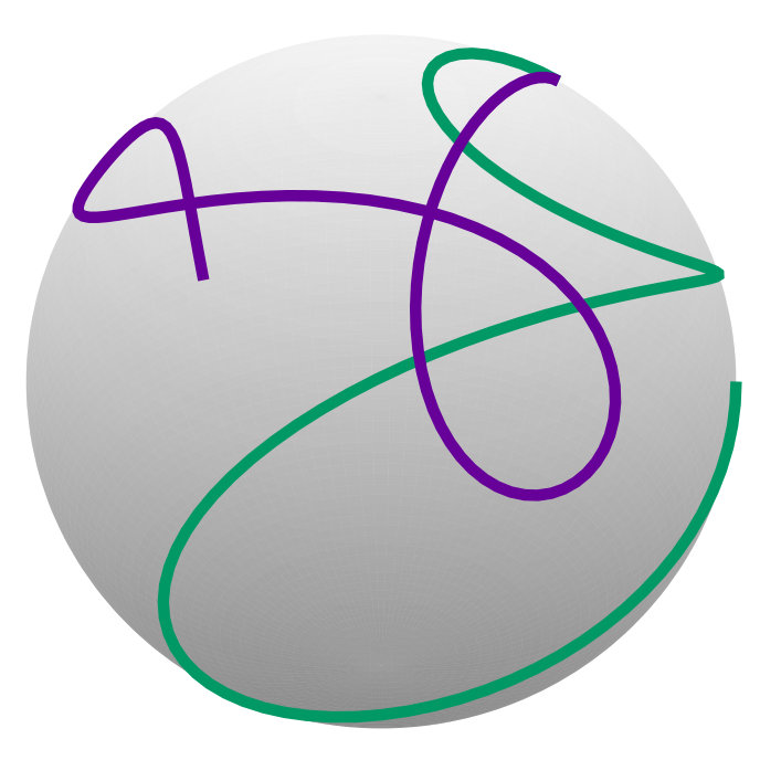 Figure 1
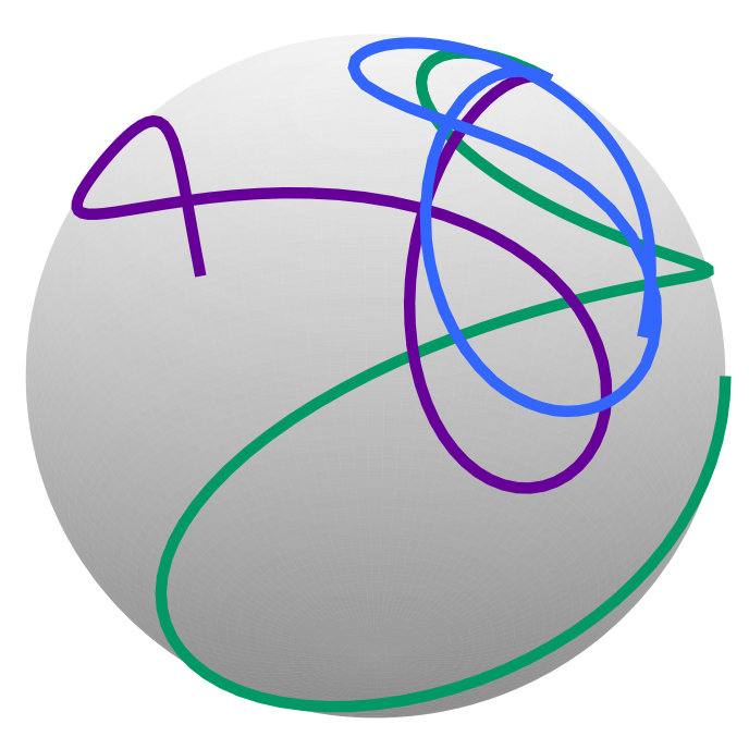 Figure 2
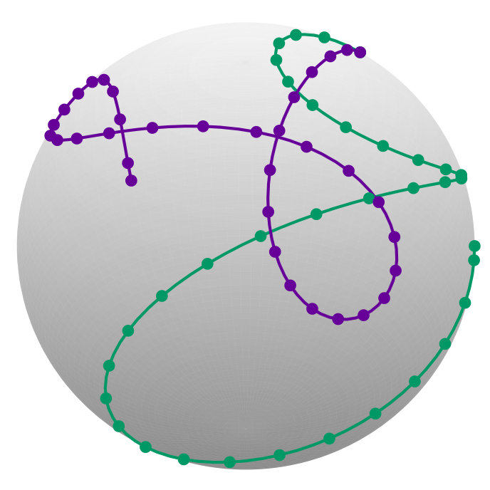 Figure 3
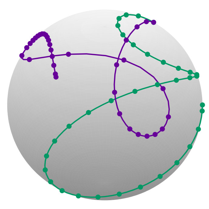 Figure 4
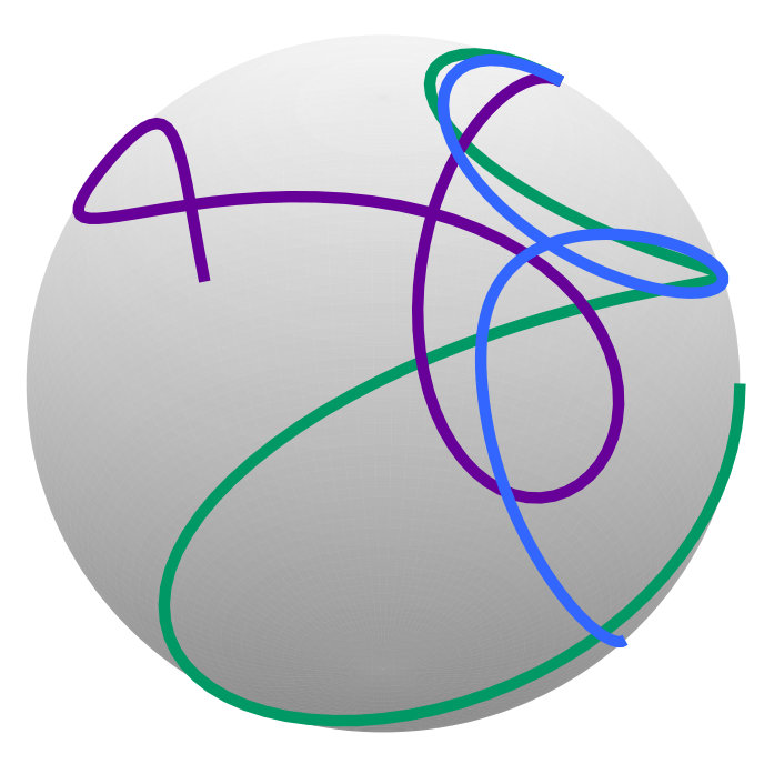 Figure 5
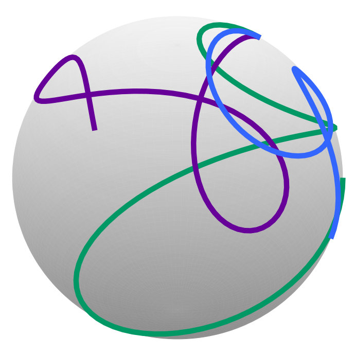 Figure 6
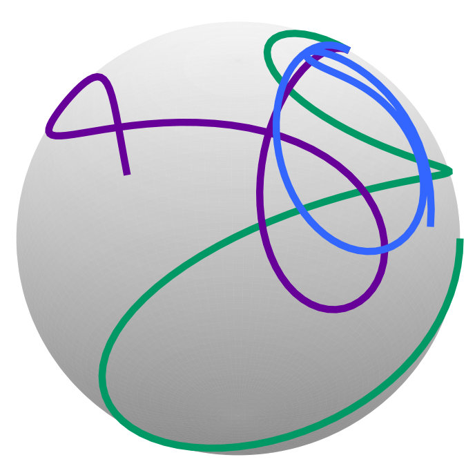 Figure 7
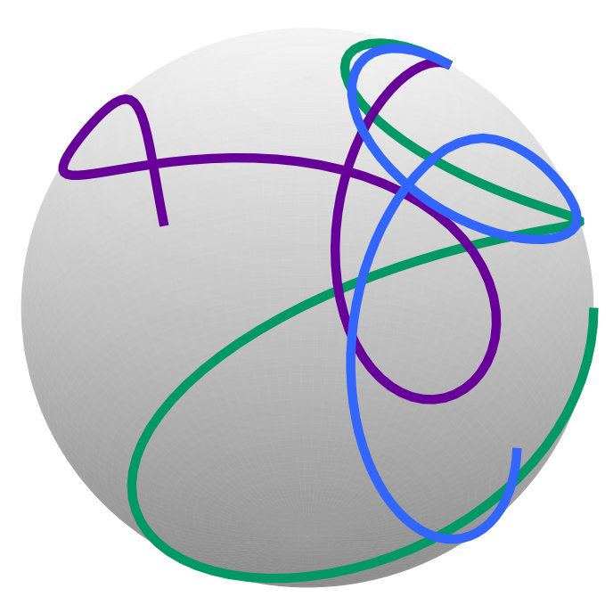 Figure 8
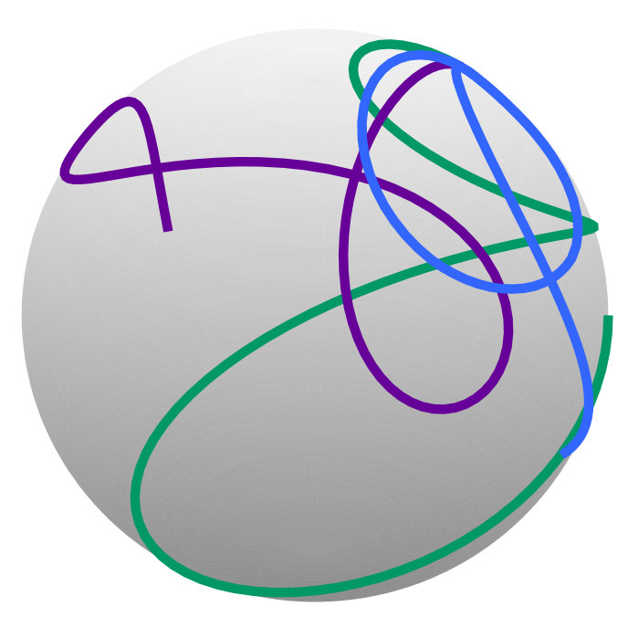 Figure 9
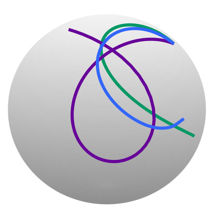 Figure 10
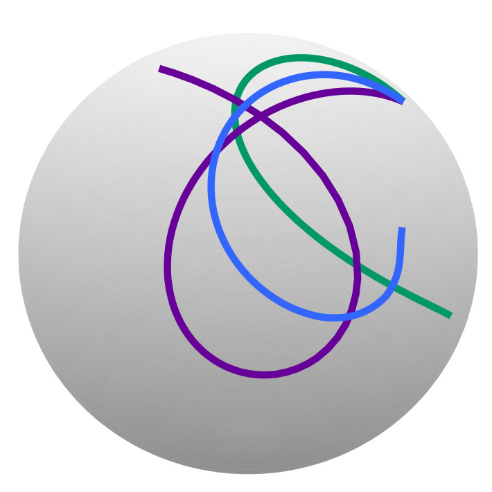 Figure 11
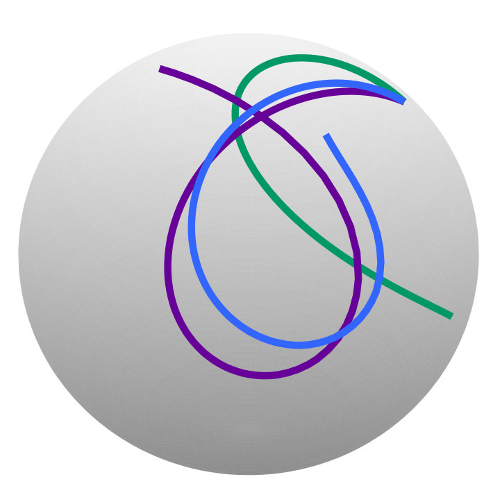 Figure 12
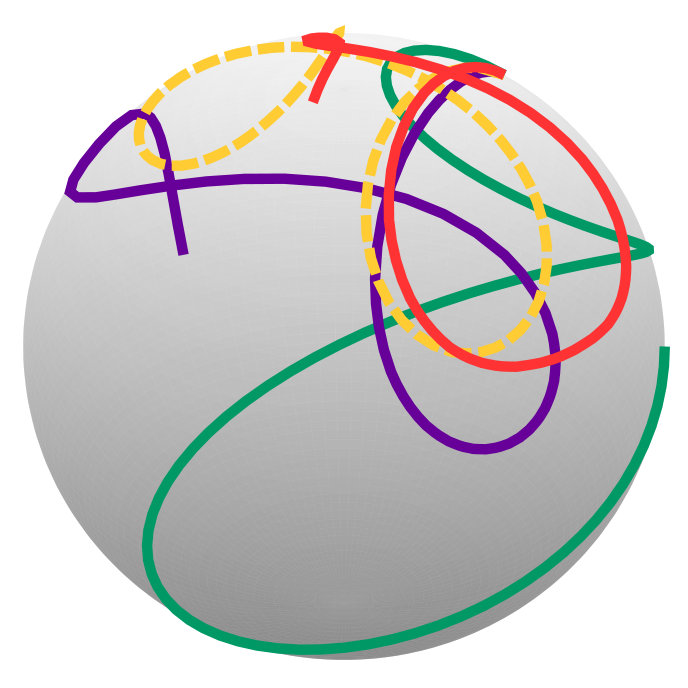 Figure 13
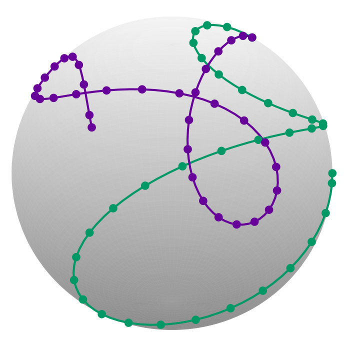 Figure 14
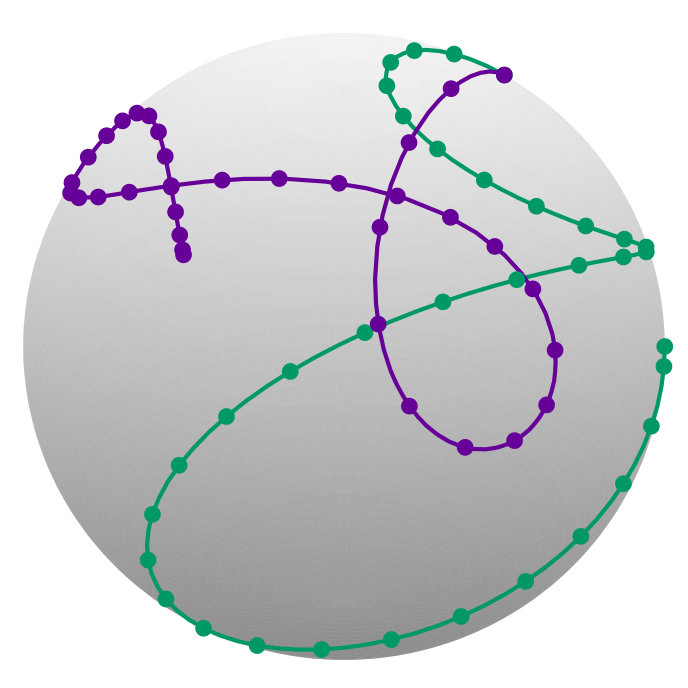 Figure 15
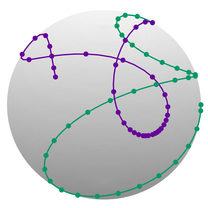 Figure 16
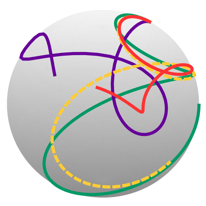 Figure 17
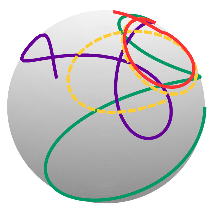 Figure 18
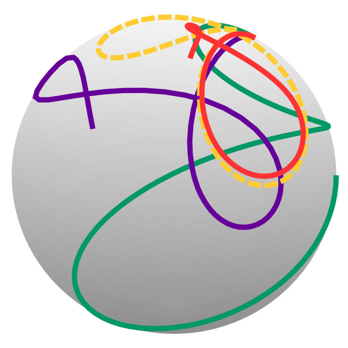 Figure 19
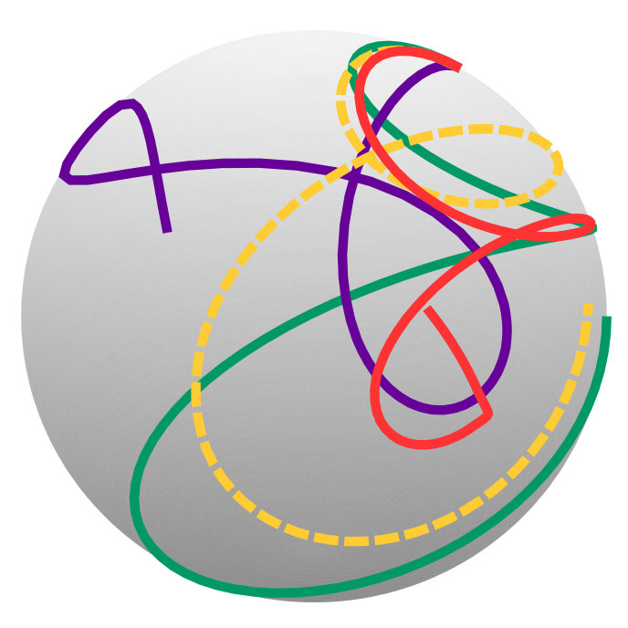 Figure 20
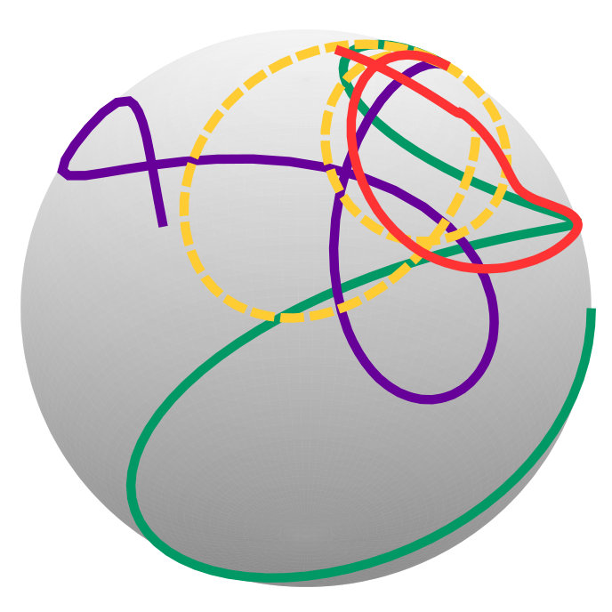 Figure 21
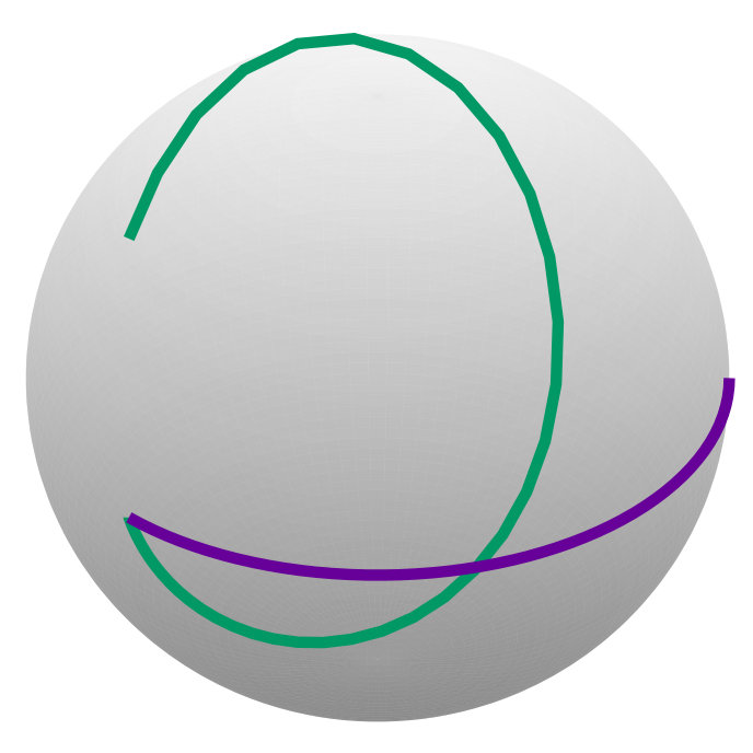 Figure 22
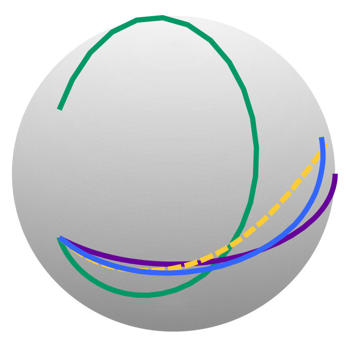 Figure 23
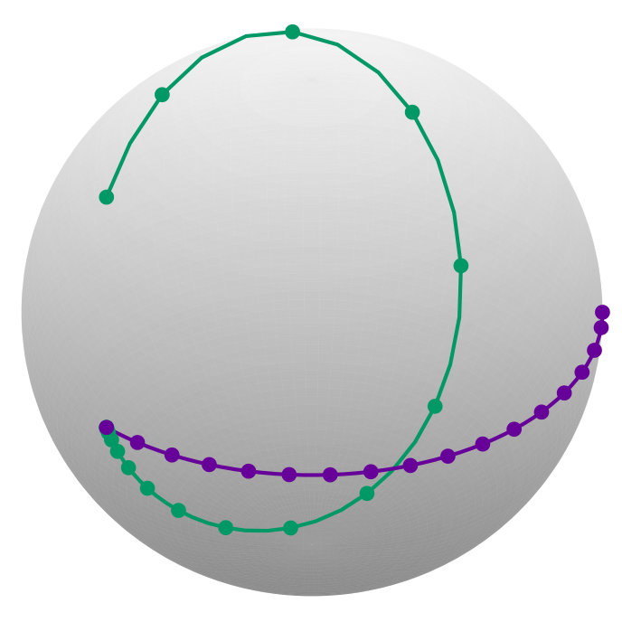 Figure 24
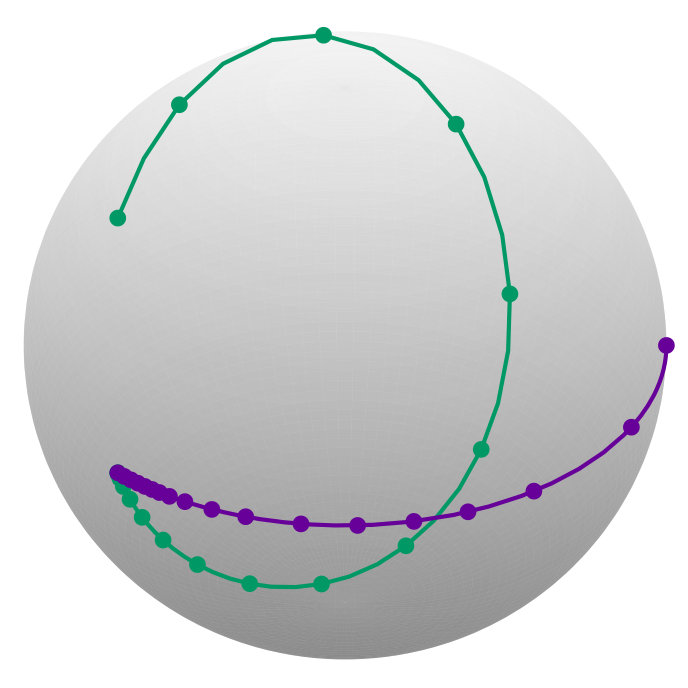 Figure 25
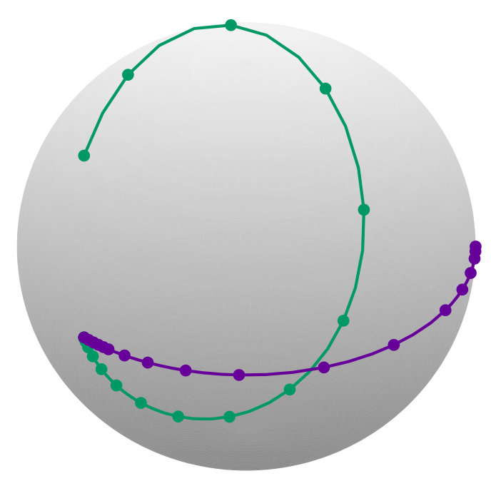 Figure 26
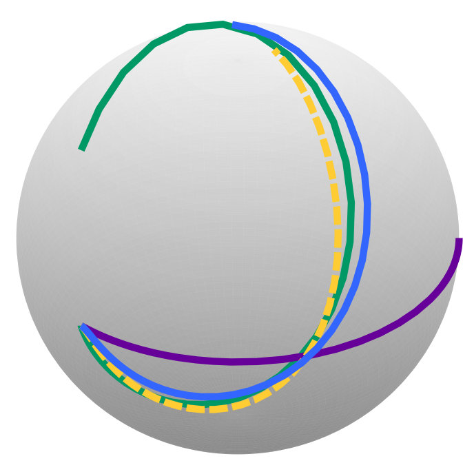 Figure 27
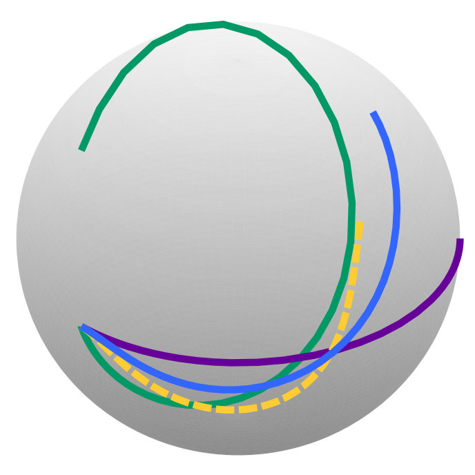 Figure 28
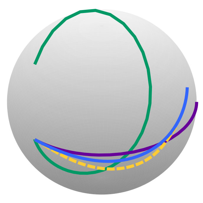 Figure 29
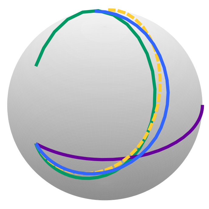 Figure 30
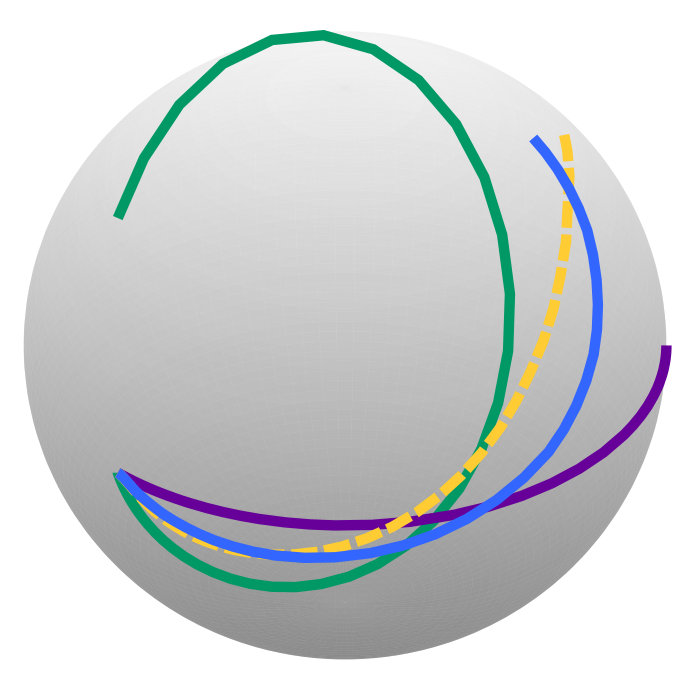 Figure 31
| / | metric on | special decompositions of | -action on |
|---|---|---|---|
| compact | -left invariant, | , the orthogonal | by isometries |
| -biinvariant | complement is -invariant | ||
| compact | -right invariant, | as above | only acts |
| -biinvariant | by isometries | ||
| admits reductive | -right invariant | , is -invariant | not by isometries |
| complement in 444 admits a reductive complement , if is an -invariant subspace and as vector spaces, cf. 3.0.1. Then is a reductive homogeneous space. | , where in general | ||
| -right invariant | but is not | not by isometries | |
| invariant |
Peer Reviews
No public reviews on file for this paper yet. If you reviewed it on a platform where reviews are public (OpenReview, ICLR, NeurIPS, ICML), you can paste yours below so the community can read it here.
Videos
No videos yet. Explain this paper in a talk, walkthrough, or lecture? Add one.
11institutetext: Elena Celledoni 11email: [email protected]: Sølve Eidnes 22email: [email protected] 33institutetext: Alexander Schmeding 33email: [email protected] 44institutetext: NTNU Trondheim, Institutt for matematiske fag, 7491 Trondheim, Norway
Shape analysis on homogeneous spaces: a generalised SRVT framework
E. Celledoni
S. Eidnes
A. Schmeding
Abstract
Shape analysis is ubiquitous in problems of pattern and object recognition and has developed considerably in the last decade. The use of shapes is natural in applications where one wants to compare curves independently of their parametrisation. One computationally efficient approach to shape analysis is based on the Square Root Velocity Transform (SRVT). In this paper we propose a generalised SRVT framework for shapes on homogeneous manifolds. The method opens up for a variety of possibilities based on different choices of Lie group action and giving rise to different Riemannian metrics.
1 Shapes on homogeneous manifolds
Shapes are unparametrised curves, evolving on a vector space, on a Lie group or on a manifold. Shape spaces and spaces of curves are infinite dimensional Riemannian manifolds, whose Riemannian metrics are the essential tool to compare and analyse shapes. By combining infinite dimensional differential geometry, analysis and computational mathematics, shape analysis provides a powerful approach to a variety of applications.
In this paper, we are concerned with the approach to shape analysis based on the Square Root Velocity Transform (SRVT), SKJJ (11). This method is effective and computationally efficient. On vector spaces, the SRVT maps parametrised curves to appropriately scaled tangent vector fields along them. The transformed curves are compared computing geodesics in the metric, and the scaling can be chosen suitably to yield reparametrisation invariance, SKJJ (11), BBMM (14). Notably, applying a (reparametrisation invariant) metric directly on the original parametrised curves is not an option as it leads to vanishing geodesic distance on parametrised curves and on the quotient shape space MM (05); BBHM (12). As an alternative, higher order Sobolev type metrics were proposed MM (06), even though they can be computationally demanding, since computing geodesics in this infinite dimensional Riemannian setting amounts in general to solving numerically partial differential equations. These geodesics are used in practice for finding distances between curves and for interpolation between curves. The SRVT approach, on the other hand, is quite practical because it allows the use of the metric on the transformed curves: distances between curves are just distances of the transformed curves, and geodesics between curves are “straight lines” between the transformed curves. It is also possible to prove that this algorithmic approach corresponds (at least locally) to a particular Sobolev type metric, see BBMM (14); CES (16).
In the present paper we propose a generalisation of the SRVT, from vector spaces and Lie groups, SKJJ (11); BBMM (14), to homogeneous manifolds. This problem has been previously considered for manifold valued curves in SKKS (14); Le (16), but our approach is different, the main idea is to take advantage of the Lie group acting transitively on the homogeneous manifold. The Lie group action allows us to transport derivatives of curves to our choice of base point in the homogeneous manifold. Then this information is lifted to a curve in the Lie algebra. It is natural to require that the lifted curve does not depend on the representative of the class used to pull back the curve to the base point.
The main contribution of this paper is the definition of a generalised square root velocity transform framework using transitive Lie group actions for curves on homogeneous spaces. Different choices of Lie group actions will give rise to different metrics on the infinite dimensional manifold of curves on the homogeneous space, with different properties. These different metrics, their geodesics and associated geometric tools for shape analysis can all be implemented in the computationally advantageous SRVT framework.
We extend previous results for Lie group valued curves and shapes CES (16), to the homogeneous manifold setting. Using ideas from the literature on differential equations on manifolds CO (03), we describe the main tools necessary for the definition of the SRVT and discuss the minimal requirements guaranteeing that the SRVT is well defined, section 2. On a general homogeneous manifold, the SRVT is obtained using a right inverse of the composition of the Lie group action with the evolution operator of the Lie group. If the homogeneous manifold is reductive, there is an explicit way to construct this right inverse (based on a canonical -form for the reductive space, cf. 3.0.3 - 3.0.4), see also MKV (16). We prove smoothness of the defined SRVT in section 2.1. Detailed examples on matrix Lie groups are provided in section 4.
A Riemannian metric on the manifold of curves on the homogeneous space is obtained by pulling back the inner product of curves on the Lie algebra through the SRVT, Theorem 2.11. To ensure that the distance function obtained on the space of parametrised curves descends to a distance function on the shape space, it is necessary to prove equivariance with respect to the group of orientation preserving diffeomorphisms (reparametrization invariance), these results are presented in section 2.3.
For the case of reductive homogeneous spaces, fixed the Lie group action, two different approaches are considered: one obtained pulling back the curves to the Lie algebra (Proposition 3.5) and one obtained pulling back the curves to the reductive subspace (section 3.1.1). The resulting distances are both reparametrization invariant, see Lemmata 2.13 and 3.9. For the second approach it follows similarly to what shown in CES (16) that the geodesic distance is globally defined by the distance, Proposition 3.7. We conjecture that also for general homogeneous manifolds, at least locally, the geodesic distance of the pullback metric is given by the distance of the curves transformed by the SRVT, see end of section 2.2. To illustrate the performance of the proposed approaches we compute geodesics between curves on the -sphere (viewed as a homogeneous space with respect to the canonical -action), see Figure 1 for an example. Numerical experiments show that the two algorithms perform differently when applied to curves on the sphere (section 5).
This work appeared on the arXiv on the 5th of April 2017, later a related but different work from colleagues at Florida State University was completed and posted on the arXiv on the 9th of June 2017. The latter work has now appeared in SKB17b , see also the follow up SKB17a . Moreover, loc.cit. treats quotients by compact subgroups focuses on the existence of optimal reparametrisations.
1.1 Preliminaries and notation
Fix a Lie group with identity element and Lie algebra .111 In this paper we assume all Lie groups and Lie algebras to be finite dimensional. Note however, that many of our techniques carry over to Lie groups modelled on Hilbert spaces, CES (16). Denote by and the right resp. left multiplication by . Let be a closed Lie subgroup of and the quotient with the manifold structure turning into a submersion (see (Glö15a, , Theorem G (b))). Then becomes a homogeneous space for with respect to the (transitive) left action:
[TABLE]
For we write , i.e. (the orbit map of the orbit through ) and .
.
We will consider smooth curves on and describe them using the Lie group action. Namely for we choose a smooth lift of , i.e.:
[TABLE]
In general, there are many different choices for a smooth lifts .222Every homogeneous space is a principal -bundle, whence there are smooth horizontal lifts of smooth curves (depending on some choice of connection, cf. e.g. (OR, 04, Chapter 5.1)). For brevity we will in the following write .
Later on we consider smooth functions on infinite-dimensional manifolds beyond the realm of Banach manifolds. Hence the standard definition for smooth maps (i.e. the derivative as a (continuous) map to a space of continuous operators) breaks down. We base our investigation on the so called Bastiani calculus (see Bas (64)): A map between Fréchet spaces is smooth if all iterated directional derivatives exist and glue together to continuous maps.333In the setting of manifolds on Fréchet spaces (with which we deal here) our setting of calculus is equivalent to the so called convenient calculus (see KM (97)). Convenient calculus defines a map to be smooth if it “maps smooth curves to smooth curves”, i.e. is smooth for any smooth curve . This yields a calculus on infinite-dimensional spaces where smoothness does not necessarily imply continuity (though this does not happen on Fréchet spaces), we refer to KM (97) for a detailed exposition. Note that both calculi can handle smooth maps on intervals , see e.g. (Glö15b, , 1.1) and (KM, 97, Chapter 24).
.
Let be a (possibly infinite-dimensional) manifold. By we denote smooth functions from to . Recall that the topology on these spaces, the compact-open -topology, allows one to control a function and its derivatives. This topology turns into an infinite-dimensional manifold (see e.g. (KM, 97, Section 42)).
Denote by the set of smooth immersions (i.e. smooth curves with ) and recall from (KM, 97, 41.10) that is an open subset of .
.
We further denote by the evolution operator, which is defined as
[TABLE]
and is the tangent of the right translation.Recall from (Glö15b, , Theorem A) that is a diffeomorphism with inverse the right logarithmic derivative
[TABLE]
.
We fix a Riemannian metric on which is right -invariant (i.e. the maps are Riemannian isometries). Since is constructed using the right -action on , an -right invariant metric descends to a Riemannian metric on . We refer to (GHL, 04, Proposition 2.28) for details and will always endow the quotient with this canonical metric to relate the Riemannian geometries.
Hence -right invariance should be seen as a minimal requirement for the metric on . Note that a natural way to obtain (right) invariant metrics is to transport a Hilbert space inner product from the Lie algebra by (right) translation in the group. This method yields a -right invariant metric and we will usually work with such a metric induced by on . Albeit it is very natural, -invariance does not immediately add any benefits. In the following table we record properties of , the Riemannian metric and of the canonical -action on the quotient.
.
Let be a smooth map and denote postcomposition by
[TABLE]
Note that is smooth as a map between (infinite-dimensional) manifolds.
(The SRVT on Lie groups).
For a Lie group with Lie algebra , consider an immersion . The square root velocity transform of is
[TABLE]
where the norm is induced by a right -invariant Riemannian metric, CES (16). The SRVT consists of the composition of three maps:
- •
differentiation ,
- •
transport and
- •
scaling .
The scaling by the square root of the norm of the velocity is crucial to obtain a parametrisation invariant Riemannian metric, see CES (16) and Lemma 2.13.
2 Definition of the SRVT for homogeneous manifolds
Our aim is to construct the SRVT for curves with values in the homogeneous manifold . It was crucial in our investigation of the Lie group case CES (16) that the right-logarithmic derivative inverts the evolution operator, see 1.1.3. To mimic this behaviour we introduce a version of the evolution for homogeneous manifolds.
Definition 2.1.
Fix and denote by all smooth curves with . Then we define
[TABLE]
Remark 2.2.
Fix and and denote by . Then
[TABLE]
Proof.
In fact
[TABLE]
with ∎
Hence we can interpret as a version of the evolution operator for homogeneous manifolds.
Example 2.3.
Consider the two dimensional unit sphere in . Consider the action of on by matrix-vector multiplication: , . Assume the first canonical vector in , then given a curve in the Lie algebra of skew-symmetric matrices , , where satisfies with .
We want to construct a section of the submersion to mimic the construction for Lie groups, see also (CO, 03, Proposition 2.2). As we have seen in the Lie group case, the SRVT factorises into a derivation map, a map transporting the derivative to the Lie algebra and a scaling in the Lie algebra. For homogeneous spaces, we can make sense of this procedure if we can replace the transport from the Lie group case by a map which transports derivatives from the tangent bundle of the homogeneous manifold to the Lie algebra. Thus we search for a map such that the following diagram commutes:
[TABLE]
Moreover, in the Lie group case we see that the mapping maps the submanifold of immersions into the subset . We will require this property in general, as derivatives of immersions should vanish nowhere and this property should be preserved by the transport . The next definition details necessary properties of .
Definition 2.4 (Square root velocity transform).
Let be fixed and define the closed submanifold555As is open and the evaluation map is a submersion, is a closed submanifold of (cf. Glö15a ). of . Assume there is a smooth , such that
[TABLE]
Then we define the square root velocity transform on at , with respect to as
[TABLE]
where is the norm induced by the right invariant Riemannian metric on the Lie algebra. We will see in Lemma 2.9 that is smooth.
The SRVT allows us to transport curves (via ) from the homogeneous manifold to curves with values in a fixed vector space (i.e. the Lie algebra ). The crucial property here is that is a right-inverse of , and we note that our construction depends strongly on the choice of the map .
Example 2.5.
Let be a Lie group and the trivial subgroup (with the Lie group identity). Then is a homogeneous manifold and . Taking , we reproduce the definition of the SRVT on Lie groups 1.1.6. However, contrary to , is not invertible if the subgroup (with ) is non-trivial, but we might still be able to find a right inverse.
Example 2.6.
We have where we have denoted with “” the Euclidean inner product in . Then we can write
[TABLE]
and we can define the map
[TABLE]
For a curve evolving on with , we have so is the right inverse of . The SRVT is then
[TABLE]
and is the norm deduced by the usual Frobenius inner product of matrices (the scaled negative Killing form in see table in example 3.3). See section 4 and 5, for further details and more examples.
The definition of and the SRVT in Definition 2.4 depend on the initial point . In many cases our choices of satisfy (2) for every , i.e. satisfies
[TABLE]
Further, the SRVT also depends on the choice of the left-action . A different action will yield a different SRVT. For example, there are several ways to interpret a Lie group as a homogeneous manifold with respect to different group actions. One of these recovers exactly the SRVT from CES (16) (see Example 2.5). See (MKV, 16, Section 5.1) for more information on Lie groups as homogeneous spaces, e.g. by using the Cartan-Schouten action.
Remark 2.7.
Fix to obtain a smooth map , (Mic, 80, Corollary 11.10 1. and Theorem 11.4). Further we recall from (KM, 97, Theorem 42.17) that . Identifying the tangent space over the constant (taking everything to the unit) we obtain
[TABLE]
If was invertible (which it will not be in general), we could use it to define .
2.1 Smoothness of the SRVT
One of the most important properties of the square root velocity transform is that it allows us to transport curves from the manifold to curves in the Lie algebra, and this operation is smooth and invertible. The details are summarised in the following two lemmata. Following (CES, 16, Lemma 3.9), we consider the smooth scaling maps
[TABLE]
Lemma 2.8.
Fix , then
* is a closed and split submanifold666A submanifold of a (possibly infinite-dimensional) manifold is called split if it is modeled on a closed subvectorspace of the model space of , such that is complemented, i.e. as topological vector spaces (see (Glö15a, , Section 1)). of ,* 2. 2.
* is a smooth surjective submersion.*
Proof.
Note that is the preimage of under the evaluation map
[TABLE]
One can show, similarly to the proof of (CES, 16, Proposition 4.1) that is a submersion.Hence, (Glö15a, , Theorem C) implies that is a closed submanifold of . 2. 2.
Recall that with .
As is a homogeneous space, is a surjective submersion. Hence (OR, 04, Chapter 5.1) implies that is surjective. Further, the Stacey-Roberts Lemma (AS, 17, Lemma 2.4) asserts that is a submersion. Picking , we can also write . Thus is a surjective submersion and
[TABLE]
By (Glö15b, , Theorem C), restricts to a smooth surjective submersion . Finally, since is a diffeomorphism (cf. 1.1.3), is a smooth surjective submersion. ∎
Lemma 2.9.
Fix and let be as in Definition 2.4. Then the square root velocity transform constructed from is a smooth immersion .
Proof.
The map is smooth by Lemma 7.1. Hence on , the restriction of is smooth. As a composition of smooth maps, is also smooth.
Since is a diffeomorphism, it suffices to prove that is an immersion. As we are dealing with infinite-dimensional manifolds, it is not sufficient to prove that the derivative of is injective (which is evident from (2)). Instead we have to construct immersion charts for , i.e. charts in which is conjugate to an inclusion of vector spaces.777See Glö15a for more information on immersions between infinite-dimensional manifolds.
To construct these charts, recall from (2) that is a right-inverse to . In Lemma 2.8 we established that is a surjective submersion which restricts to a submersion by (Glö15a, , Theorem C). Fix and use the submersion charts for . By (Glö15a, , Lemma 1.2) there are open neighborhoods and together with a smooth manifold and a diffeomorphism such that . Thus for a smooth map . Hence induces a diffeomorphism onto the split submanifold . Following (Glö15a, , Lemma 1.13), we see that is an immersion. As was arbitrary, the SRVT is an immersion. ∎
Exploiting that is an immersion, we transport Riemannian structures and distances from to by pullback. Note that the image of the SRVT for a homogeneous space is in general only an immersed submanifold of . For reductive homogeneous spaces, a certain SRVT will always yield a smooth embedding (see Lemma 3.6). We investigate now the Riemannian structure on .
2.2 The Riemannian geometry of the SRVT
As a first step, we construct a Riemannian metric using the metric on .
Definition 2.10.
Endow with the inner product
[TABLE]
where is induced by the right -invariant Riemannian metric of on .
The inner product induces a weak Riemannian metric. The -geodesics are straight lines, i.e. a curve is a -geodesic if and only if for every , is a straight line in the vector space . In Lemma 2.9 the square root velocity transform was identified as an immersion, which we now turn into a Riemannian immersion by pulling back the metric. Arguing as in the proof of (CES, 16, Theorem 3.11) one obtains the following formula for this pullback metric.
Theorem 2.11.
Let and consider , i.e. are curves with . The pullback of the metric on under the SRVT to the manifold of immersions is given by:
[TABLE]
where , is the (transported) unit tangent vector of , and . The pullback of the norm is given by
[TABLE]
The formula for the pullback metric in Theorem 2.11 depends on and its derivative. However, notice that we always obtain a first order Sobolev metric which measures the derivative of the vector field over a curve .
The distance on will now be defined as the geodesic distance of the first order Sobolev metric , i.e. of the pullback of an metric. Thus we just need to pull the geodesic distance on back using the SRVT. But, in general, the geodesic distance of two curves on the submanifold with respect to the metric will not be the distance of the curves (see e.g. (Bru, 16, Section 2)). The question is now, under which conditions is the geodesic distance at least locally given by the distance. Note first that the image of the SRVT will in general not be an open submanifold of (this was the key argument to derive the geodesic distance in (CES, 16, Theorem 3.16)). As a consequence we were unable to derive a general result describing the links between the geodesic distance by on and the SRVT algorithmic approach for homogeneous manifolds. Nonetheless, we conjecture that at least locally the geodesic distance should be given by the distance (note that is an open set, whence the geodesic distance is locally given by the distance). On the other hand, for reductive homogeneous spaces (discussed in Section 3), an auxiliary map can be used to obtain a geodesic distance which globally coincides with the transformed distance.
2.3 Equivariance of the Riemannian metric
Often in applications, one is interested in a metric on the shape space
[TABLE]
where is the group of orientation preserving diffeomorphisms of acting on from the right (cf. BBM (14)). To assure that the distance function descends to a distance function on the shape space, we need to require that it is invariant with respect to the group action.
Definition 2.12.
Let be a metric. Then is reparametrisation invariant if
[TABLE]
In other words is invariant with respect to the diagonal (right) action of on .
Let be equivalence classes and pick arbitrary representatives and . If is a reparametrisation invariant, we define a metric on as
[TABLE]
Since is reparametrisation invariant, the definition of makes sense (cf. (CES, 16, Lemma 3.4)). To obtain a metric on , we need reparametrisation invairance of
[TABLE]
Lemma 2.13.
Let be the square root velocity transform with respect to and . Then is reparametrisation invariant if is a -valued -form on , e.g. if for a -valued -form on .
Proof.
Consider and . Then a computation yields
[TABLE]
where we have used that is fibre-wise linear as a -form. Thus we can now compute
[TABLE]
The condition on from Lemma 2.13 is satisfied in all examples of the SRVT considered in the present paper. For example, for a reductive homogeneous case (see Section 3), we can always choose as the pushforward of a -valued -form.
3 SRVT for curves in reductive homogeneous spaces
A fundamental problem in our approach to shape spaces with values in homogeneous spaces is that we need to somehow lift curves from the homogeneous space to the Lie group. Ideally, this lifting process should be compatible with the Riemannian metrics on the spaces. Note that for our purposes it suffices to lift the derivatives of smooth curves to curves in the Lie algebra of the Lie group. Hence we need a suitable Lie algebra valued -form, which turns out to exist for reductive homogeneous spaces, cf. e.g. (KN, 69, Chapter X) (see also MKV (16) for a recent account)
.
Recall that , where denotes conjugation . Suppose is a subspace of such that
Let be the inverse of . Identify and observe that induces an isomorphism .
By definition holds for all . Now the group actions of on itself by left and right multiplication commute and we observe that
[TABLE]
.
We will from now on assume that is a reductive homogeneous manifold. This means that the subalgebra admits a reductive complement, i.e. a vector subspace such that
[TABLE]
If it exists, a reductive complement will in general not be unique. However, we choose and fix a reductive complement for .
.
As a reductive complement, is closed with respect to the adjoint action of . Hence one deduces (cf. (MKV, 16, Lemma 4.6) for a proof) that is -invariant with respect to the adjoint action, i.e.
[TABLE]
Thus the following map is well-defined:
[TABLE]
From the definition it is clear that is a smooth -valued -form on . Moreover, is even -equivariant with respect to the canonical and adjoint action:
[TABLE]
Note that depends by construction on our choice of reductive complement . However, we will suppress this dependence in the notation. As noted in (MKV, 16, Section 4.2), the -forms correspond bijectively to reductive structures on .888Note that there might be different reductive structures on a homogeneous manifold. We refer to (MKV, 16, Section 5.1) for examples and further references.
.
Let be the -form constructed in 3.0.3. Then we define the map
[TABLE]
Note first that is smooth by (KM, 97, Theorem 42.13). We will prove that indeed satisfies (2) and (3), whence yields an SRVT as in 2.4.
To motivate the computations, let us investigate an important special case.
Example 3.1.
Similarly to example 2.5, let be a Banach Lie group and the trivial subgroup. Then can be viewed as a reductive homogeneous manifold with , and . From the definition of we obtain where denotes the right Maurer-Cartan form, (KM, 97, Section 38) or (MKV, 16, Section 5.1). In particular, for we have (right logarithmic derivative). As we have for a curve starting at .
The SRVT for reductive spaces coincides thus with the SRVT for Lie group valued shape spaces as outlined in 1.1.6.
Albeit Example 3.1 is quite trivial as a homogeneous space, it highlights a general principle of the construction for reductive homogeneous spaces.
Remark 3.2.
We here provide an alternative interpretation for : A smooth curve admits a smooth horizontal lift depending on a choice of connection for the principal bundle (OR, 04, Chapter 5.1). For a reductive homogeneous manifold we construct a horizontal lift using the canonical invariant connection (depending on the reductive complement, see (KN, 69, X.2)). Now we take the (right) Darboux derivative (aka right logarithmic derivative) of (see (Sha, 97, 3.§5)). Then unraveling the definitions similar to Examples 2.5 and 3.1, one can show that holds for the -form as in 3.0.4. Thus for a reductive homogeneous space the proposed SRVT can be viewed (up to scaling) as the Darboux derivative of a horizontal lift of a curve in . Note that this interpretation justifies again to view as a generalised version of the evolution operator (which inverts the right logarithmic derivative, see Remark 2.2).
A rich source for reductive homogeneous spaces are quotients of semisimple Lie groups. We recall now some of the main examples.
Example 3.3.
Let be a semisimple Lie group and a Lie subgroup of which is also semisimple. Then the homogeneous space is reductive. A reductive complement of in is the orthogonal complement with respect to the Cartan-Killing form on (recall that the Killing form of a semisimple Lie algebra is non-degenerate by Cartan’s criterion (Kna, 02, I.§7 Theorem 1.45)). For example, this occurs for and or and (where ), since by (Kna, 02, I.§8 and I.§18) the following properties hold:
[TABLE]
Here Tr denotes the trace of a matrix. All main examples in this paper are reductive.
Proposition 3.4.
Let be a reductive homogeneous space, , and as in 3.0.4. Consider . Then
[TABLE]
Proof.
As a shorthand write . We establish in Lemma 7.2 the identity
[TABLE]
Let now with . Then we obtain and
[TABLE]
Recall from (Glö15b, , 1.16) that for a Lie group morphism one has the identity . By definition, , where denotes the conjugation morphism. Insert this into the above equation:
[TABLE]
In passing to the second line we used that left and right multiplication maps commute and that . ∎
Proposition 3.5.
Let be a reductive homogeneous space, , and as in 3.0.4. Then satisfies (2) and (3), whence for a reductive homogeneous space we can define the SRVT as
[TABLE]
Proof.
In Proposition 3.4 we have already established (2). To see that (3) also holds for , observe first that for , we have . Since and are linear isomorphisms, we see that if and only if . As is post-composition by , satisfies (3). ∎
3.1 Riemannian geometry and the reductive SRVT
In the reductive space case, it is easier to describe the image of the square root velocity transform. It turns out that the image is a split submanifold with a global chart. Using this chart, we can also obtain information on the geodesic distance.
The idea is to transform the image of the SRVT such that it becomes , where is again the reductive complement. Pick and use the adjoint action of and the evolution to define
[TABLE]
where the dot denotes pointwise application of the linear map . Then is a diffeomorphism with inverse (see Lemma 7.4). We will now see that maps the image of the SRVT to .
Lemma 3.6.
Choose in the reductive homogeneous space , and let and , be as in Proposition 3.4. Then is a split submanifold of modelled on and is a smooth embedding. In particular, is a split submanifold of and is a smooth embedding.
Proof.
As , we have . Thus is a closed and split submanifold of . Fix with and note that restricts to a diffeomorphism by Lemma 7.4. Now as (cf. Lemma 7.5), the image is a closed and split submanifold of . Further, we deduce from Lemma 7.5 that is smooth with . As also , we see that is a diffeomorphism onto its image. Thus is indeed a smooth embedding.
Since the scaling maps are diffeomorphisms , the assertions on the image of and on follow directly from the assertions on . ∎
(Reductive SRVT).
Let be a reductive homogeneous space with reductive complement and be constructed with respect to the -form from 3.0.3. Then (see Appendix 7.0.1). Now one constructs a version of the SRVT for reductive spaces via
[TABLE]
We call this map reductive SRVT, to distinguish it from the usual SRVT. Contrary to the SRVT, the reductive SRVT will go into the reductive complement, but it will not be a section of . Instead it is a section of . Finally, we note that by construction (cf. Lemma 7.4) the image of the reductive SRVT is .
Arguing as in Theorem 2.11, we also obtain a first order Sobolev metric by pullback with the reductive SRVT. In general this Riemannian metric will not coincide with the pullback metric obtained from the SRVT. The advantage of the reductive SRVT is that we have full control over its image, which happens to be an open subset (of a subspace of ). Since with respect to the inner product is a flat space (in the sense of Riemannian geometry), it follows that at least locally the geodesic distance on the image of the SRVT is given by the distance
[TABLE]
However, we argue as in (CES, 16, Theorem 3.16) to obtain the following result.
Proposition 3.7.
If , then the geodesic distance of coincides with the distance. In this case the geodesic distance on induced by the pullback metric (5) (with respect to the reductive SRVT) is given by
Note that the modification by the reductive SRVT is highly non-linear, e.g. in the Lie group case, Example 3.1, we obtain:
Example 3.8.
Let be a Lie group, and . Then
[TABLE]
Recall from (KM, 97, 38.4) that . In the Lie group case, the reductive SRVT modifies the formulae to compute distances and interpolations between the pointwise inverses of curves instead of the curves themselves. In particular, this shows that the reductive SRVT will not be a section of .
In particular, we have to prove a version of Lemma 2.13 for the reductive SRVT.
Lemma 3.9.
For a reductive space, is reparametrisation invariant.
Proof.
For we use instead of . Consider and to compute as in Lemma 2.13: . Now
[TABLE]
follows from (KM, 97, p. 411). Linearity of the adjoint action yields . Inserting this in (9) yields reparametrisation invariance. ∎
4 The SRVT on matrix Lie groups
In order to illustrate our definition of the SRVT in different instances of homogeneous manifolds, we consider in what follows two examples of quotients of finite dimensional matrix Lie groups (for and ):
(see 4.3).
- 2.
(see 4.2).
Note that in both cases the quotients are reductive homogeneous spaces. To prepare our investigation, we will now collect some information on relevant tangent spaces for the matrix Lie groups. These examples are relevant in applications AMS (07).
4.1 Tangent space of and tangent map of
For and finite dimensional (matrix) Lie groups, we here describe the tangent space of at a prescribed point and the tangent mapping of the canonical projection . We have seen that any curve on , , can be expressed non-uniquely by means of a curve on the Lie group . For matrix Lie groups, the elements of are equivalence classes of matrices. Let the elements of , , be matrices, then the group multiplication coincides with matrix multiplication. We identify elements of with matrices
[TABLE]
We obtain , , by differentiating . Assuming , , , we have
[TABLE]
Assuming , where , , and assuming also that , in analogy to (32), we get
[TABLE]
so we obtain
[TABLE]
which gives a description of the tangent vector as well as the characterisation of for matrix Lie groups. Suppose that we fix a complementary subspace of , , then there is a unique isotropy element such that .
Repeating this procedure for each value of along a curve , we can assume and , with , , such that , then we can define
[TABLE]
This map corresponds to the map of 3.0.4 with as described in 3.0.3. If is reductive, this map is well defined (independently of the choice of representative of ). We refer to Table 1 for different, possible choices of and their implications. In the following examples is reductive and is compact.
4.2 SRVT on the Stiefel manifold: .
In this section we consider the case when and , where the elements of are of the type (11) with a orthogonal matrix with determinant equal to . We consider the canonical left action of on the quotient . This homogeneous manifold can be identified with the Stiefel manifold, , i.e. the set of -orthonormal frames in (real matrices with orthonormal columns). We will in the following denote by the elements of where we have collected in the first orthonormal columns and in the last . Multiplication from the right by an arbitrary element in the isotropy subgroup gives , leaving the first columns unchanged and orthonormal to the last , for all choices of . Here alone represents the whole coset of . When thought of as a map from to , the projection is
[TABLE]
Otherwise, when thought of as a map from , the canonical projection conveniently becomes where is the matrix whose columns are the first columns of the identity matrix. The equivalence class of the group identity element is identified with the matrix . Similarly the tangent mapping of the projection ,
[TABLE]
with , and ), can be realised as
[TABLE]
while by multiplication from the right by , and
[TABLE]
Alternatively, a characterisation of tangent vectors can be obtained by differentiation of curves on . We have then that
[TABLE]
Proposition 4.1.
CO (03*)** Any tangent vector at can be written as *
[TABLE]
And notice that replacing with , where is an arbitrary symmetric matrix, does not affect (15).
We proceed by using the representation (15) of and the framework described in Definition 2.4 for defining an SRVT on the Stiefel manifold. Consider
[TABLE]
The SRVT of a curve on the Stiefel manifold is a curve on defined by
[TABLE]
As the Stiefel manifold is a reductive homogeneous space, we can define a reductive SRVT in this case. Denoting with a representative in of the equivalence class identified by on , we observe that
[TABLE]
Assuming the right invariant metric on is the negative Killing form, then we observe that belongs to the orthogonal complement of the subalgebra in with respect to this inner product. As stated in Table 1, this orthogonal complement is the reductive complement, i.e. , and . The elements of such an orthogonal complement are matrices of the form
[TABLE]
with and an arbitrary matrix. Consider the maps
[TABLE]
and we observe that . Then the reductive SRVT is
[TABLE]
4.3 SRVT on the Grassmann manifold: .
In this section we consider the case when and where the elements of are of the type
[TABLE]
with a matrix and an matrix, both orthogonal with determinant equal to . We consider the canonical left action of on the quotient . This homogeneous manifold can be identified with a quotient of the Stiefel manifold with equivalence classes . We denote such a manifold here with 999An alternative representation of is given by considering symmetric matrices , , with and , HL (07).. The reductive subspace is with elements as in (20) but with . Imposing a choice of isotropy such that leads to the following characterisation of tangent vectors.
Proposition 4.2.
Any tangent vector at is an matrix such that , and can be expressed in the form (15) with .
The proof follows from (12) assuming , and of the form (24), imposing the stated choice of isotropy, and projecting the resulting curves on by post-multiplication by .
We proceed by using (15) but with . Define as in (18) with the identity map . Suppose that is a curve on the Grassmann manifold, then the SRVT of is a curve on and takes the form (19) which here becomes
[TABLE]
The reductive SRVT is defined by (23) with
[TABLE]
and as in (22), which implies .
5 Numerical experiments
To demonstrate an application of the SRVT introduced in this paper, we present a simple example of interpolation between two curves on the unit -sphere. In the following we describe some implementation details for this example.
(Preliminaries).
We will use Rodrigues’ formula for the Lie group exponential,
[TABLE]
where defines an isomorphism between vectors in and skew-symmetric matrices in .
(Interpolated curves).
Given a continuous curve on the Stiefel manifold , which is diffeomorphic to , we replace with the curve interpolating between values , with , as follows:
[TABLE]
where is the characteristic function, is the Lie group exponential, and are approximations to found by solving the equations
[TABLE]
The , , can be found explicitly, by a simple calculation. We observe that if , then . By (28), we have that , where the last equality follows because we assume the sphere to have radius , and so . Using Rodrigues’ formula, from (27) we obtain
[TABLE]
Thus and so leading to
[TABLE]
Inserting this into (26) gives
[TABLE]
(The SRVT and its inverse).
By Definition 2.4 and formulae (17), (18) and (19), the SRVT of the curve (29) is a piecewise constant function in , taking values , where is given by
[TABLE]
Here the norm is induced by the negative (scaled) Killing form, which for skew-symmetric matrices corresponds to the Frobenius inner product, .
The inverse SRVT is then given by (29), with
[TABLE]
(The reductive SRVT).
Since , the reductive SRVT (3.1.1) becomes then
[TABLE]
with
[TABLE]
where can be found e.g. by -factorization of .
•
(Curve blending on the 2-sphere).
We wish to compute the geodesic in the shape space of curves on the sphere between the two curves and . Following CES (16), we use a dynamic programming algorithm to solve the optimization problem (7) (see SKK (03); BEG (15) for a detailed description on the use of dynamic programming for shapes):
With this approach, we reparametrise optimally the curve while minimizing its distance to . This distance is measured by taking the norm of in the Lie algebra. In the discrete case, this reparametrisation yields an optimal set of grid points , where , from which we find by (29). See CES (16) for further details.
We interpolate between and by performing a linear convex combination of their SRV transforms and , and then by taking the inverse SRVT of the result. We obtain
[TABLE]
Examples are reported in Figures 2, 3 and 4, where interpolation between two curves is performed with and without reparametrisation. We show curves resulting from using both (30) and (31), and compare these to the results obtained when employing the SRVT introduced in CES (16) on curves in which are then traced out by a vector in to match the curves in studied here.
(Conclusions).
We have proposed generalisations of the SRVT approach to curves and shapes evolving on homogenous manifolds using Lie group actions. Different Lie group actions lead to different Riemannian metrics in the infinite dimensional manifolds of curves and shapes opening up for a variety of possibilities which can all be implemented in the same generalised SRVT framework. We have presented only a few preliminary examples here, and further tests and analysis will be the subject of future work. A number of open questions related to the properties of the pullback metrics through the SRVT, to the performance of the algorithms when using different Lie group actions, to the comparison of the SRVT and the reductive SRVT and to the implementation of the approach in examples of non reductive homogeneous manifolds will be addressed in future research.
6 Acknowledgment
This work was supported by the Norwegian Research Council, and by the European Union’s Horizon 2020 research and innovation programme under the Marie Sklodowska-Curie, grant agreement No. 691070.
7 Appendix
(Auxiliary results for Section 3).
Lemma 7.1.
For the homogeneous space with projection the derivation map is smooth.
Proof.
The map is a smooth group homomorphism by (Glö15b, , Lemma 2.1). As is a smooth submersion, is a smooth submersion (AS, 17, Lemma 2.4). Write , whence by (Glö15a, , Lemma 1.8) is smooth. ∎
Lemma 7.2.
With The identity (10) holds.
Proof.
Let be smooth with and choose smooth with and . Set . It suffices to prove that for all . Then and the assertion follows.
As , we only have to prove that vanishes everywhere to obtain . Before we compute the derivative of , let us first collect some facts concerning the logarithmic derivatives and . By definition . Further,(KM, 97, Lemma 38.1) yields for smooth :
[TABLE]
Recall that by definition, (here is used). Inserting this into the above equation we obtain
[TABLE]
Observe that since . As is a section of , . Summing up
[TABLE]
(A chart for the image of the SRVT).
Let be a Lie group with Lie algebra . Using the adjoint action of on and the evolution , we define the map
[TABLE]
where the dot denotes pointwise application of the linear map . Observe that (co)restricts to a mapping .
Lemma 7.3.
The map is a smooth involution.
Proof.
To establish smoothness of , consider the commutative diagram
[TABLE]
As is smooth, so is (cf. (Glö15b, , Proof of Proposition 6.2)) and is smooth as a composition of smooth maps. Compute for
[TABLE]
To see that , we prove that is a constant path. Recall that and are smooth paths starting at the identity in . Hence it suffices to prove . To this end, apply the product formula (32) and :
[TABLE]
To account for the initial point , fix and define
[TABLE]
For in the center of , holds, but in general will not be an involution.
Lemma 7.4.
For each , the map is a diffeomorphism with inverse .
Proof.
From the definition of and Lemma 7.3, it is clear that is a smooth diffeomorphism. We use that is a group morphism and compute
[TABLE]
Here we used that ∎
Lemma 7.5.
Fix and choose with . Assume that is reductive with , then
[TABLE]
With as in 3.0.4 the formula holds.
Proof.
Consider and recall from Proposition 3.4 the identity . Choose as a smooth lift of to and compute as follows:
[TABLE]
Conversely, let us show that is contained in the image of . To this end, consider for . We compute
[TABLE]
Since is a diffeomorphism, is an immersion if and only if the curve has a non-vanishing derivative everywhere. Recall from the proof of Lemma 7.3 that , whence we compute the derivative
[TABLE]
In passing to the last line, we used that commutes with the left action. Since is an isomorphism, vanishes if and only if . However, , whence and we can apply to . A combination of (34) and (35) yields With , this yields
[TABLE]
Note that as , we have . ∎
The reference list from the paper itself. Each links out to its DOI / PubMed record.
- 1AMS (07) Absil, P.-A., Mahony, R. and Sepulchre, R. Optimization algorithms on matrix manifolds (Princeton University Press, 2007)
- 2AS (17) Amiri, H. and Schmeding, A. A differentiable monoid of smooth maps on Lie groupoids 2017. ar Xiv:1706.04816 v 1
- 3Bas (64) Bastiani, A. Applications différentiables et variétés différentiables de dimension infinie . J. Analyse Math. 13 (1964):1–114
- 4BBHM (12) Bauer, M., Bruveris, M., Harms, P. and Michor, P. W. Vanishing geodesic distance for the Riemannian metric with geodesic equation the Kd V-equation . Ann. Global Anal. Geom. 41 (2012)(4):461–472
- 5BBM (14) Bauer, M., Bruveris, M. and Michor, P. W. Overview of the Geometries of Shape Spaces and Diffeomorphism Groups . Journal of Mathematical Imaging and Vision (2014):1–38
- 6BBMM (14) Bauer, M., Bruveris, M., Marsland, S. and Michor, P. W. Constructing reparameterization invariant metrics on spaces of plane curves . Differential Geom. Appl. 34 (2014):139–165
- 7BEG (15) Bauer, M., Eslitzbichler, M. and Grasmair, M. Landmark-guided elastic shape analysis of human character motions 2015
- 8Bru (16) Bruveris, M. Optimal reparametrizations in the square root velocity framework . SIAM J. Math. Anal. 48 (2016)(6):4335–4354