Roles of energy eigenstates and eigenvalues in equilibration of isolated quantum systems
Shaoqi Zhu, Biao Wu

TL;DR
This paper investigates how energy eigenstates and eigenvalues differently influence the equilibration of isolated quantum systems, revealing that non-integrable models exhibit non-degenerate energies and 'random' eigenstates that promote equilibration.
Contribution
It demonstrates the distinct roles of eigen-energies and eigenstates in quantum equilibration, highlighting the importance of non-degeneracy and randomness in non-integrable models.
Findings
Non-integrable models have non-degenerate eigen-energies facilitating rare revivals.
Energy eigenstates in non-integrable models suppress fluctuations in equilibrium.
Quantum entropy confirms the 'random' nature of eigenstates, supporting Berry's conjecture.
Abstract
We show that eigen-energies and energy eigenstates play different roles in the equilibration process of an isolated quantum system. Their roles are revealed numerically by exchanging the eigen-energies between an integrable model and a non-integrable model. We ?find that the structure of eigenenergies of a non-integrable model characterized by non-degeneracy ensures that quantum revival occurs rarely whereas the energy eigenstates of a non-integrable model suppress the fluctuations for the equilibrated quantum state. Our study is aided with a quantum entropy that describes how randomly a wave function is distributed in quantum phase space. We also demonstrate with this quantum entropy the validity of Berry's conjecture for energy eigenstates. This implies that the energy eigenstates of a non-integrable model appear indeed "random".
Click any figure to enlarge with its caption.
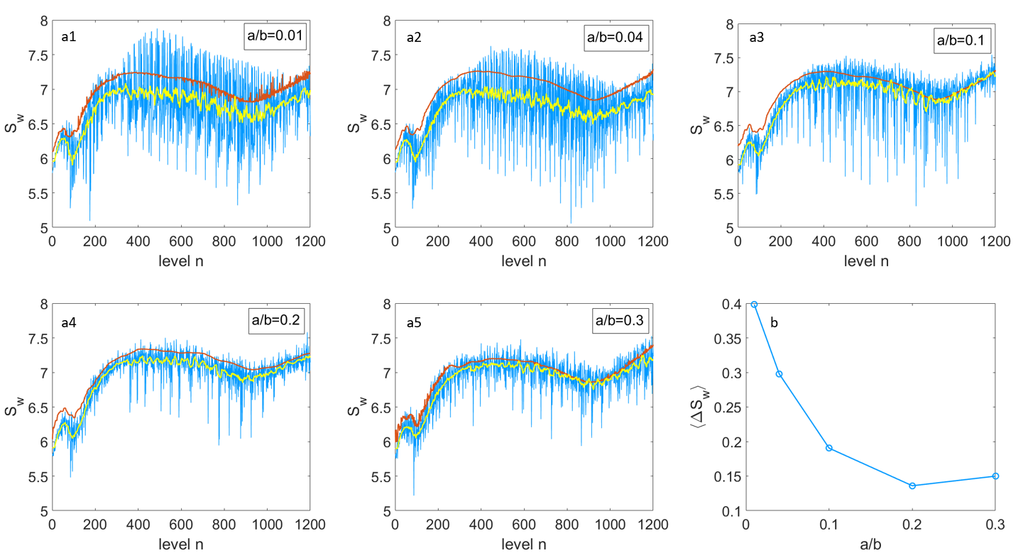 Figure 1
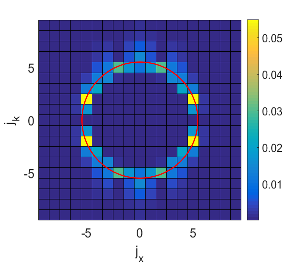 Figure 2
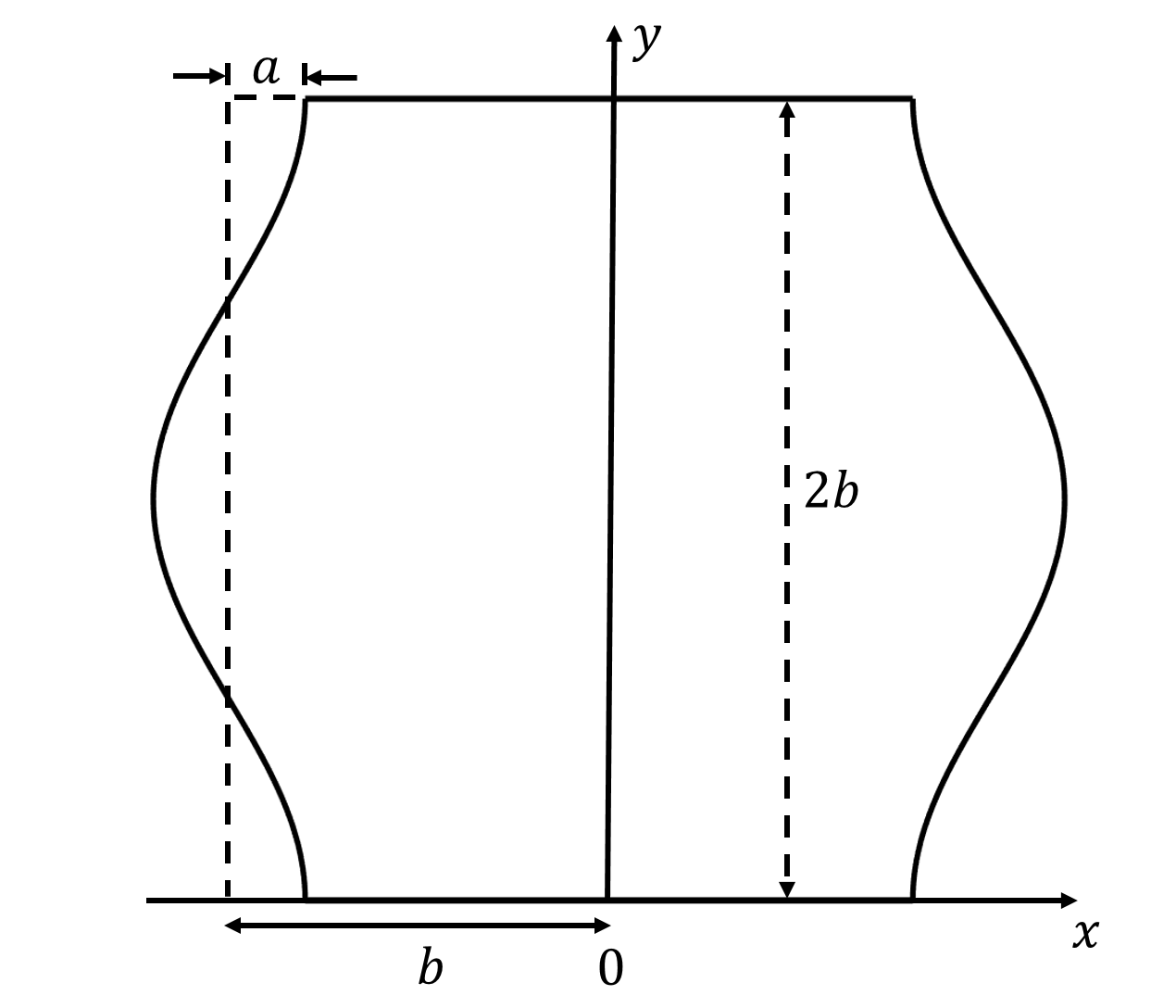 Figure 3
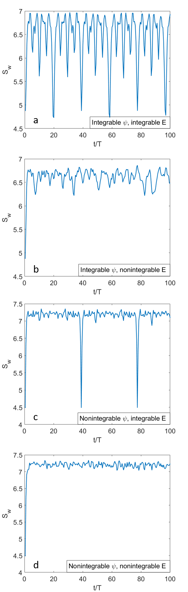 Figure 4
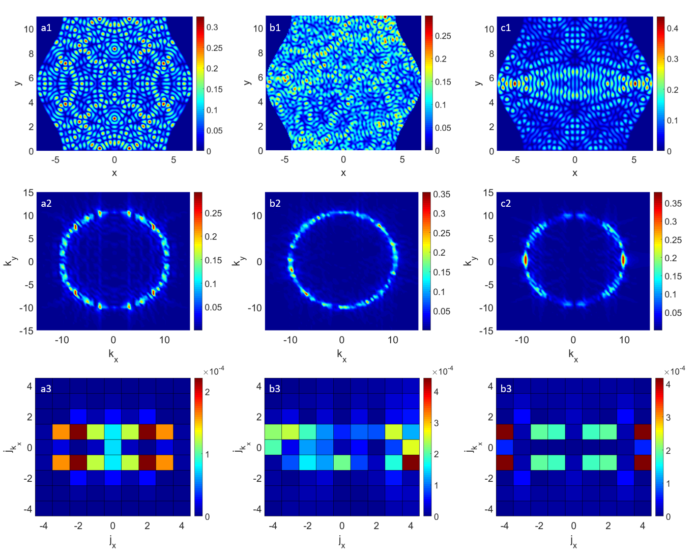 Figure 5
Peer Reviews
No public reviews on file for this paper yet. If you reviewed it on a platform where reviews are public (OpenReview, ICLR, NeurIPS, ICML), you can paste yours below so the community can read it here.
Videos
No videos yet. Explain this paper in a talk, walkthrough, or lecture? Add one.
Roles of energy eigenstates and eigenvalues in equilibration of isolated quantum systems
Shaoqi Zhu(朱少奇)
International Center for Quantum Materials, Peking University, 100871, Beijing, China
Biao Wu(吴飙)
International Center for Quantum Materials, Peking University, 100871, Beijing, China
Collaborative Innovation Center of Quantum Matter, Beijing 100871, China
Wilczek Quantum Center, Department of Physics and Astronomy, Shanghai Jiao Tong University, Shanghai 200240, China
Abstract
We show that eigen-energies and energy eigenstates play different roles in the equilibration process of an isolated quantum system. Their roles are revealed numerically by exchanging the eigen-energies between an integrable model and a non-integrable model. We find that the structure of eigen-energies of a non-integrable model characterized by non-degeneracy ensures that quantum revival occurs rarely whereas the energy eigenstates of a non-integrable model suppress the fluctuations for the equilibrated quantum state. Our study is aided with a quantum entropy that describes how randomly a wave function is distributed in quantum phase space. We also demonstrate with this quantum entropy the validity of Berry’s conjecture for energy eigenstates. This implies that the energy eigenstates of a non-integrable model appear indeed “random”.
I introduction
How equilibration is achieved in an isolated quantum system is a fundamental issue regarding the foundation of quantum statistical mechanics. This issue has intrigued many physicists von Neumann (1929, 2010); Goldstein et al. (2010). In standard textbooks on quantum statistical physics, one just assumes that quantum equilibration can be achieved and assign the equilibrated state certain properties with postulates, such as equal a priori probability, to establish micro-canonical ensemble. In his well-known textbook Huang (1987), Huang states, ”The postulates of quantum statistical mechanics are to be regarded as working hypotheses whose justification lies in the fact that they lead to results in agreement with experiments. Such a point of view is not entirely satisfactory, because these postulates cannot be independent of, and should be derivable from, the quantum mechanics of molecular systems”. This issue has recently received renewed interests Goldstein et al. (2006a); Popescu et al. (2006); Reimann (2008); Goldstein et al. (2006b); Linden et al. (2009); Fine (2009); Ikeda et al. (2011); Yukalov (2011); Gogolin et al. (2011); Riera et al. (2012); Short (2011); Reimann and Kastner (2012); Sugiura and Shimizu (2012, 2013); Zhuang and Wu (2014, 2013); Han and Wu (2015); Zhang et al. (2016) due to experimental developments Smith et al. (2013); Niu et al. (2016)
In 1929 von Neumann addressed this fundamental issue by proving quantum ergodic theorem and quantum theorem von Neumann (1929); Goldstein et al. (2010), where he claimed, “in quantum mechanics one can prove the ergodic theorem and the H-theorem in full rigor and without disorder assumptions; thus, the applicability of the statistical-mechanical methods to thermodynamics is guaranteed without relying on any further hypotheses.” Now these two theorems have been re-formulated in a more rigorous framework without invoking ambiguous “coarse-graining” Reimann (2008); Short (2011); Han and Wu (2015). It is clear in these studies that the structure of the quantum system’s eigen-energies plays a crucial role: when the eigen-energies and their gaps are non-degenerate, then the two theorems hold and the isolated quantum system can equilibrate. The form of energy eigenstates, that is, how they distribute either in position space or in momentum space, is not important in these studies. This is, of course, in agreement with the Gibbs distribution at equilibrium which is solely determined by the energies and density of states. Due to its fundamental role in quantum equilibration, the structure of eigen-energies was used to give a precise definition of quantum ergodicity and quantum mixing Zhang et al. (2016).
Recently, a different point of view on quantum equilibration, which was already mentioned in Landau’s book as a footnote Landau and Lifshitz (1980), has received a great attention. This view is eigenstate thermalization hypothesis(ETH), which is justified on the basis of random matrix theory and Berry’s conjecture Srednicki (1994); Deutsch (1991); Rigol et al. (2008). According to ETH, the form of energy eigenstates is crucial. In integrable systems, the eigenstates look rather “regular” and are not thermalized; in non-integrable systems, the eigenstates should look “random” according to Berry’s conjecture and are therefore thermalized. Many numerical and theoretical results Rigol et al. (2008, 2007); Rigol and Srednicki (2012); Ikeda et al. (2013); Kim et al. (2014); De Palma et al. (2015); Khodja et al. (2015); Hosur and Qi (2016); Borgonovi et al. (2016) on real many-body systems including integrable and non-integrable systems turn out to support this hypothesis and this has stimulated enormous research on many-body localization Pal and Huse (2010); Mondaini and Rigol (2015); Nandkishore and Huse (2015); Bera et al. (2015); Li et al. (2015); Vosk et al. (2015); Serbyn et al. (2015).
Although these two points of view are different, they do not contradict each other. Most importantly, they agree on one very important point: only non-integrable isolated quantum systems can equilibrate or thermalize. In this work we try to clarify the roles played by eigen-energies and energy eigenstates in quantum equilibration by comparing an integrable model and a non-integrable model and exchanging their eigen-energies.
For an isolated quantum system, its dynamics is given by
[TABLE]
where is an energy eigenstate with eigen-energy . The coefficents are independent of time and determined by the initial state. The dynamics is clearly controlled by both eigenstates and eigen-energies . For a given quantum system, if it is integrable, then both and show characteristics of an integrable system; if it is non-integrable, then both and are embedded with the features of a non-integrable system. However, numerically, we can have a dynamics which is controlled by a set of integrable eigen-energies with a set of non-integrable eigenstates . Consider two models, one is integrable and the other is non-integrable. Suppose their eigenstates and eigen-energies are, respectively, and . By exchanging the two sets of eigen-energies, we can numerically have four different dynamical evolutions: 1) integrable eigenstates and integrable eigen-energies; 2) integrable eigenstates and non-integrable eigen-energies; 3) non-integrable eigenstates and integrable eigen-energies; 4) non-integrable eigenstates and non-integrable eigen-energies. For example, the third dynamics can be expressed as
[TABLE]
The second and third dynamics never occurs in a really system. However, by studying them we are able to clarify the roles played by energy eigenstates and eigen-energies in dynamics: the non-degeneracy of eigen-energies ensures that the initial state is dephased over time and quantum revival is suppressed; the “randomness” in the non-integrable eigenstates keeps the fluctuations around the equilibrium small. Therefore, non-degenerate eigen-energies and ”randomized” eigenstates are equally important for quantum equilibration of a non-integrable system but playing different roles.
In our numerical study, we use the quantum entropy for pure states introduced in Ref. Han and Wu (2015) to quantify the equilibration process. This quantum entropy is defined by projecting a wave function unitarily to phase space and describes how a wave function is distributed in phase space. The more randomly the wave function is distributed the bigger the entropy. In the second part of our work, we use this entropy to check the validity of Berry’s conjecture Berry (1977) and show that the eigenfunctions of a non-integrable system indeed look “random”. Our study finds that the quantum entropy for energy eigenstates agrees very well with Berry’s conjecture at each energy level and the entropy fluctuation among different eigenstates is very small for the fully chaotic systems. Note that the validity of Berry’s conjecture has been checked previously with autocorrelation functions Shapiro and Goelman (1984), amplitude distributions Sěba (1990); Alt et al. (1995); Kudrolli et al. (1995), and statistics of nodal domains Blum et al. (2002).
We organize the paper as follows. In Section II, we briefly describe ripple billiards, and quantum phase space, and the concept of quantum entropy for pure states. In Section III, we compare the time evolution of a Gaussian wave packet moving in a square billiard and a ripple billiard, representing integrable and non-integrable systems, respectively. We then exchange their eigen-energies to create two artificial dynamics. By comparing these different dynamics, we are able to identify the roles of eigen-energies and eigenfunctions in quantum equilibration of an isolated system. Section IV is to explain why eigenfunctions in a chaotic system can play the role identified in the previous section. This is achieved by comparing them to the wave functions constructed according to Berry’s conjecture. We conclude in Section V.
II Model and quantum entropy for pure state
In this section, we briefly introduce the models for our numerical calculation, quantum phase space, and the quantum entropy for pure states that we use to characterize the quantum equilibration.
In our numerical calculation, we use the model of ripple billiard Li et al. (2002), which is shown in Fig.1. When , it becomes the square billiard and it is an integrable system. When , it is non-integrable. In general, as becomes larger, the billiard is more chaotic Li et al. (2002). The billiard is special in that the elements of its Hamiltonian can be calculated analytically. As a result, one can conveniently study its eigenenergies and eigenstates in a systematic way. Details can be found in Ref. Li et al. (2002).
Besides the well known von Neumann entropy, another quantum entropy was introduced by von Neumann in his 1929 paper von Neumann (1929). This quantum entropy was defined for pure states. However, von Neumann’s definition involves ambiguous coarse-graining, making numerical computation impossible. In Ref. Han and Wu (2015), von Neumann’s definition was modified and a new quantum entropy for pure states was defined with Wannier functions obtained with Kohn’s method Kohn (1973). To define this entropy, we need first to construct a quantum phase space: (1) the classical phase space is divided into Planck cells; (2) each Planck cell is assigned a Wannier function and all the Wannier functions form a set of a complete orthonormal basis Han and Wu (2015). The Wannier functions are constructed by orthonormalizing a set of Gaussian wave packets of width ,
[TABLE]
where and are integers. When , this set of the resulted Wannier functions is complete. In this paper, parameters are chosen as , and . The details of this construction of quantum phase space can be found in Ref. Han and Wu (2015). Once the Wannier functions are obtained, they are used to project a wave function unitarily onto the quantum phase space. To give unfamiliar readers a sense of this quantum phase space, the th eigenfunction of a one-dimensional harmonic oscillator is mapped in this quantum phase space and is shown in Fig. 2. The wave function concentrates on the classical trajectory.
If is the Wannier function at Planck cell , then is the probability at Planck cell for a wave function . Our quantum entropy for pure state is defined with these probabilities as
[TABLE]
where is the projection to Planck cell . It is clear from this definition that the entropy describes how a quantum state is spread out in the phase space: the more Planck cells that occupies the bigger its entropy.
In our numerical calculation, length is in an arbitrary unit of . Correspondingly, the wave vector is in unit of and the energy is in unit of , where is the particle mass. Throughout this paper we omit these units for convenience. For example, when we say we mean . The in stands for in a one dimensional system and in a two dimensional system.
Here are the details on the quantum phase space in our numerical calculation. Taking for example, the ripple billiard is confined in a rectangle area . Every Planck cell in position space is . When we map a wave function in a ripple billiard onto the phase space, we need position indices with and to cover the whole real space. The maximum wavelength corresponding to the energy scale in our numerical computation is . Therefore, we need momentum indices with in both the direction and the direction. The total number of Planck cells is . If the wave function distributes equally in the Planck cells, the entropy would be . The mesh points is dividing the billiard into numerically discrete area.
III Time evolution
Our main aim of this work is to identify the roles played by eigenstates and eigen-energies in quantum dynamics, particularly in the dynamics that leads to equilibration. For this purpose, we choose two different billiards: (1) square billiard (); (2) chaotic ripple billiard (). We not only study and compare their dynamics but also create two artificial dynamics by exchanging these two billiards’ eigen-energies. Let be the set of eigenstates and eigen-energies for the square billiard and be the set of eigenstates and eigen-energies for the ripple billiard. The dynamics of these two billiards can be described formally as
[TABLE]
and
[TABLE]
where the coefficients ’s and ’s are determined by the initial condition. By exchanging their eigen-energies, we can create two more dynamics
[TABLE]
and
[TABLE]
These two dynamics are artificial but will help us to identify the roles of eigenstates and eigen-energies.
The numerical results of these four dynamics are shown in Fig.3. The initial state for these four different dynamics is the same and it is a moving Gaussian wave packet,
[TABLE]
With numerically computed eigen-fucntions and , we determine the coefficients ’s and ’s. This allows us to find the wave functions at any time . We finally compute the entropies for these wave functions with Eq.(4). How the entropies change with time is shown in Fig.3.
There are four very different dynamics in Fig.3. In case (a) (integrable eigenstates and integrable eigenenergies), the entropy oscillates regularly with time with large amplitudes. In case (b) (integrable eigenstates and nonintegrable eigenenergies), the entropy increases quickly to a large value and stay at this value with relatively large fluctuations. In case (c) (nonintegrable eigenstates and integrable eigenenergies), the entropy similarly relaxes quickly to a large value with small fluctuations. However, the entropy drops back almost to its initial value after a certain period. This period is consistent with the oscillation period in the case (a). This is the well known phenomenon of quantum revival. In case (d) (nonintegrable eigenstates and nonintegrable eigenenergies), the entropy quickly relaxes to its maximum value and stays there with very small fluctuations. There is no quantum revival.
The results in Fig.3 are quite revealing. To reach quantum equilibrium as in Fig.3 (d), we need both nonintegrable eigenstates and nonintegrable eigen-energies. The nonintegrable eigenstates ensure that the fluctuations are small once the equilibrium is reached. The nonintegrable eigen-energies are a must for no occurence of large deviation in a physically meaningful time. These two important points are not hard to understand intuitively: the nonintegrable eigen-energies lack of degeneracy in eigen-energies and their gaps that is needed for regular quantum dynamics; the nonintegrable eigenstates are rather “random” according to Berry’s conjecture; The former has been discussed extensively in Ref.von Neumann (1929); Reimann (2008); Han and Wu (2015); Zhang et al. (2016). We will examine the latter in detail in the next section.
IV Entropy for Eigenstates and Berry’s conjecture
In the last section, we see that nonintegrable eigenstates are essential to keep the fluctuations small at equilibrium. The intuitive reason is that these nonintegrable eigenstates are “random” according to Berry’s conjecture, which is the base for ETH Srednicki (1994). However, there are two important issues that have so far no satisfactory answers. The first one is how to measure quantitatively the “randomness” in eigenstates. If there is such a measure of randomness, how the eigen-wavefunction constructed artificially according to Berry’s conjecture compares to the real eigenstates? The other issue is that there are many quantum scar eigenstates. These eigenstates look regular as their amplitudes concentrate along classical periodical orbits Heller (1984). How often do they appear? If there is a quantitative measure of randomness, how far these quantum scar states deviate from other eigenstates? We examine these two issues in this section.
The quantum entropy defined in Eq.(4) is a good measure of the randomness in eigen-wavefunctions. As the wave function is project unitarily onto the quantum phase space, contains information both in position and momentum. In contrast, the probability () has information only in position (or momentum). We shall use it to measure the randomness in eigen-wavefunctions.
Berry’s conjecture states that each eigenfunction of a classically chaotic quantum billiard system is a superposition of plane waves with random phase and Gaussian random amplitude but with the same wavelengthBerry (1977); Srednicki (1994). Mathematically, such a wavefunction with wave length can be expressed as
[TABLE]
where the modulus of is fixed but it can point to any direction. Amplitude is a Gaussian random distribution for in different direction. is the random phase.
For comparison, we calculate the wave functions for every wavelength that corresponds to an eigenstate of the ripple billiards. We first look at an example, where is computed with the wavelength corresponding to the th eigenstate for the ripple billiard (). These two wave functions are plotted in Fig.4 with the th eigenstate, which is a scar state Heller (1984). The wave functions are compared in three different spaces: in position space, in momentum space, and in quantum phase space. It is clear from the figure that the th eigenstate and its corresponding are qualitatively similar: both their wave functions are quite spread-out in all these three spaces. This is confirmed by our entropy: for the th eigenstate ; for the Berry wavefunction , . As a scar state, the th eigenstate looks qualitatively different from the th eigenstate. In the position space, the th eigenstate concentrates on a periodic trajectory that describes a classical particle bouncing horizontally in the middle of the billiard. As a result, its momentum distribution concentrates along certain directions and its distribution in the phase space focuses on some areas. Quantitatively, its entropy is , significantly smaller than the other two wave functions. Note that is constructed without respecting the symmetry of the system so that it does not have the symmetries that we see in the th and th eigenstate.
We now compare the Berry wave functions and the eigenstates of ripple billiards systematically. For a given billiard, the entropies are computed for its eigenstates from the st to th and their corresponding Berry wave functions . The results for five different billiards are shown in Fig. 5, where the blue lines are for the eigenstates and the red lines are for . For the billiard with , we see that the entropies of eigenstates have a general trend to increase with energy levels and this trend is shared by the Berry wave functions . However, the entropies of eigenstates have much larger fluctuations compared to . As we increase the ratio and the billiard gets more chaotic Li et al. (2002); Zhuang and Wu (2013), the general trend of the entropy does not change. However, the fluctuations become smaller. This is quantitatively shown in the last panel. Our numerical observation is that the large fluctuations for the billiards with are caused by scar states which is about 10% of all the eigenstates. Note that for the billiards with small , they are near integrable and it is hard to distinguish scar states and other regular-looking eigenstates.
We have also averaged the entropy over every nearest 30 eigenstates. The results are plotted as yellow lines in Fig. 5. Even for near-integrable billiards, the averaged entropy agrees well with the entropy of the Berry wave function with small fluctuations. The agreement improves as the ratio increases. Such an agreement implies that once the averaging is over a large number of eigenstates how each eigenstate looks is no longer important. This shows that the postulate of equal a priori probability in standard textbook Huang (1987) over an energy shell of many eigenstates is valid even for integrable systems. That is why it is not necessary to discuss integrability of a system in standard textbooks on quantum statistical mechanics Huang (1987); Landau and Lifshitz (1980).
V conclusion
We have identified the roles of eigenstates and eigenenergies in quantum equilibration of an isolated system. This is achieved by exchanging the set of eigen-energies between an integrable system and a chaotic system in our numerical simulations. Both the non-degeneracy of eigen-energies and the “randomness” in eigenstates are equally important for a non-integrable system to achieve equilibration. The non-degeneracy of eigen-energies ensures the initial state is dephased over time and that the quantum revival is suppressed. The “randomness” in the non-integrable eigenstates keeps the fluctuations around the equilibrium small. We have also shown in terms of a quantum pure state entropy that Berry’s conjecture can quantitatively captures the ”randomness” of the eigenstates.
VI acknowledgement
We thank Xizhi Han for helpful discussions and Dongliang Zhang for his codes on triangular billiard. This work was supported by the National Basic Research Program of China (Grants No. 2013CB921903) and the National Natural Science Foundation of China (Grants Nos. 11334001 and 11429402).
The reference list from the paper itself. Each links out to its DOI / PubMed record.
- 1von Neumann (1929) J. von Neumann, Zeitschrift für Physik 57 , 30 (1929).
- 2von Neumann (2010) J. von Neumann, The European Physical Journal H 35 , 201 (2010) . · doi ↗
- 3Goldstein et al. (2010) S. Goldstein, J. L. Lebowitz, R. Tumulka, and N. Zanghì, The European Physical Journal H 35 , 173 (2010).
- 4Huang (1987) K. Huang, Statistical Mechanics (Wiley, New York, 1987).
- 5Goldstein et al. (2006 a) S. Goldstein, J. L. Lebowitz, R. Tumulka, and N. Zanghì, Phys. Rev. Lett. 96 , 050403 (2006 a) . · doi ↗
- 6Popescu et al. (2006) S. Popescu, A. J. Short, and A. Winter, Nature Physics 2 , 754 (2006).
- 7Reimann (2008) P. Reimann, Phys. Rev. Lett. 101 , 190403 (2008) . · doi ↗
- 8Goldstein et al. (2006 b) S. Goldstein, J. L. Lebowitz, R. Tumulka, and N. Zanghì, Phys. Rev. Lett. 96 , 050403 (2006 b) . · doi ↗