Computing Unstructured and Structured Polynomial Pseudospectrum Approximations
Silvia Noschese, Lothar Reichel

TL;DR
This paper introduces a new efficient method for approximating the pseudospectra of matrix polynomials using rank-one perturbations, improving accuracy over random perturbation methods for both structured and unstructured cases.
Contribution
The paper presents a novel approach leveraging rank-one perturbations inspired by Wilkinson's analysis to compute polynomial pseudospectra more efficiently and accurately.
Findings
Method outperforms random perturbation approaches in accuracy
Effective for both structured and unstructured pseudospectra
Computational efficiency is significantly improved
Abstract
In many applications it is important to understand the sensitivity of eigenvalues of a matrix polynomial to perturbations of the polynomial. The sensitivity commonly is described by condition numbers or pseudospectra. However, the computation of pseudospectra of matrix polynomials is very demanding computationally. This paper describes a new approach to computing approximations of pseudospectra of matrix polynomials by using rank-one or projected rank-one perturbations. These perturbations are inspired by Wilkinson's analysis of eigenvalue sensitivity. This approach allows the approximation of both structured and unstructured pseudospectra. Computed examples show the method to perform much better than a method based on random rank-one perturbations both for the approximation of structured and unstructured (i.e., standard) polynomial pseudospectra.
Click any figure to enlarge with its caption.
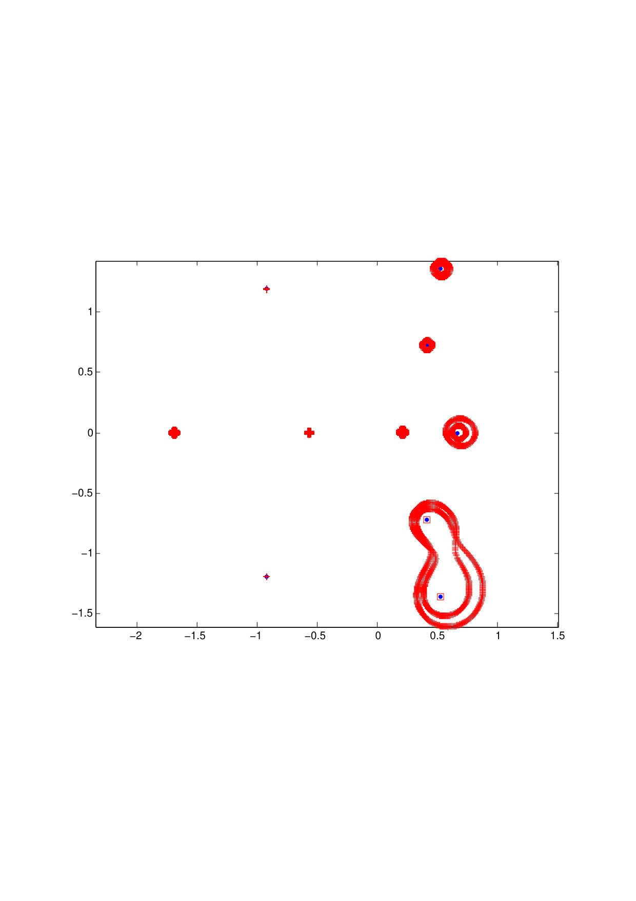 Figure 1
 Figure 2
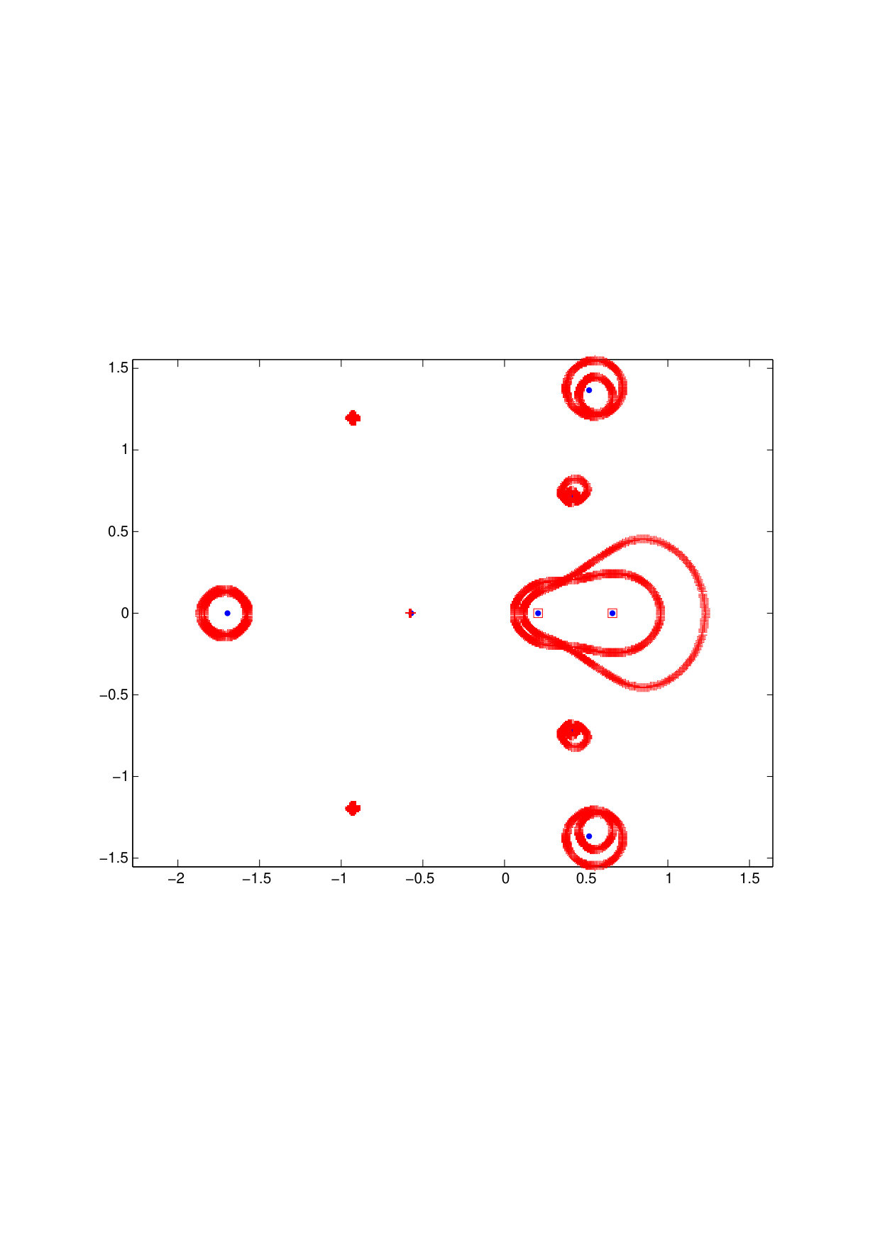 Figure 3
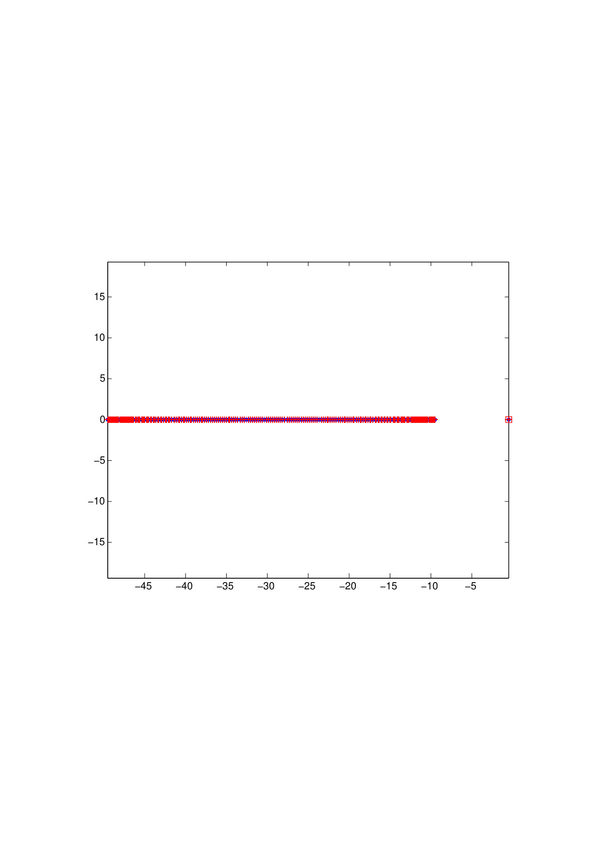 Figure 4
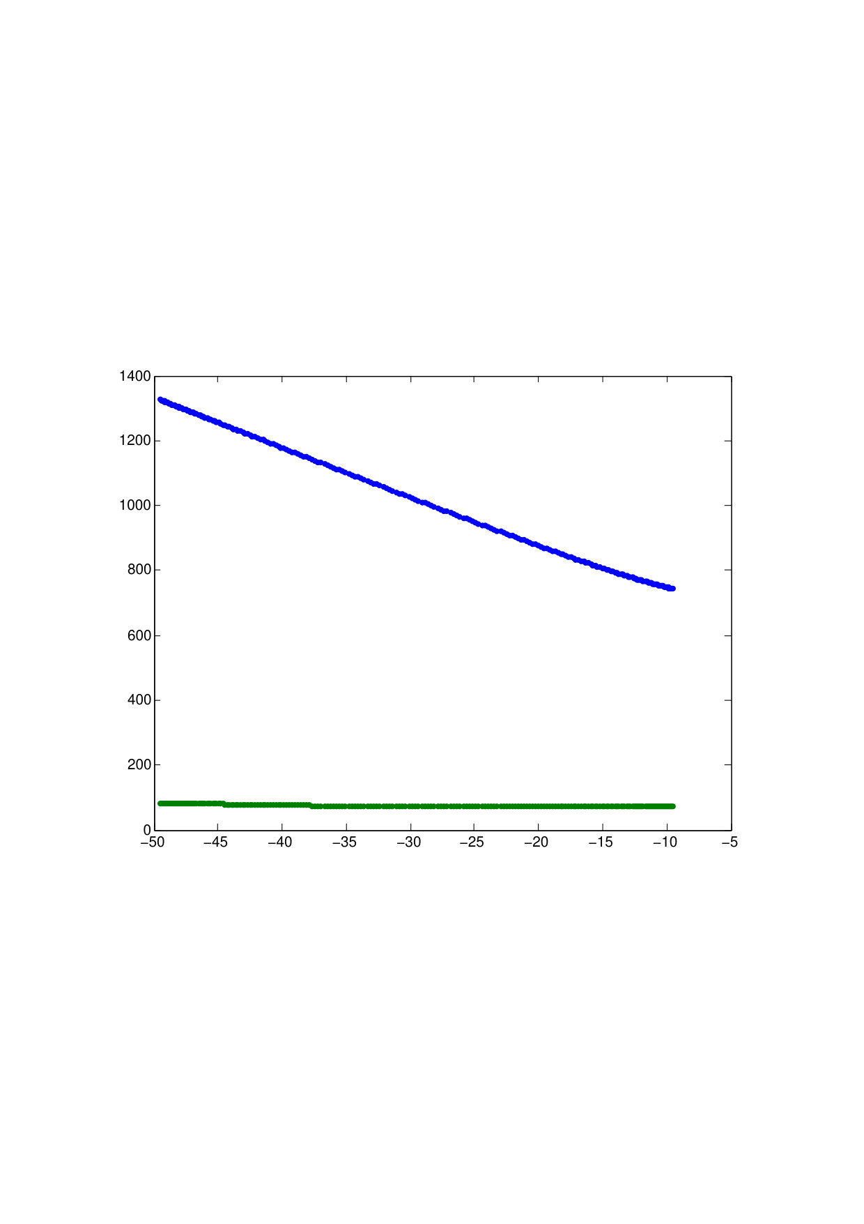 Figure 5
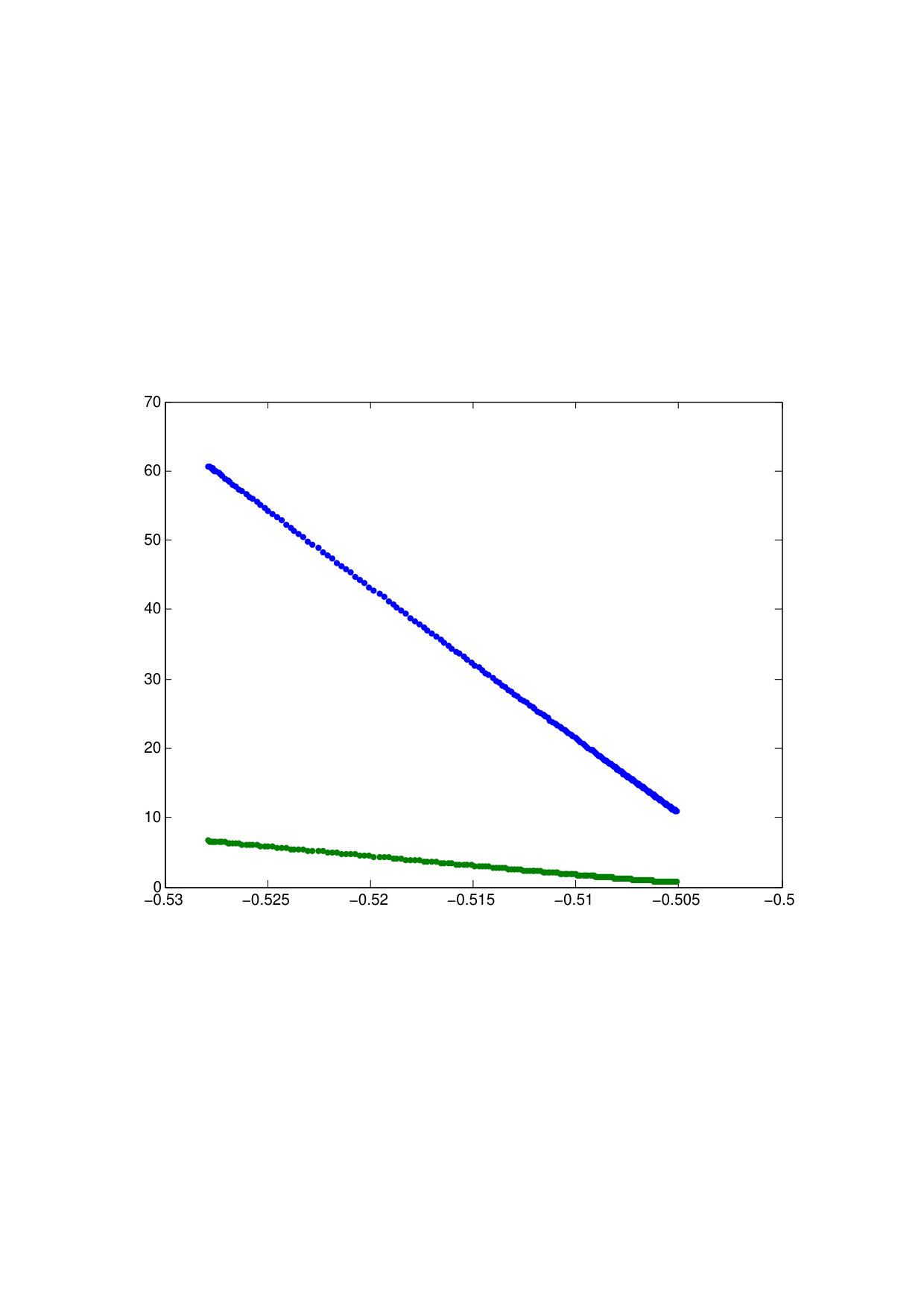 Figure 6
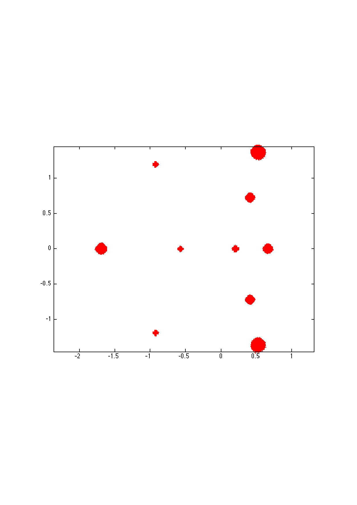 Figure 7
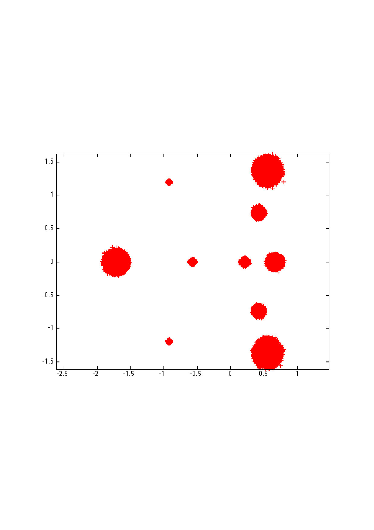 Figure 8
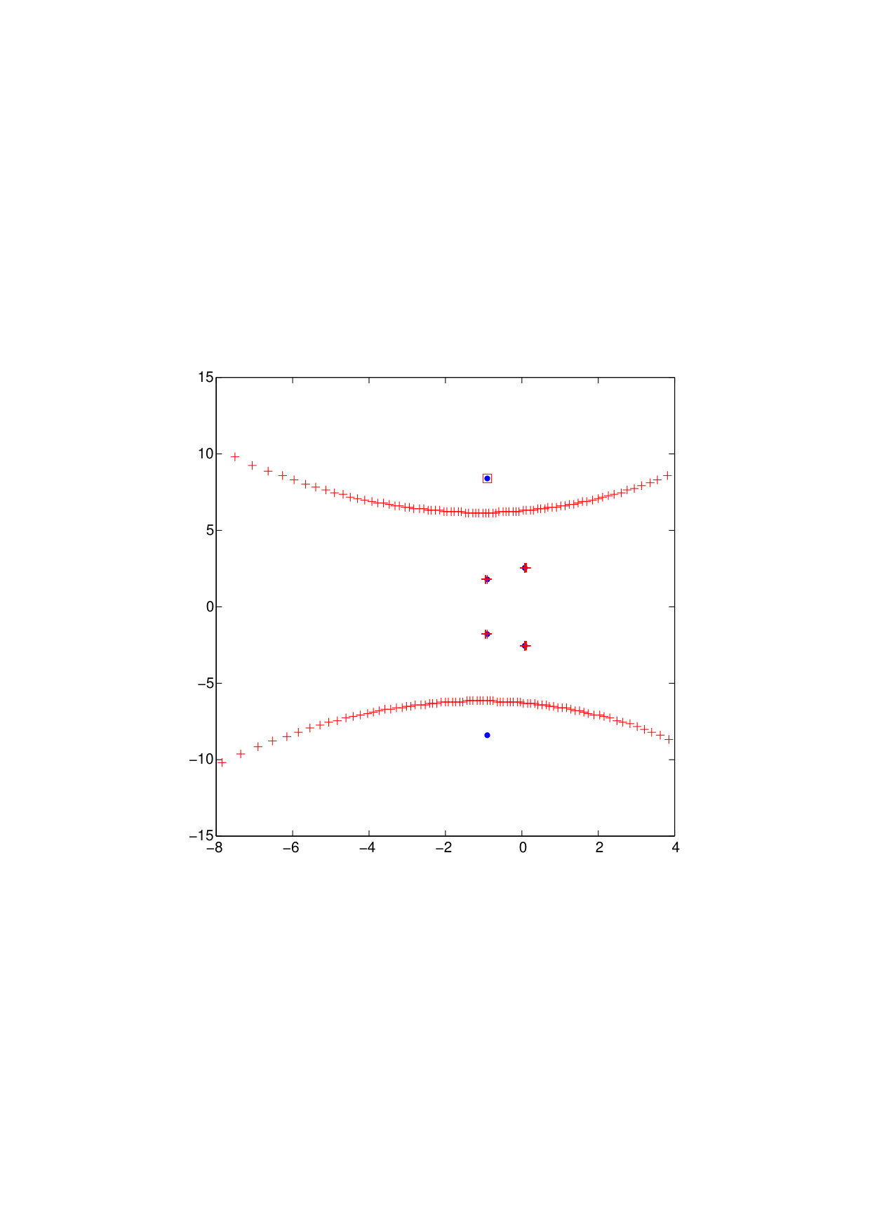 Figure 9
Peer Reviews
No public reviews on file for this paper yet. If you reviewed it on a platform where reviews are public (OpenReview, ICLR, NeurIPS, ICML), you can paste yours below so the community can read it here.
Videos
No videos yet. Explain this paper in a talk, walkthrough, or lecture? Add one.
\runningheads
S. Noschese and L. ReichelUnstructured and Structured Polynomial Pseudospectra
\corraddr
Dipartimento di Matematica, SAPIENZA Università di Roma, P.le Aldo Moro 5, 00185 Roma, Italy. E-mail: [email protected]. Work partially supported by INdAM-GNCS.
Computing Unstructured and Structured Polynomial Pseudospectrum Approximations
Silvia Noschese\corrauthand Lothar Reichel
1
2
11affiliationmark: Dipartimento di Matematica, SAPIENZA Università di Roma, P.le Aldo Moro 5, 00185 Roma, Italy.22affiliationmark: Department of Mathematical Sciences, Kent State University, Kent, OH 44242, USA.
Abstract
In many applications it is important to understand the sensitivity of eigenvalues of a matrix polynomial to perturbations of the polynomial. The sensitivity commonly is described by condition numbers or pseudospectra. However, the computation of pseudospectra of matrix polynomials is very demanding computationally. This paper describes a new approach to computing approximations of pseudospectra of matrix polynomials by using rank-one or projected rank-one perturbations. These perturbations are inspired by Wilkinson’s analysis of eigenvalue sensitivity. This approach allows the approximation of both structured and unstructured pseudospectra. Computed examples show the method to perform much better than a method based on random rank-one perturbations both for the approximation of structured and unstructured (i.e., standard) polynomial pseudospectra.
keywords:
matrix polynomials, pseudospectrum, structured pseudospectrum, eigenvalue sensitivity, distance from defectivity, numerical methods
1 Introduction
In many problems in science and engineering it is important to know the sensitivity of the eigenvalues of a square matrix to perturbations. The pseudospectrum is an important aid for shedding light on the sensitivity. Many properties and applications of the pseudospectrum of a matrix are discussed by Trefethen and Embree [23]; see also [6, 7, 10, 13, 20]. However, the computation of pseudospectra is a computationally demanding task except for very small matrices. Therefore, the development of numerical methods for the efficient computation of pseudospectra of medium-sized matrices, or partial pseudospectra of large matrices, has received considerable attention; see [3, 15, 18, 19, 25, 26].
The present paper is concerned with the computation of pseudospectra of matrix polynomials of the form
[TABLE]
where and , . We will assume that . Then has finite eigenvalues, i.e., there are no eigenvalues at infinity. Matrix polynomials of this kind arise in many applications in systems and control theory; see, e.g., [8, 9, 14]. The case corresponds to the generalized eigenvalue problem
[TABLE]
and the special case yields a standard eigenvalue problem. Here and throughout this paper denotes the identity matrix of order . In some applications the matrices in (1.1) have a structure that should be respected, such as being symmetric, skew-symmetric, banded, Toeplitz, or Hankel.
The sensitivity of the eigenvalues of a matrix polynomial (1.1) to perturbations in the matrices is important in applications. This question therefore has received considerable attention; see, e.g., [4, 10, 12, 21, 22] and references therein. When the matrices are structured, it is natural to only consider perturbations that are similarly structured.
Define the spectrum of ,
[TABLE]
Given a set of matrices , , and a set of weights , for all , we let the class of admissible perturbed matrix polynomials be
[TABLE]
The parameters , , determine the maximum norm of the perturbation of each matrix , where denotes the Frobenius norm. For instance, to keep unperturbed, we set .
One approach to investigate the sensitivity of the spectrum of a matrix polynomial to admissible perturbations is to compute and plot the -pseudospectrum of for several -values, where the -pseudospectrum of for is defined by
[TABLE]
The computation of a -pseudospectrum of a matrix polynomial generally is very computationally intensive, in fact, it is much more demanding than the computation of the -pseudospectrum of a single matrix; see Tisseur and Higham [22] for a discussion on several numerical methods including approaches based on using a transfer function, random perturbations, and projections to small-scale problems. The computations use the companion form of the matrix polynomial . This requires working with matrices of order , whose generalized Schur factorization is computed. Therefore, the computational methods can be expensive to apply when is fairly large and an approximation of the -pseudospectrum is determined on a mesh with many points. Details and counts of arithmetic floating point operations are provided in [22].
This paper describes a novel approach to approximate the -pseudospectra of by choosing particular rank-one perturbations of the matrices (or projected rank-one perturbations in case has a structure that is to be respected). The use of these rank-one perturbations yields approximations of the -pseudospectrum (1.3) for a lower computational cost than the computation of the -pseudospectrum. Our approach is inspired by Wilkinson’s analysis of eigenvalue perturbation of a single matrix; see [24]. It generalizes an approach recently developed in [18] for the efficient computation of structured or unstructured pseudospectra of a single matrix.
This paper is organized as follows. Section 2 reviews results on the sensitivity of a simple eigenvalue of a matrix polynomial, pseudospectra and the distance from defectivity for matrix polynomials is considered in Section 3, while the corresponding discussions for structured perturbations can be found in Sections 4 and 5. Algorithms for computing approximate structured and unstructured pseudospectra for matrix polynomials are described in Section 6, and a few computed examples are presented in Section 7. Finally, Section 8 contains concluding remarks.
2 The condition number of a simple eigenvalue of a matrix polynomial
Consider the matrix polynomial (1.1) and assume that the determinant of the leading coefficient matrix, , is nonvanishing. Let be an eigenvalue of . Then the linear system of equations P(\lambda_{0})\mbox{\boldmath{x}}=\mbox{\bf 0} has a nonzero solution \mbox{\boldmath{x}}_{0}\in\mathbb{C}^{n} (a right eigenvector), and there is a nonzero vector \mbox{\boldmath{y}}_{0}\in\mathbb{C}^{n} such that \mbox{\boldmath{y}}_{0}^{H}P(\lambda_{0})=\mbox{\bf 0}^{H} (left eigenvector). Here the superscript H denotes transposition and complex conjugation. The algebraic multiplicity of is its multiplicity as a zero of the scalar polynomial . The algebraic multiplicity is known to be larger than or equal to the geometric multiplicity of , which is the dimension of the null space of . The following result by Tisseur [21, Theorem 5] is important for the development of our numerical method. We therefore present a proof for completeness.
Proposition 2.1**.**
Let be a simple eigenvalue, i.e. , with corresponding right and left eigenvectors and of unit Euclidean norm. Here denotes the derivative of . Then the condition number of is given by
[TABLE]
where . The maximal perturbations are
[TABLE]
for any unimodular .
Proof.
Differentiating \sum_{j=0}^{m}(A_{j}+\epsilon\Delta_{j})\lambda^{j}(\varepsilon)\mbox{\boldmath{x}}(\varepsilon)=0 with respect to yields
[TABLE]
Setting , one obtains
[TABLE]
where . It follows that
[TABLE]
Applying \mbox{\boldmath{y}}^{H} to both the right-hand side and left-hand side of this equality yields
[TABLE]
where we note that \mbox{\boldmath{y}}^{H}P^{\prime}(\lambda)\mbox{\boldmath{x}}\neq 0 because is a simple eigenvalue; see [2, Theorem 3.2]. Observing that \mbox{\boldmath{y}}^{H}P(\lambda)=\mbox{\bf 0}^{H}, and dividing by \mbox{\boldmath{y}}^{H}P^{\prime}(\lambda)\mbox{\boldmath{x}}, one has
[TABLE]
Taking absolute values yields
[TABLE]
where the inequality follows from the bounds , . Finally, letting the matrix be a rank-one matrix of the form \eta\omega_{j}\mathrm{e}^{-\mathrm{i}j\arg(\lambda)}\mbox{\boldmath{y}}\mbox{\boldmath{x}}^{H} with unimodular (and therefore of Frobenius norm ) for all shows the proposition. ∎
Remark 2.2*.*
Consider the standard eigenvalue problem with , , and . Then and . Setting and , Proposition 2.1 yields the standard eigenvalue condition number \kappa(\lambda)=1/|\mbox{\boldmath{y}}^{H}\mbox{\boldmath{x}}|. When instead and , we obtain (and ), and the proposition gives the generalized eigenvalue condition number \kappa(\lambda)=(\omega_{0}+\omega_{1}|\lambda|)/|\mbox{\boldmath{y}}^{H}B\mbox{\boldmath{x}}|; see [11].
Remark 2.3*.*
If , the polynomial is scalar-valued. Let be a simple root of . Then the condition number of is .
3 The -pseudospectrum of a matrix polynomial and the distance from
defectivity
The -pseudospectrum of given by (1.3) is bounded if and only if for all such that . Therefore the boundedness of is guaranteed if is such that the origin does not belong to the -pseudospectrum of , which is given by
[TABLE]
It is easy to see that, if satisfies the constraint
[TABLE]
then a first order analysis suggests that no component of , which is approximately a disk of radius centered at for small enough, can contain the origin. The origin is on the border of the disk centered at when . Here denotes the traditional condition number of the eigenvalue of the matrix .
Since by assumption , the -pseudospectrum (1.3) has at most bounded connected components. Any small connected component of the -pseudospectrum that contains exactly one simple eigenvalue of the matrix polynomial is approximately a disk centered at with radius . A matrix polynomial is said to be defective if it has an eigenvalue , whose algebraic multiplicity is strictly larger than its geometric multiplicity; see [1]. Disjoint components of associated with distinct eigenvalues are, to a first order approximation, disjoint disks if is strictly smaller than the distance from defectivity of the matrix polynomial , where
[TABLE]
A rough estimate of is given by
[TABLE]
The disk centered at is tangential to the disk centered at when . Let the index pair minimize the ratio (3.1) over all distinct eigenvalue pairs. We will refer to the eigenvalues and as the most -sensitive pair of eigenvalues. We note that typically the most -sensitive pair of eigenvalues are not the eigenvalues with the largest condition numbers.
4 The structured condition number of a simple eigenvalue of a matrix polynomial
We briefly comment on structured eigenvalue condition numbers for a single matrix before turning to matrix polynomials. Consider the set of structured matrices. For instance, the set may consist of symmetric, tridiagonal, or Toeplitz matrices. We are concerned with structured perturbations in . Let denote the matrix in closest to with respect to the Frobenius norm. This projection is used in definition of the eigenvalue condition number for structured perturbations, see [5, 16, 17, 18], where it is shown that the eigenvalue condition number for structured perturbations is smaller than the eigenvalue condition number for unstructured perturbations. We also will use the normalized projection
[TABLE]
in the definition of maximal structured perturbations in Proposition 4.1 below.
Matrix polynomials (1.1) are defined by matrices , some or all of which may have a structure that is important for the application at hand. We refer to a matrix polynomial with at least one structured matrix as a structured matrix polynomial. To measure the sensitivity of the eigenvalues of a structured matrix polynomial to similarly structured perturbations, we proceed as follows. Let be a set of structured matrices that the matrix of the matrix polynomial belongs to. If has no particular structure, then . Introduce the set of sets of structured matrices and let the class of admissible perturbed matrix polynomials be
[TABLE]
Proposition 4.1**.**
Let be a simple eigenvalue with corresponding right and left eigenvectors and of unit Euclidean norm. Then the structured condition number of is given by
[TABLE]
where
[TABLE]
The maximal perturbations are given by
[TABLE]
for any unimodular .
Proof.
Differentiating \sum_{j=0}^{m}(A_{j}+\epsilon\Delta_{j})\lambda^{j}(\varepsilon)\mbox{\boldmath{x}}(\varepsilon)=\mbox{\bf 0} with respect to , as in the proof of Proposition 2.1, one obtains
[TABLE]
where satisfies , . Substituting , for , by the structured matrix \eta\omega_{j}\mbox{\boldmath{y}}\mbox{\boldmath{x}}^{H}|_{\widehat{{\mathcal{S}}}_{j}}\in{{\mathcal{S}}}_{j} with Frobenius norm , the upper bound \omega_{j}\,\|\mbox{\boldmath{y}}\mbox{\boldmath{x}}^{H}|_{{{\mathcal{S}}}_{j}}\|_{F} for |\mbox{\boldmath{y}}^{H}\Delta_{j}\mbox{\boldmath{x}}| is attained. Finally, letting \Delta_{j}=\eta\omega_{j}\mathrm{e}^{-\mathrm{i}j\arg(\lambda)}\mbox{\boldmath{y}}\mbox{\boldmath{x}}^{H}|_{\widehat{{\mathcal{S}}}_{j}} for all gives
[TABLE]
This concludes the proof. ∎
Remark 4.2*.*
The structured condition number (4.1) is bounded above by the (unstructured) condition number (2.1). In fact, the former can be much smaller than the latter. For instance, let us consider the quadratic eigenvalue problem P(\lambda)\mbox{\boldmath{x}}=\mathbf{0}, with \mbox{\boldmath{x}}\neq\mathbf{0}, where
[TABLE]
with the same structured mass matrix , damping matrix and stiffness matrix as in [22, Section 4.2], i.e., , , and . The eigenvalues of the polynomial matrix are real and negative. In more detail, the spectrum is split into two sets: eigenvalues are spread approximately uniformly in the interval and eigenvalues are clustered at . Figure 1 shows the unstructured (i.e., standard) condition numbers (top graph) and structured condiition numbers (bottom graph) for each eigenvalue. The unstructured condition numbers are seen to be much larger than the structured condition numbers.
5 The structured -pseudospectrum of a matrix polynomial and the
structured distance from defectivity
The -structured -pseudospectrum of is for defined by
[TABLE]
One has that is bounded if and only if for all such that . Thus, the boundedness of is guaranteed if is such that , where denotes the structured -pseudospectrum of , which is defined by
[TABLE]
We will assume that satisfies the constraint
[TABLE]
Then a first order analysis suggests that no component of contains the origin. In fact, when is small, the component that contains the eigenvalue of is approximately a disk of radius centered at . Here denotes the -structured condition number of the eigenvalue in , where belongs to the set of structured matrices in .
Any small connected component of that contains exactly one simple eigenvalue is approximately a disk centered at with radius . Such disks of for distinct eigenvalues are, to a first order approximation, disjoint if is strictly smaller than the structured distance from defectivity of the matrix polynomial . This distance is given by
[TABLE]
A rough estimate of is provided by
[TABLE]
Similarly as in Section 3, the disk centered at is tangential to the disk centered at when . Let the index pair minimize the ratio (5.2) over all distinct eigenvalue pairs. We will refer to the eigenvalues and as the most -sensitive pair of eigenvalues. We note that usually the most -sensitive pair of eigenvalues is not made up of the worst conditioned eigenvalues with respect to structured perturbations.
6 Algorithms
This section describes algorithms based on Propositions 2.1 and 4.1 for computing approximations of unstructured and structured pseudospectra of matrix polynomials.
Let \{\lambda_{i},\mbox{\boldmath{x}}_{i},\mbox{\boldmath{y}}_{i}\}_{i=1}^{mn} denote eigen-triplets made up of the eigenvalues and associated left and right unit eigenvectors, \mbox{\boldmath{x}}_{i} and \mbox{\boldmath{y}}_{i}, respectively, of the matrix polynomial defined by (1.1). We will assume the eigenvalues to be distinct. If a matrix polynomial has multiple eigenvalues, then we can apply the algorithms to the ones of algebraic multiplicity one. Throughout this section .
Algorithm 1 describes our numerical method for the approximation of the -pseudospectrum of a matrix polynomial defined by matrices , , without particular structure. The algorithm first determines an estimate of the distance to defectivity (3.1) of the matrix polynomial and the indices and of the most -sensitive pair of eigenvalues of . It then computes the rank-one matrices and defined in Proposition 2.1 for all (simple) eigenvalues of and for equidistant values on the unit circle in the complex plane. This defines the perturbations of the polynomial at the eigenvalues . The spectra of the perturbations of so obtained are displayed. This simple approach typically provides valuable insight into properties of the -pseudospectrum of .
Algorithm 2 is an analogue of Algorithm 1 for the approximation of the structured -pseudospectrum of a matrix polynomial. The algorithm differs from Algorithm 1 in that the distance to defectivity in the latter algorithm is replaced by the structured distance to defectivity (5.2) and the rank-one perturbations are replaced by structured rank-one perturbations defined in Proposition 4.1.
Both Algorithms 1 and 2 are easy to implement. The algorithms require the computation of the eigenvalues of polynomial matrices. Evaluating the spectrum of perturbed polynomial matrices is the main computational burden and easily can be implemented efficiently on a parallel computer. However, a laptop computer was sufficient for the computed examples reported in the following section.
7 Numerical examples
The computations were performed on a MacBook Air laptop computer with a 1.8Ghz CPU and 4 Gbytes of RAM. All computations were carried out in MATLAB with about significant decimal digits.
Example 1. Consider the matrix polynomial , where and are real matrices with normally distributed random entries with zero mean and variance, and is a real tridiagonal Toeplitz matrix of the same order with similarly distributed random diagonal, superdiagonal, and subdiagonal entries. We choose the weights , . The eigenvalues of and their standard and structured condition numbers are shown in Table 1. The structured condition numbers can be seen to be smaller than the standard condition numbers.
The estimate (3.1) of the (unstructured) distance from defectivity is . It is achieved for the indices and , as well as for the indices and , of the most -sensitive pairs of eigenvalues. The left plot in Figure 2 displays the spectrum of matrix polynomials of the form and for , , and . Thus, the spectrum of matrix polynomials are determined. Details of the computations are described by Algorithm 1. We recall that the “curves” surrounding the eigenvalues lie inside the -pseudospectrum of . The figure illustrates that the eigenvalues and might coalesce already for a small perturbation of .
We remark that since the matrices , , that define the matrix polynomial are real, the eigenvalues of appear in complex conjugate pairs. The pseudospectrum of matrix polynomials determined by real matrices is known to be symmetric with respect to the real axis in the complex plane. The fact that the left plot of Figure 2 is not symmetric with respect to the imaginary axis depends on that it only shows the spectra of the matrix polynomials and associated with the eigenvalues and of , but not of the polynomials and associated with the eigenvalues and . A plot of eigenvalues of all these polynomials is symmetric with respect to the real axis in the complex plane.
We compare the approximation of the -pseudospectrum shown in the left plot of Figure 2 with an approximation of the -pseudospectrum obtained by perturbing by random rank-one matrices. Specifically, the right plot of Figure 2 shows the spectrum of matrix polynomials of the form with , , where , and . Here is a rank-one random matrix scaled to have unit Frobenius norm. Despite using perturbations of , which are many more perturbations than used for producing the left plot, the right plot of Figure 2 does not indicate that any eigenvalue of might coalesce under small perturbations of the matrix polynomial. This important property clearly is difficult to detect by using random rank-one perturbations.
Next we turn to structured pseudospectra and perturbations. We obtain from (5.2) the estimate of the structured distance from defectivity . It is achieved for the eigenvalues and . The left plot in Figure 3 displays the spectra of matrix polynomials of the form and with , , for . The computations are described by Algorithm 2. The plot shows that the eigenvalues and might coalesce under small perturbations of .
The right plot of Figure 2 shows the spectrum of matrix polynomials of the form with , , where , , and is a unit-norm rank-one random matrix projected into . Despite using perturbations, the plot does not indicate that any eigenvalues of might coalesce under small structured perturbations.
Example 2. Consider the matrix polynomial defined by
[TABLE]
[TABLE]
This polynomial is discussed in [22, Section 4.1]. We choose similarly as in [22]. The eigenvalues and their condition numbers are shown in Table 2.
Figure 4 displays an approximation of the -pseudospectrum of obtained by letting (like in [22]) and computing the eigenvalues of matrix polynomials of the form for , , where is a maximal perturbation associated with the eigenvalue (marked by red square) with the largest condition number. Details of the computations are described by Algorithm 1.
Example 3. We consider the matrix polynomial with the structure defined in Remark 4.2. This polynomial is considered in [22, Section 4.2]. We choose the weights and obtain from (5.2) the estimate of the structured distance from defectivity . It is achieved for the eigenvalues and . These eigenvalues are the most -sensitive pair, but they are not the most ill-conditioned eigenvalues, despite that their relative distance is only .
Figure 5 displays the spectra of matrix polynomials of the form and with , . The computations are described by Algorithm 2.
8 Conclusions
This paper describes a novel and fairly inexpensive approach to determine the sensitivity of eigenvalues of a matrix polynomial. Eigenvalues of perturbed matrix polynomials are computed, where the perturbations are chosen to shed light on whether eigenvalues of the given matrix polynomial may coalesce under small perturbations.
The reference list from the paper itself. Each links out to its DOI / PubMed record.
- 1[1] Sk. S. Ahmad, R. Alam, and R. Byers, On pseudospectra, critical points, and multiple eigenvalues of matrix pencils, SIAM J. Matrix Anal. Appl., 31 (2010), pp. 1915–1933.
- 2[2] A. L. Andrew, K. W. E. Chu, and P. Lancaster, Derivatives of eigenvalues and eigenvectors of matrix functions, SIAM J. Matrix Anal. Appl., 14 (1993), pp. 903–926.
- 3[3] C. Bekas and E. Gallopoulos, Parallel computation of pseudospectra by fast descent, Parallel Computing, 28 (2002), pp. 223–242.
- 4[4] L. Boulton, P. Lancaster, and P. Psarrakos, On pseudospectra of matrix polynomials and their boundaries, Math. Comp., 77 (2008), pp. 313–334.
- 5[5] P. Buttà and S. Noschese, Structured maximal perturbations of Hamiltonian eigenvalue problems, J. Comput. Appl. Math., 272 (2014), pp. 304–312.
- 6[6] P. Buttà, N. Guglielmi, and S. Noschese, Computing the structured pseudospectrum of a Toeplitz matrix and its extremal points, SIAM J. Matrix Anal. Appl., 33 (2012), pp. 1300–1319.
- 7[7] P. Buttà, N. Guglielmi, M. Manetta, and S. Noschese, Differential equations for real-structured defectivity measures, SIAM J. Matrix Anal. Appl., 36 (2015), pp. 523–548.
- 8[8] I. Gohberg, P. Lancaster, and L. Rodman, Matrix Polynomials, SIAM, Philadelphia, 2009.