Thermal Feedback in the high-mass star and cluster forming region W51
Adam Ginsburg, Ciriaco Goddi, J.M. Diederik Kruijssen, John Bally,, Rowan Smith, Roberto Galv\'an-Madrid, Elisabeth A. C. Mills, Ke Wang, James, E. Dale, Jeremy Darling, Erik Rosolowsky, Robert Loughnane, Leonardo Testi,, Nate Bastian

TL;DR
This study uses ALMA observations to investigate the early stages of high-mass star formation in W51, revealing extended warm gas around protostars and providing insights into their accretion process before reaching the main sequence.
Contribution
It presents observational evidence of high gas temperatures around early-stage high-mass stars, challenging assumptions about their formation and accretion processes.
Findings
High temperatures (>100 K) extend to 5000 AU from protostars.
No signs of disks or rotation detected at 1000 AU resolution.
Early-stage protostars are not on the main sequence and may be bloated.
Abstract
High-mass stars have generally been assumed to accrete most of their mass while already contracted onto the main sequence, but this hypothesis has not been observationally tested. We present ALMA observations of a 3 x 1.5 pc area in the W51 high-mass star-forming complex. We identify dust continuum sources and measure the gas and dust temperature through both rotational diagram modeling of CH3OH and brightness-temperature-based limits. The observed region contains three high-mass YSOs that appear to be at the earliest stages of their formation, with no signs of ionizing radiation from their central sources. The data reveal high gas and dust temperatures (T > 100 K) extending out to about 5000 AU from each of these sources. There are no clear signs of disks or rotating structures down to our 1000 AU resolution. The extended warm gas provides evidence that, during the process of forming,…
Click any figure to enlarge with its caption.
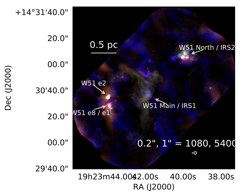 Figure 1
 Figure 2
 Figure 3
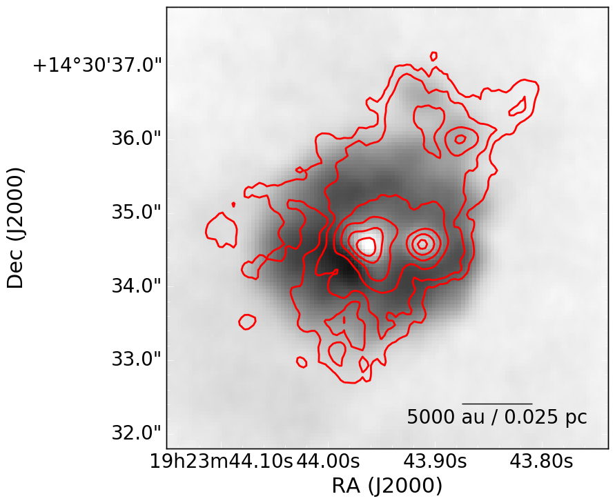 Figure 4
 Figure 5
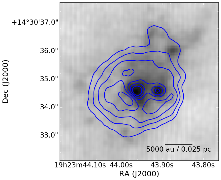 Figure 6
 Figure 7
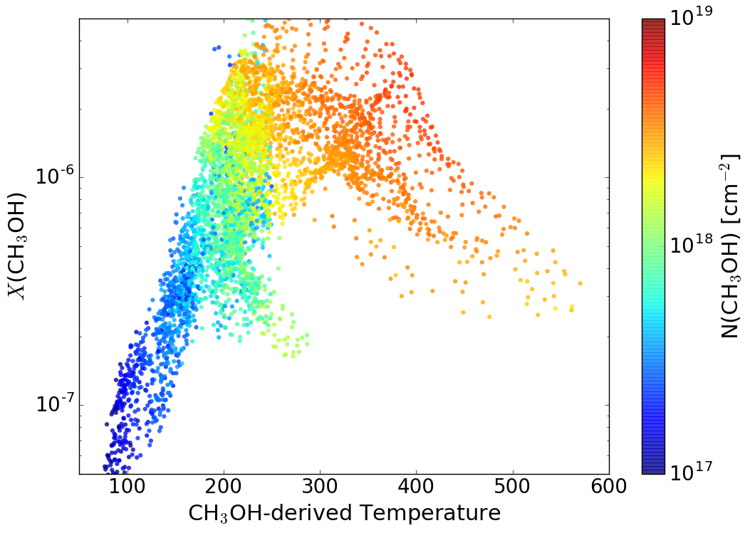 Figure 8
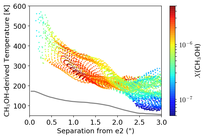 Figure 9
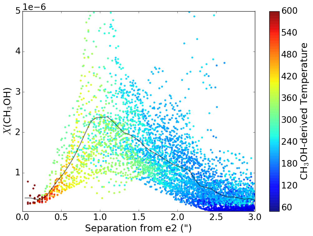 Figure 10
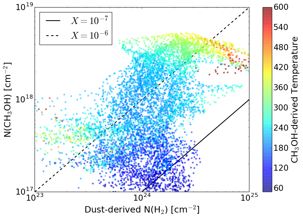 Figure 11
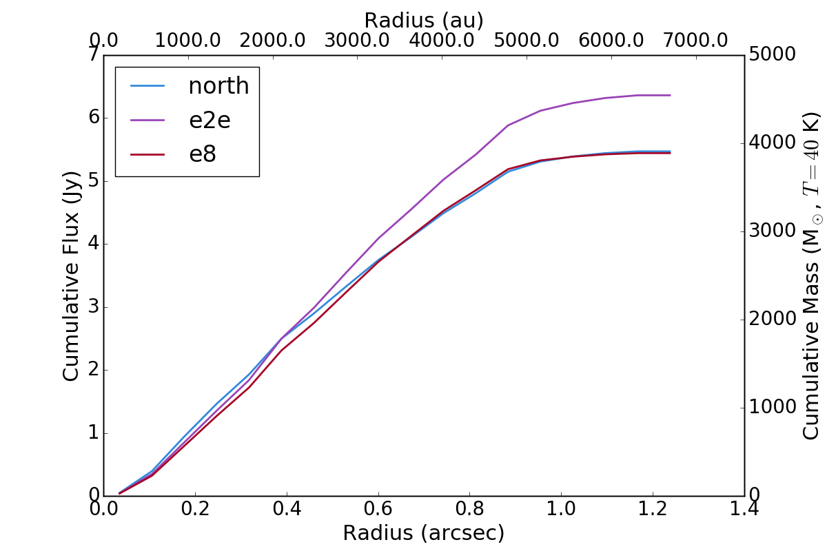 Figure 12
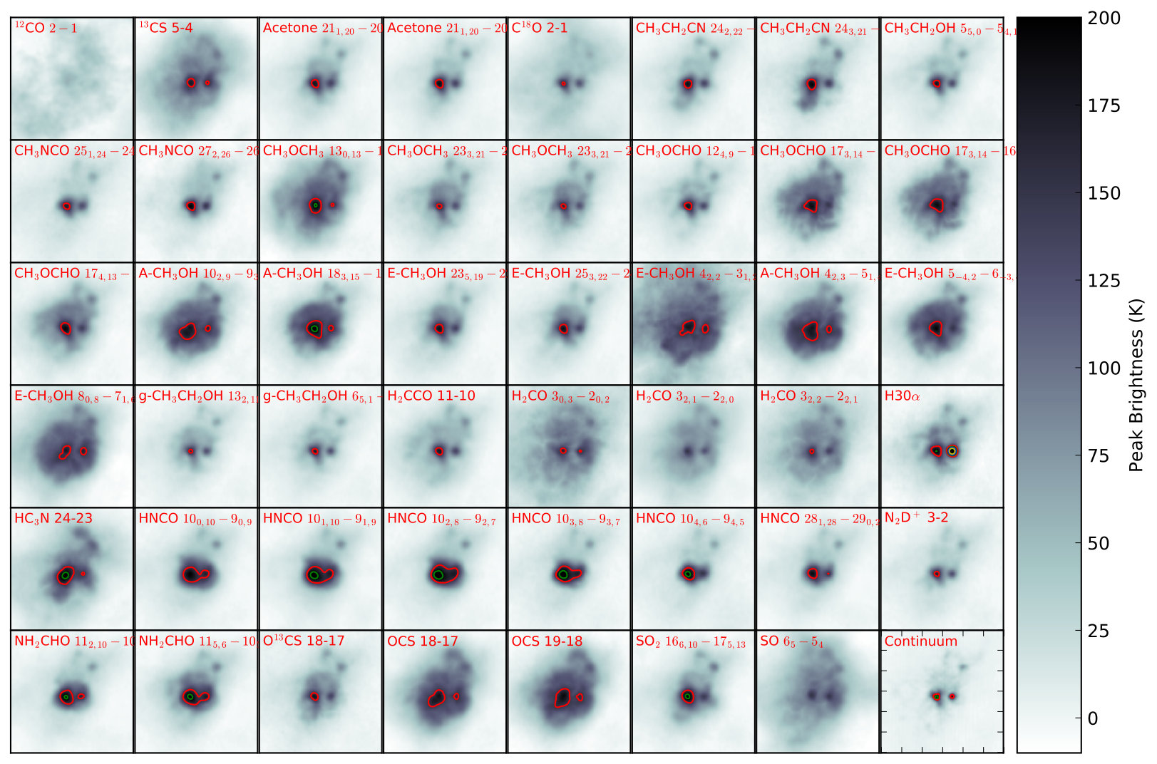 Figure 13
 Figure 14
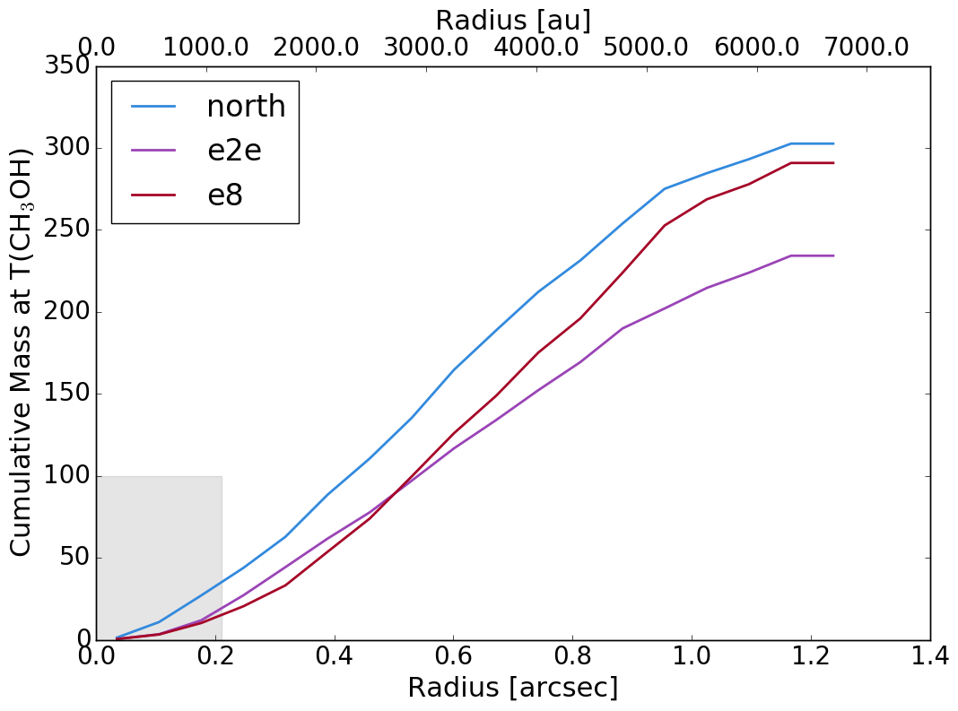 Figure 15
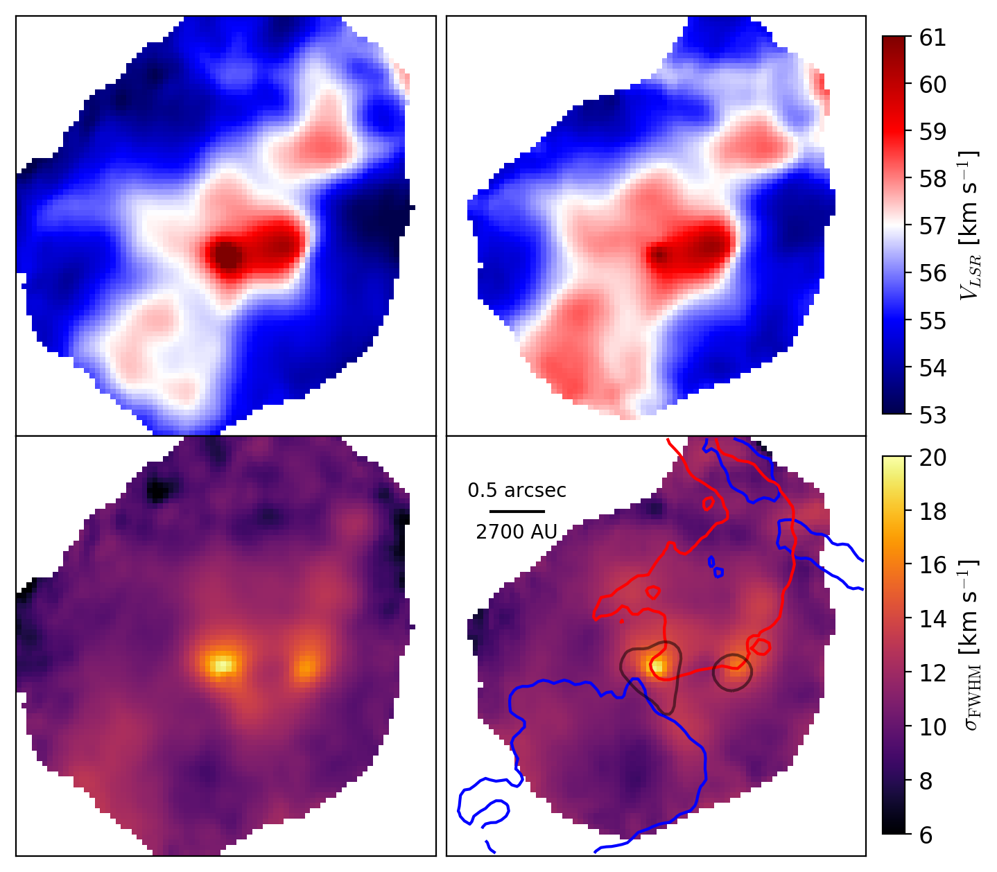 Figure 16
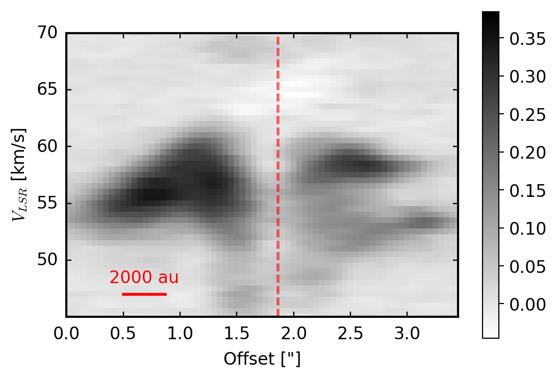 Figure 17
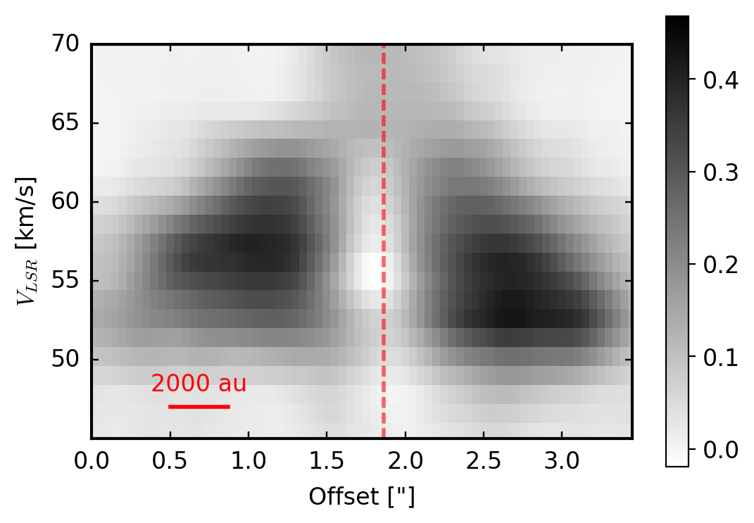 Figure 18
 Figure 19
 Figure 20
 Figure 21
 Figure 22
 Figure 23
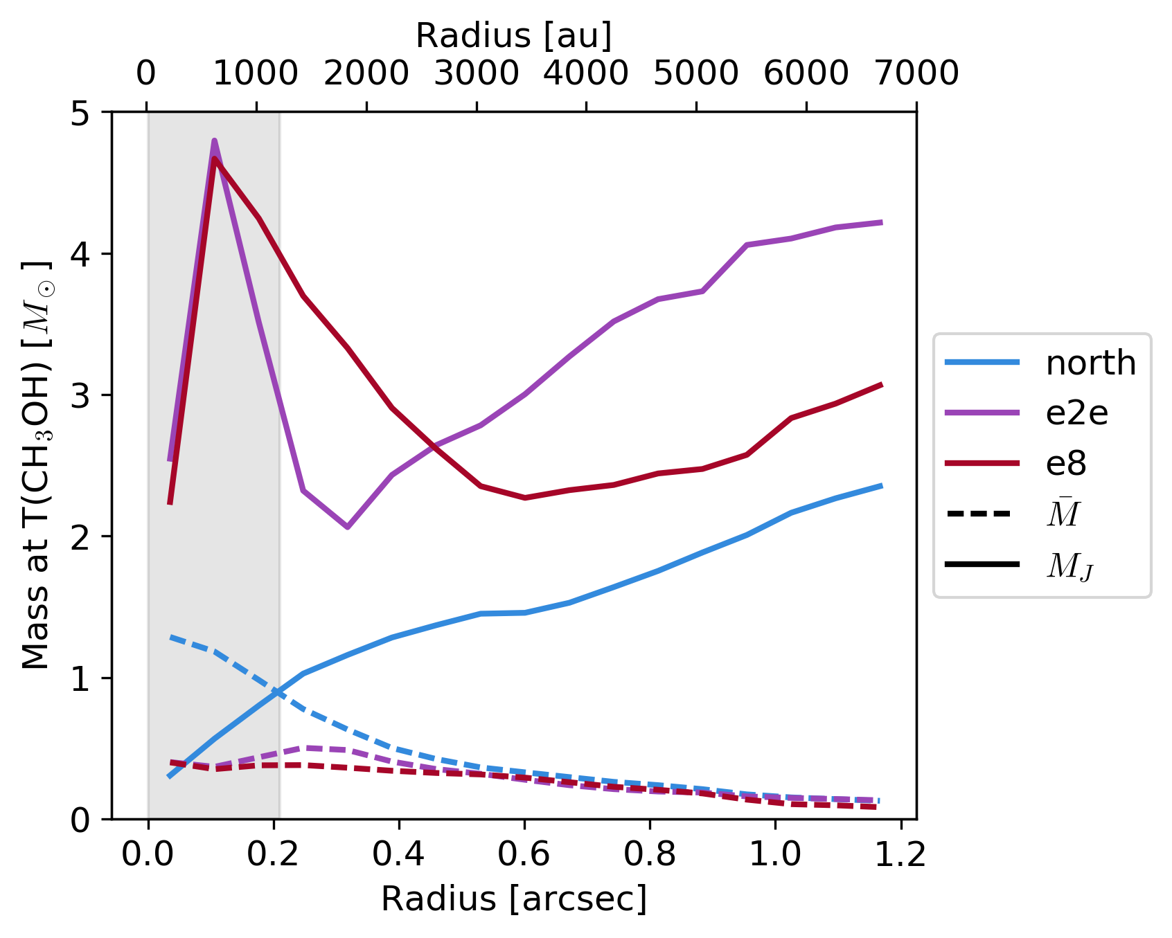 Figure 24
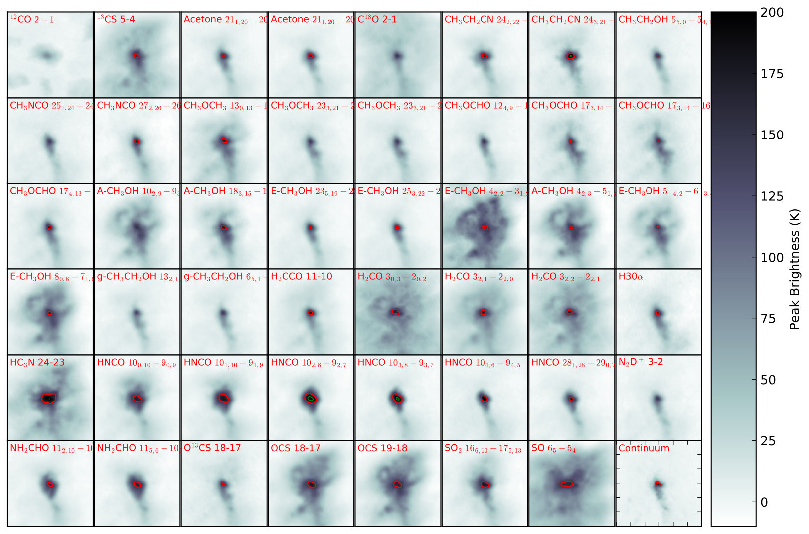 Figure 25
 Figure 26
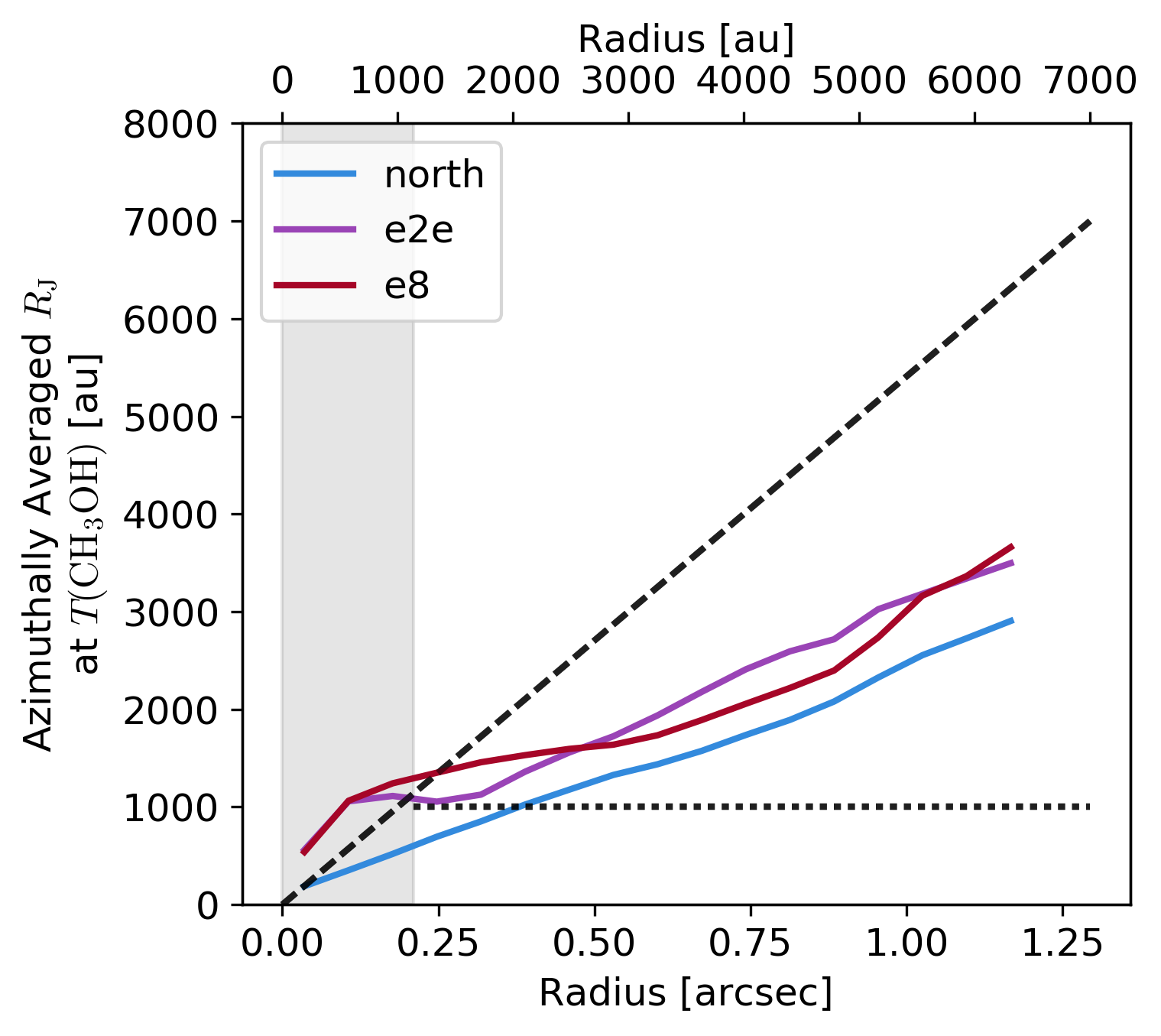 Figure 27
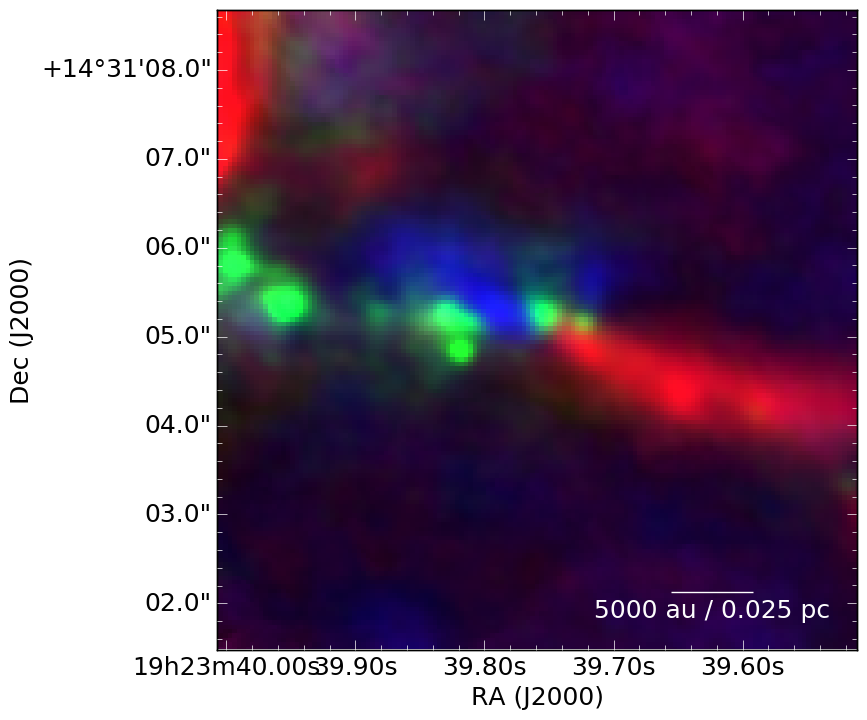 Figure 28
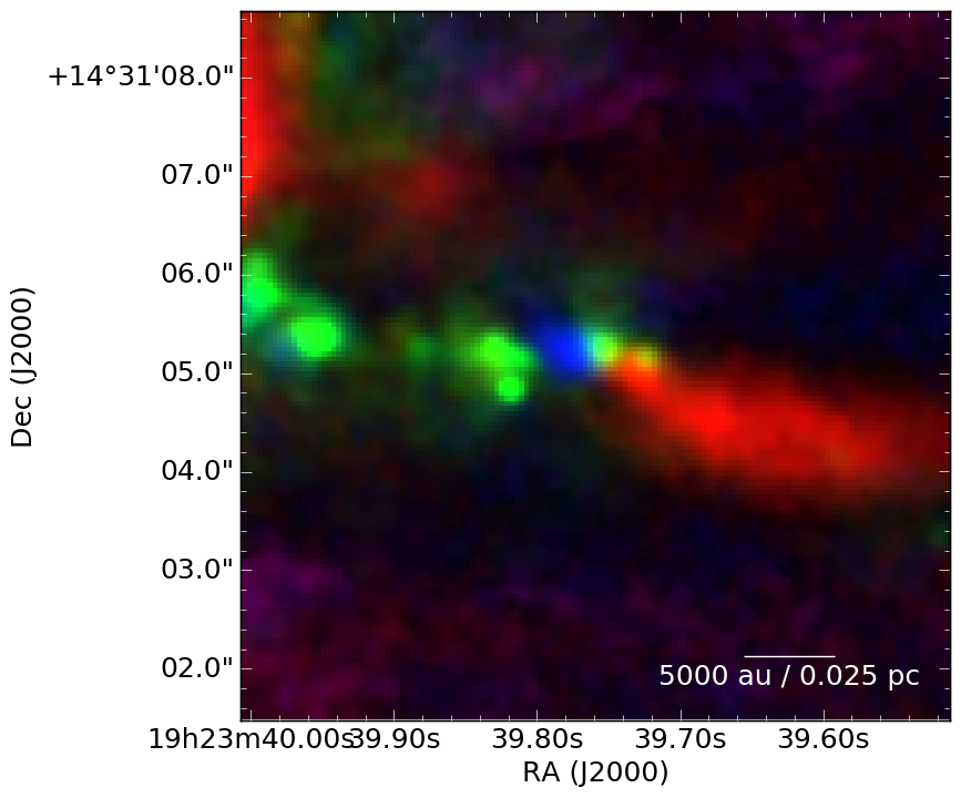 Figure 29
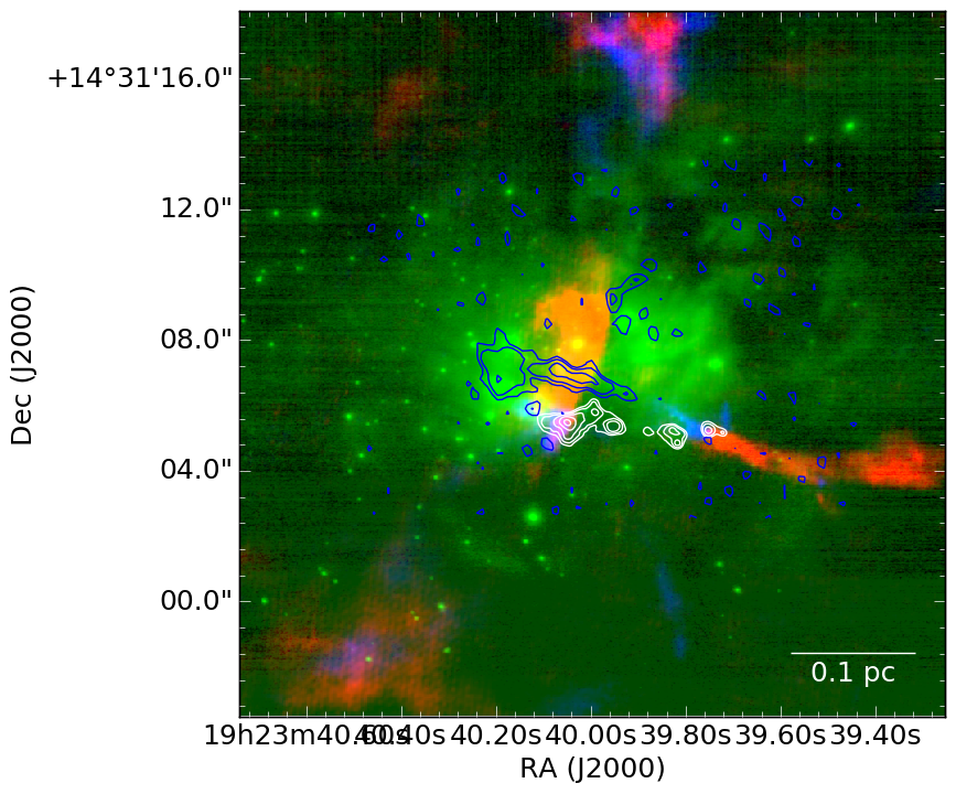 Figure 30
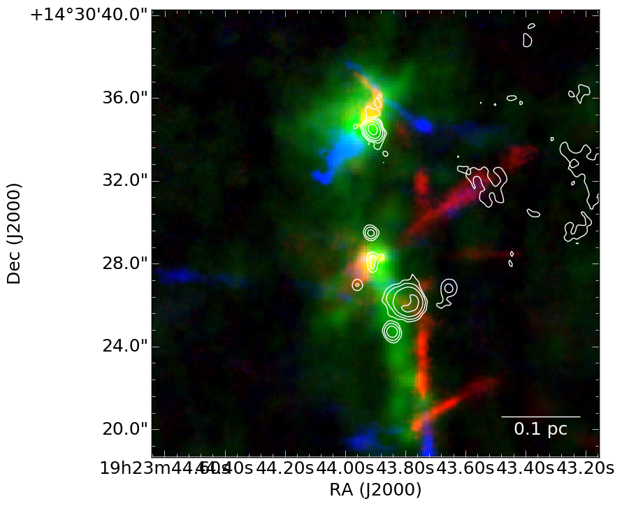 Figure 31
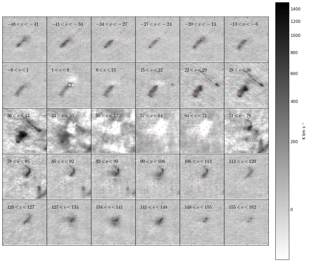 Figure 32
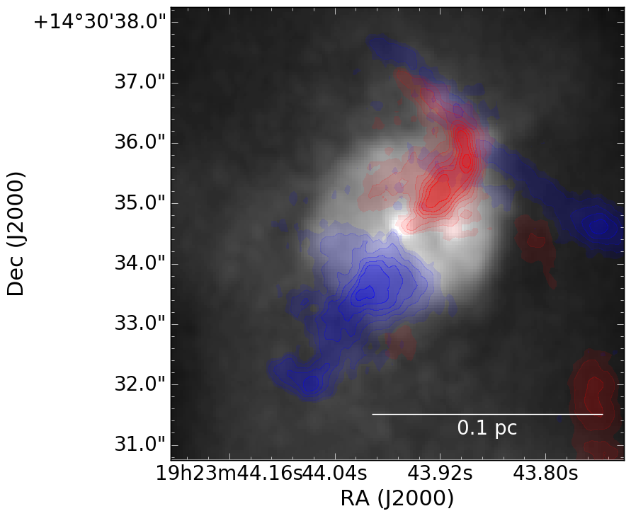 Figure 33
 Figure 34
 Figure 35
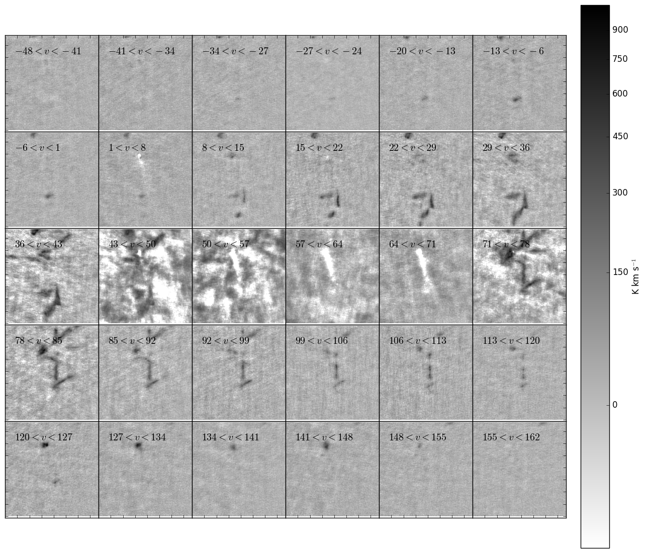 Figure 36
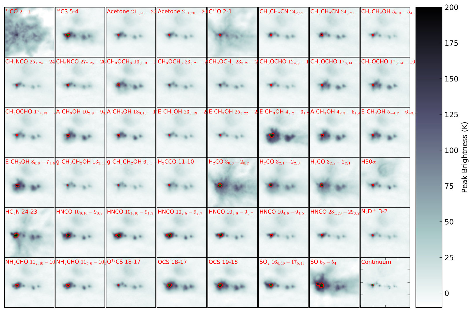 Figure 37
 Figure 38
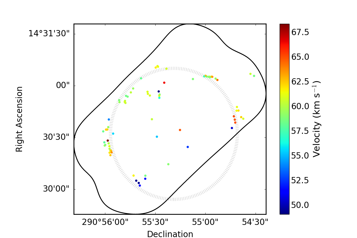 Figure 39
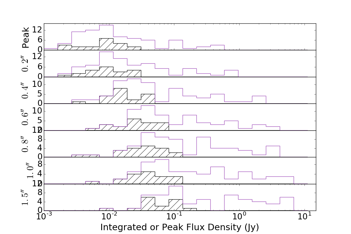 Figure 40
| SpwID | Minimum Frequency | Maximum Frequency | Channel Width [] | Channel Width [] |
|---|---|---|---|---|
| 0 | 218.11930228 | 218.619301 | -122.07 | 0.17 |
| 1 | 218.36288652 | 220.355073 | -488.281 | 0.67 |
| 2 | 230.376575 | 232.36876148 | 488.281 | 0.64 |
| 3 | 232.981075 | 234.97326148 | 488.281 | 0.63 |
| Line Name | Frequency | EU |
|---|---|---|
| E-CH3OH | 218.44005 | 45.45988 |
| A-CH3OH | 234.68345 | 60.9235 |
| E-CH3OH | 220.07849 | 96.61336 |
| E-CH3OH | 234.69847 | 122.72222 |
| A-CH3OH | 231.28115 | 165.34719 |
| A-CH3OH | 233.7958 | 446.58025 |
| E-CH3OH | 219.99394 | 775.89371 |
| E-CH3OH | 219.98399 | 802.17378 |
| Line Name | Frequency |
|---|---|
| H2CO | 218.22219 |
| H2CO | 218.47564 |
| E-CH3OH | 218.44005 |
| CH3OCHO E | 218.28083 |
| CH3OCHO A | 218.29787 |
| CH3CH2CN | 218.39002 |
| Acetone AE | 218.24017 |
| O13CS 18-17 | 218.19898 |
| CH3OCH3 AA | 218.49441 |
| CH3OCH3 EE | 218.49192 |
| CH3NCO | 218.5418 |
| CH3SH | 218.18612 |
| Line Name | Frequency |
|---|---|
| H2CO | 218.76007 |
| HC3N 24-23 | 218.32471 |
| HC3Nv7=1 24-23a | 219.17358 |
| HC3Nv7=1 24-23a | 218.86063 |
| HC3Nv7=2 24-23 | 219.67465 |
| OCS 18-17 | 218.90336 |
| SO | 219.94944 |
| HNCO | 218.98102 |
| HNCO | 219.73719 |
| HNCO | 219.79828 |
| HNCO | 219.39241 |
| HNCO | 219.54708 |
| HNCO | 219.65677 |
| E-CH3OH | 220.07849 |
| E-CH3OH | 219.98399 |
| E-CH3OH | 219.99394 |
| C18O 2-1 | 219.56036 |
| H2CCO 11-10 | 220.17742 |
| HCOOH | 219.09858 |
| CH3OCHO A | 220.19027 |
| CH3CH2CN | 219.50559 |
| Acetone AE | 219.21993 |
| Acetone EE | 219.24214 |
| Acetone EE | 218.63385 |
| HCO | 219.90849 |
| SO2 | 219.27594 |
| SO2 | 218.99583 |
| SO2 | 219.46555 |
| SO2 | 220.16524 |
| Line Name | Frequency |
|---|---|
| 12CO | 230.538 |
| OCS 19-18 | 231.06099 |
| HNCO | 231.873255 |
| A-CH3OH | 231.28115 |
| 13CS 5-4 | 231.22069 |
| NH2CHO | 232.27363 |
| H30 | 231.90093 |
| CH3OCHO E | 231.01908 |
| CH3CH2OH | 231.02517 |
| CH3OCH3 AA | 231.98772 |
| N2D+ 3-2 | 231.32183 |
| g-CH3CH2OH | 230.67255 |
| g-CH3CH2OH | 230.79351 |
| g-CH3CH2OH | 230.95379 |
| g-CH3CH2OH | 230.99138 |
| SO2 | 232.21031 |
| CH3SH | 231.75891 |
| CH3SH | 230.64608 |
| Line Name | Frequency |
|---|---|
| A-CH3OH | 234.68345 |
| E-CH3OH | 234.69847 |
| A-CH3OH | 233.7958 |
| 13CH3OH | 234.01158 |
| PN | 234.93569 |
| NH2CHO | 233.59451 |
| Acetone AE | 234.86136 |
| SO2 | 234.42159 |
| CH3NCO | 234.08812 |
| CH3SH | 234.19145 |
| Source ID | RA | Dec | M | M | Categories | |||
|---|---|---|---|---|---|---|---|---|
| ALMAmm1 | 19:23:42.864 | 14:30:07.92 | 3.7 | 6.9 | 11 | 2.6 | 2.6 | fCc |
| ALMAmm2 | 19:23:42.394 | 14:30:07.86 | 4.2 | 7.3 | 4 | 3 | 12 | fCc |
| ALMAmm3 | 19:23:42.398 | 14:30:06.08 | 4.2 | 11 | nan | 3 | 2.9 | f– |
| ALMAmm4 | 19:23:42.614 | 14:30:02.14 | 7.7 | 16 | 11 | 5.4 | 6.1 | -Cc |
| ALMAmm5 | 19:23:42.658 | 14:30:03.63 | 1 | 19 | 5.9 | 7.3 | 8.8 | -Cc |
| ALMAmm6 | 19:23:42.758 | 14:30:04.97 | 2.8 | 9.2 | 3.8 | 2 | 1.1 | fC- |
| ALMAmm7 | 19:23:40.702 | 14:30:24.5 | 3.5 | 7.4 | 1.4 | 2.5 | 7.1 | -Cc |
| ALMAmm9 | 19:23:41.481 | 14:30:14.6 | 21 | 46 | 5.8 | 15 | 9 | -Cc |
| ALMAmm10 | 19:23:38.738 | 14:30:47.66 | 3.6 | 7.8 | 5.3 | 2.6 | 1 | -Cc |
| ALMAmm11 | 19:23:38.684 | 14:30:45.57 | 19 | 36 | 12 | 14 | 12 | -Cc |
| ALMAmm12 | 19:23:38.755 | 14:30:45.54 | 5.2 | 2 | 11 | 3.7 | 11 | -C- |
| ALMAmm13 | 19:23:38.825 | 14:30:40.31 | 7 | 12 | 11 | 5 | 8.6 | -Cc |
| ALMAmm14 | 19:23:38.57 | 14:30:41.79 | 67 | 14 | 36 | 23 | 23 | –c |
| ALMAmm15 | 19:23:38.486 | 14:30:40.86 | 14 | 31 | 35 | 4.9 | 8.1 | –c |
| ALMAmm16 | 19:23:38.2 | 14:31:06.85 | 23 | 45 | 5.6 | 16 | 32 | -Cc |
| ALMAmm17 | 19:23:42.214 | 14:30:54.31 | 15 | 26 | 12 | 11 | 5 | fCc |
| ALMAmm18 | 19:23:42.293 | 14:30:55.29 | 15 | 31 | 5.6 | 11 | 4.1 | -Cc |
| ALMAmm19 | 19:23:42.307 | 14:30:56.49 | 4.9 | 13 | 21 | 3.2 | 1.4 | — |
| ALMAmm20 | 19:23:41.64 | 14:31:01.75 | 8 | 21 | 6.6 | 5.7 | 4 | -C- |
| ALMAmm21 | 19:23:41.981 | 14:31:10.52 | 8.9 | 15 | nan | 6.3 | 31 | –c |
| ALMAmm22 | 19:23:41.909 | 14:31:11.38 | 8.6 | 23 | nan | 6.1 | 18 | — |
| ALMAmm23 | 19:23:40.496 | 14:31:03.94 | 22 | 65 | 26 | 11 | 5.2 | — |
| ALMAmm24 | 19:23:39.953 | 14:31:05.35 | 29 | 6 | 72 | 46 | 32 | -Hc |
| ALMAmm25 | 19:23:42.132 | 14:30:40.57 | 18 | 38 | 3.8 | 13 | 6 | fCc |
| ALMAmm26 | 19:23:43.102 | 14:30:53.66 | 13 | 32 | 8.9 | 9.5 | 14 | -Cc |
| ALMAmm27 | 19:23:42.967 | 14:30:56.18 | 1 | 27 | 5 | 7.2 | 8.2 | fC- |
| ALMAmm28 | 19:23:43.68 | 14:30:32.24 | 16 | 33 | 19 | 11 | 6.5 | -Cc |
| ALMAmm29 | 19:23:41.933 | 14:30:30.45 | 9 | 16 | nan | 6.4 | 11 | f-c |
| ALMAmm30 | 19:23:43.164 | 14:30:54.12 | 8.3 | 2 | 4.3 | 5.9 | 2 | fCc |
| ALMAmm31 | 19:23:39.754 | 14:31:05.24 | 17 | 36 | 46 | 43 | 16 | –c |
| ALMAmm32 | 19:23:39.724 | 14:31:05.15 | 87 | 23 | 94 | 1 | 13 | -H- |
| ALMAmm33 | 19:23:39.828 | 14:31:05.23 | 19 | 51 | 48 | 48 | 18 | — |
| ALMAmm34 | 19:23:39.878 | 14:31:05.19 | 8 | 24 | 9 | 1 | 1 | -H- |
| ALMAmm35 | 19:23:39.991 | 14:31:05.77 | 2 | 58 | 34 | 76 | 18 | — |
| ALMAmm36 | 19:23:39.518 | 14:31:03.33 | 22 | 47 | 11 | 16 | 6.5 | -Cc |
| Source ID | RA | Dec | M | M | Categories | |||
| ALMAmm37 | 19:23:41.825 | 14:30:54.9 | 17 | 36 | 34 | 6.4 | 3.1 | –c |
| ALMAmm38 | 19:23:41.011 | 14:30:34.34 | 2.4 | 4.8 | 2 | 1.7 | 15 | -Cc |
| ALMAmm39 | 19:23:41.887 | 14:31:11 | 7.7 | 22 | 3.4 | 5.5 | 25 | -C- |
| ALMAmm40 | 19:23:41.549 | 14:31:09.87 | 7.5 | 18 | 9.2 | 5.3 | 5.5 | -Cc |
| ALMAmm41 | 19:23:43.85 | 14:30:40.43 | 2 | 29 | 3 | 8.6 | 13 | –c |
| ALMAmm43 | 19:23:39.59 | 14:31:04.13 | 19 | 53 | 17 | 14 | 4.8 | fC- |
| ALMAmm44 | 19:23:38.054 | 14:31:05.68 | 8.4 | 19 | 5.7 | 6 | 28 | -Cc |
| ALMAmm45 | 19:23:38.76 | 14:31:07.22 | 7.3 | 2 | 4.4 | 5.2 | 1.8 | -C- |
| ALMAmm46 | 19:23:41.834 | 14:30:52.99 | 15 | 37 | 24 | 8.5 | 3 | — |
| ALMAmm47 | 19:23:42.569 | 14:31:04.27 | 6.3 | 14 | 4.9 | 4.5 | 9.2 | -Cc |
| ALMAmm48 | 19:23:42.881 | 14:30:58.4 | 9.4 | 19 | 8.1 | 6.7 | 13 | -Cc |
| ALMAmm49 | 19:23:43.205 | 14:30:51.2 | 15 | 46 | 21 | 9.8 | 7.6 | — |
| ALMAmm50 | 19:23:43.217 | 14:30:50.6 | 2 | 53 | 14 | 14 | 6.3 | -C- |
| ALMAmm51 | 19:23:43.188 | 14:30:50.01 | 19 | 46 | 16 | 13 | 2.7 | -C- |
| ALMAmm52 | 19:23:38.806 | 14:30:38.62 | 4.9 | 9.7 | 7.9 | 3.5 | 1 | -Cc |
| ALMAmm53 | 19:23:38.861 | 14:30:42.25 | 8 | 18 | 13 | 5.7 | 5.6 | -Cc |
| ALMAmm54 | 19:23:38.94 | 14:30:35.48 | 5.1 | 9.7 | 2.5 | 3.6 | 9.7 | -Cc |
| ALMAmm55 | 19:23:43.426 | 14:30:50.46 | 11 | 29 | 4.5 | 7.7 | 6.5 | -C- |
| ALMAmm56 | 19:23:43.44 | 14:30:51.61 | 9 | 25 | 5.3 | 6.4 | 5.4 | -C- |
| ALMAmm57 | 19:23:41.731 | 14:30:52.99 | 5.6 | 1 | 2 | 4 | 1.2 | fCc |
| d2 | 19:23:39.818 | 14:31:04.83 | 16 | 43 | 99 | 18 | 15 | -H- |
| e1mm1 | 19:23:43.86 | 14:30:26.58 | 16 | 42 | 23 | 95 | 31 | — |
| e2e | 19:23:43.956 | 14:30:34.57 | 69 | 19 | 84 | 94 | 61 | -H- |
| e2e peak | 19:23:43.963 | 14:30:34.56 | 74 | 18 | 1 | 8 | 68 | -Hc |
| e2nw | 19:23:43.874 | 14:30:35.99 | 22 | 51 | 4 | 69 | 33 | –c |
| e2se | 19:23:44.076 | 14:30:33.53 | 36 | 98 | 93 | 4.4 | 7.3 | -H- |
| e2w | 19:23:43.91 | 14:30:34.61 | 54 | 12 | 85 | 72 | 6 | fHc |
| e3mm1 | 19:23:43.829 | 14:30:24.95 | 5 | 18 | 23 | 29 | 9.4 | — |
| e5 | 19:23:41.862 | 14:30:56.69 | 25 | 31 | nan | 18 | 34 | F-c |
| e8mm | 19:23:43.894 | 14:30:28.2 | 68 | 17 | 18 | 43 | 16 | -H- |
| eEmm1 | 19:23:44.016 | 14:30:25.32 | 38 | 1 | 39 | 12 | 7 | — |
| eEmm2 | 19:23:43.994 | 14:30:25.7 | 37 | 1 | 22 | 24 | 6.5 | — |
| eEmm3 | 19:23:44.03 | 14:30:27.17 | 43 | 95 | 22 | 27 | 8.1 | –c |
| eSmm1 | 19:23:43.822 | 14:30:23.44 | 69 | 18 | 34 | 26 | 2 | — |
| eSmm2 | 19:23:43.788 | 14:30:22.42 | 68 | 17 | 29 | 31 | 23 | –c |
| eSmm2a | 19:23:43.764 | 14:30:22.38 | 5 | 13 | 24 | 28 | 18 | — |
| eSmm3 | 19:23:43.74 | 14:30:21.37 | 52 | 99 | 29 | 23 | 16 | –c |
| eSmm4 | 19:23:43.822 | 14:30:21.18 | 36 | 96 | 27 | 17 | 1 | — |
| eSmm6 | 19:23:43.788 | 14:30:19.74 | 5 | 11 | 23 | 29 | 15 | –c |
| north | 19:23:40.044 | 14:31:05.42 | 72 | 17 | 69 | 12 | 59 | -Hc |
Peer Reviews
No public reviews on file for this paper yet. If you reviewed it on a platform where reviews are public (OpenReview, ICLR, NeurIPS, ICML), you can paste yours below so the community can read it here.
Videos
No videos yet. Explain this paper in a talk, walkthrough, or lecture? Add one.
Thermal Feedback in the high-mass star and cluster forming region W51
*Jansky fellow of the National Radio Astronomy Observatory, Socorro, NM 87801 USA *
- European Southern Observatory, Karl-Schwarzschild-Straße 2, D-85748 Garching bei München, Germany *
Ciriaco Goddi
Department of Astrophysics/IMAPP, Radboud University Nijmegen, PO Box 9010, 6500 GL Nijmegen, the Netherlands
ALLEGRO/Leiden Observatory, Leiden University, PO Box 9513, 2300 RA Leiden, the Netherlands
J. M. Diederik Kruijssen
Astronomisches Rechen-Institut, Zentrum für Astronomie der Universität Heidelberg, Mönchhofstraße 12-14, 69120 Heidelberg, Germany
John Bally
CASA, University of Colorado, 389-UCB, Boulder, CO 80309
Rowan Smith
Jodrell Bank Centre for Astrophysics, School of Physics and Astronomy, University of Manchester, Oxford Road, Manchester M13 9PL, UK
Roberto Galván-Madrid
Instituto de Radioastronomía y Astrofísica, UNAM, A.P. 3-72, Xangari, Morelia, 58089, Mexico
Elisabeth A.C. Mills
San Jose State University, One Washington Square, San Jose, CA 95192
Ke Wang
- European Southern Observatory, Karl-Schwarzschild-Straße 2, D-85748 Garching bei München, Germany *
James E. Dale
Centre for Astrophysics Research, University of Hertfordshire, College Lane, Hatfield, AL10 9AB, UK
Jeremy Darling
CASA, University of Colorado, 389-UCB, Boulder, CO 80309
Erik Rosolowsky
Dept. of Physics, University of Alberta, Edmonton, Alberta, Canada
Robert Loughnane
Instituto de Radioastronomía y Astrofísica, UNAM, A.P. 3-72, Xangari, Morelia, 58089, Mexico
Leonardo Testi
- European Southern Observatory, Karl-Schwarzschild-Straße 2, D-85748 Garching bei München, Germany *
*INAF-Osservatorio Astrofisico di Arcetri, Largo E. Fermi 5, I-50125, Florence, Italy *
*Excellence Cluster Universe, Boltzman str. 2, D-85748 Garching bei München, Germany *
Nate Bastian
*Astrophysics Research Institute, Liverpool John Moores University, 146 Brownlow Hill, Liverpool L3 5RF, UK * Adam Ginsburg [email protected]; [email protected]
Abstract
High-mass stars have generally been assumed to accrete most of their mass while already contracted onto the main sequence, but this hypothesis has not been observationally tested. We present ALMA observations of a pc area in the W51 high-mass star-forming complex. We identify dust continuum sources and measure the gas and dust temperature through both rotational diagram modeling of and brightness-temperature-based limits. The observed region contains three high-mass YSOs that appear to be at the earliest stages of their formation, with no signs of ionizing radiation from their central sources. The data reveal high gas and dust temperatures ( K) extending out to about 5000 AU from each of these sources. There are no clear signs of disks or rotating structures down to our 1000 AU resolution. The extended warm gas provides evidence that, during the process of forming, these high-mass stars heat a large volume and correspondingly large mass of gas in their surroundings, inhibiting fragmentation and therefore keeping a large reservoir available to feed from. By contrast, the more mature massive stars that illuminate compact H ii regions have little effect on their surrounding dense gas, suggesting that these main sequence stars have completed most or all of their accretion. The high luminosity of the massive protostars ( ), combined with a lack of centimeter continuum emission from these sources, implies that they are not on the main sequence while they accrete the majority of their mass; instead, they may be bloated and cool.
stars: massive, stars: formation, ISM: abundances, (ISM:) HII regions, ISM: individual objects (W51), ISM: molecules, submillimeter: ISM, radio continuum: ISM, radio lines: ISM
††facilities: ALMA, JVLA††software: astropy (Astropy Collaboration et al., 2013) ipython (Pérez & Granger, 2007) CASA https://casa.nrao.edu/ pyspeckit http://pyspeckit.bitbucket.org Ginsburg & Mirocha (2011) aplpy https://aplpy.github.io/ wcsaxes http://wcsaxes.readthedocs.org pvextractor http://pvextractor.readthedocs.org spectral cube http://spectral-cube.readthedocs.org ds9 http://ds9.si.edu dust_emissivity http://dust_emissivity.readthedocs.org
\savesymbol
doublespace
1 Introduction
High-mass stars are the drivers of galaxy evolution, cycling enriched materials into the interstellar medium (ISM) and illuminating it. During their formation process, however, these stars are nearly undetectable because of their rarity and their opaque surroundings. We therefore know relatively little about how massive stars acquire their mass and what their immediate surroundings look like at this early time. We expect, though, that the physical conditions should be changing rapidly.
The stellar initial mass function (IMF) appears to be a universal distribution (Bastian et al., 2010). However, massive O-stars (with ) almost always form in a clustered fashion (in proto-clusters or proto-associations; de Wit et al., 2004, 2005; Parker & Goodwin, 2007). Their presence, and the strong feedback they produce, may directly influence how the IMF around them is formed. If feedback from these stars is relevant while most of the mass surrounding them is still in gas (not yet in stars), the mass function in such clusters cannot be determined by ISM properties (initial conditions) alone.
Models of high-mass star formation universally have difficulty collapsing enough material to a stellar radius to form very massive stars. Generally, these models produce a high-mass star with enough luminosity to halt further spherical accretion at a very early stage, with . Radiation pressure provides a fundamental limit on how much mass can be accreted (Wolfire & Cassinelli, 1987; Osorio et al., 1999), but geometric effects can circumvent this limit and allow further accretion (Yorke & Sonnhalter, 2002; Krumholz et al., 2005, 2009; Krumholz & Matzner, 2009; Kuiper & Yorke, 2012, 2013; Rosen et al., 2016). Additionally, fragmentation-induced starvation can limit the amount of mass available to the most massive star, instead breaking up massive cores into many lower-mass fragments (Peters et al., 2010b; Girichidis et al., 2012), though other simulations suggest that feedback should suppress this fragmentation (Myers, 2013; Krumholz et al., 2016). The simulations used to demonstrate that disk accretion can form massive stars still have limited physics and can only produce stars up to even in the current best 3D cases (Kuiper et al., 2015, 2016). The question of how massive stars acquire their mass, and especially whether they ever form Keplerian disks, remains open (Beltrán & de Wit, 2016).
Nature is clearly capable of producing massive stars larger than those produced in simulations. Within the LMC, stars up to have been spectroscopically identified (Crowther et al., 2016). Within our own Galaxy, very massive stars have been found in compact, high-mass clusters such as NGC 3603 and the Arches (Crowther et al., 2010). While it is difficult to identify and characterize the most massive stars in our own galaxy because the UV features best capable of establishing their spectral types are extinguished, it is still possible to find examples of very massive stars close to their birth environments using infrared lines. Barbosa et al. (2008) identified an O3 and an O4 star ( ) within the W51 IRS2 region, demonstrating that this region has at some time formed stars on the high end tail of the IMF. It remains to be seen whether W51 will form any very massive stars ( ), but it is an appropriate environment to investigate the process.
The W51 cloud contains two protocluster regions, IRS2 and e1/e2, which each contain of gas and have large far-infrared luminosities that indicate the presence of embedded, recently-formed or forming massive stars (Figure 1 Harvey et al., 1986; Sievers et al., 1991; Ginsburg et al., 2012, 2016a). Previous millimeter and centimeter observations have revealed the gas reservoir that is forming new stars and, because of the high masses of the individual cores detected, indicated that these new stars are likely to be massive (Zhang & Ho, 1997; Eisner et al., 2002; Zapata et al., 2009; Tang et al., 2009; Zapata et al., 2010; Shi et al., 2010a, b; Koch et al., 2010, 2012a, 2012b; Tang et al., 2013b; Goddi et al., 2016). The W51 protoclusters, while distant (5.4 kpc; Sato et al., 2010), therefore provide a powerful laboratory for studying high-mass star formation in an environment where feedback from massive stars is already evident, but formation is still ongoing.
The protocluster region within W51 exhibits many signs of strong feedback. In particular, there are many giant H ii regions detected in the infrared through radio (Mehringer, 1994; Ginsburg et al., 2015). These H ii region bubbles exist on many scales, and the driving populations of OB stars have been identified (Kumar et al., 2004; Ginsburg et al., 2016b). While the larger W51 cloud, which stretches about 100 pc along Galactic longitude, shows some signs of interaction with a supernova remnant (Brogan et al., 2013; Ginsburg et al., 2015), there is as yet no sign that supernovae have occurred within the W51 IRS2 or e1/e2 protocluster regions. They are in the relatively short stage after high mass stars have formed but before the gas has been exhausted or expelled.
This combination of feedback and ongoing formation is essential for testing components of high mass star formation theory that are relatively inaccessible to simulations. While simulations have verified the conclusion that early-stage accretion heating can control the mass scale within low-mass star forming regions (Krumholz et al., 2007; Offner et al., 2011; Bate, 2012; Bate et al., 2014; Guszejnov et al., 2015, 2016; Krumholz et al., 2016), there have been neither theoretical nor observational tests of this model for high-mass stars. For example, Krumholz (2006) suggests that accretion heating during the formation of high-mass stars can heat massive cores to K and therefore suppress fragmentation into smaller stars, which would be expected for cold cores, though these models have K out to only AU.
We present an observational study of the high-mass star-forming region W51, showing that the actively forming massive stars significantly affect their surrounding dense gas, while stars that are not accreting have little effect. In Section 2, we describe the observations and data reduction process. Section 3 describes the analysis: We discuss source identification (§3.1.1), the mass and flux recovered on different spatial scales (§3.2), the observed chemical distribution (§3.3), temperatures inferred from lines (§3.4), the radial mass profiles (§3.5), the gas kinematics (§3.6), nondetection of disks (§3.6.2), the signatures of ionizing and non-ionizing feedback around MYSOs (§3.7), and finally a brief note about outflows (§3.8). Section 4 discusses scales and types of feedback (§4.1), outflows (§4.1.2), the implications of these outflows for accretion (§4.2), and fragmentation (§4.4). Section 4.5 discusses implications of the fragmentation analysis and the existence of these cores on star formation theory. Section 4.6 discusses the low-mass cores and protostars. We conclude in Section 5. Additional interesting features in the W51 data not directly relevant to our main topic, the formation of high-mass stars, are discussed in the Appendices, including some remarkable outflows (§B), a characterization of the lower-mass sources (§C), and an interesting bubble (§E).
2 Observations
As part of ALMA Cycle 2 program 2013.1.00308.S, we observed a region centered between W51 IRS2 and W51 e1/e2 with a 37-pointing mosaic. Two configurations of the 12m array were used, achieving a resolution of 0.2″. Additionally, a 12-pointing mosaic was performed using the 7m array, theoretically probing scales up to ″. The full UV coverage included baselines over the range to m. The spectral windows (SPWs) covered are listed in Table 1, and the lines they cover described in Section 2.1.2.
2.1 Data Reduction
Data reduction was performed using CASA 4.5.2-REL (r36115), including reprocessing of datasets that were delivered with earlier versions. The QA2-produced visibility data products were combined using the standard inverse variance weighting. Two sets of images were produced for different aspects of the analysis, one including the 7m array data and one including only 12m data. Except where otherwise noted, the 12m-only data were used in order to focus on the compact structures. The conversion from flux density to brightness temperature is for a 0.33″ beam (most of the spectral line data) or for a 0.2″ beam (for the higher-resolution images of the continuum) assuming a central frequency 226.6 GHz (see below).
Full details of the data reduction, including all scripts used, can be found on the project’s github repository111https://github.com/adamginsburg/W51_ALMA_2013.1.00308.S.
2.1.1 Continuum
A continuum image combining all 4 spectral windows was produced using tclean. We identified line-rich channels from a spectrum of source e8 and flagged them out prior to imaging222The velocity range of e8, e2, and North is similar enough that a common range was acceptable for this process. Note also that, while the sources are line-rich, failure to flag out the data results in a error in the continuum estimates (see Sanchez-Monge2017a, showing that even the richest sources in the Galaxy have line contribution.) . We then phase self-calibrated the data on baselines longer than 100m to increase the dynamic range. The final image was cleaned to a threshold of 5 mJy. The lowest noise level in the image, away from bright sources, is mJy/beam ( at K using the extrapolation of Ossenkopf & Henning (1994) opacity from Aguirre et al. (2011) with ), but near the bright sources e2 and IRS2, the noise reached as high as mJy/beam. Deeper cleaning was attempted, but these attempts produced instabilities that resulted in divergent maps. The combined image has a central frequency of about 226.6 GHz assuming a flat spectrum source; a steep-spectrum source, with , would have a central frequency closer to 227 GHz, a difference that is negligible for all further analysis.
2.1.2 Lines
We produced spectral image cubes of the lines listed in Tables 3, 4, 5, and 6. For kinematic and moment analysis, the median value over the spectral range [25,30],[80,95] km s*-1* was used to estimate and subtract the local continuum.
3 Results & Analysis
3.1 Continuum Sources
In this section, we describe our overall catalogue of continuum sources, then examine in detail the three most prominant hot cores that contain massive young stellar objects (MYSOs), W51 e2e, W51 e8, and W51 North. We also discuss W51 d2, which appears to be somewhat older and less massive than these three dominant objects.
3.1.1 Source Identification and Catalogue
We used the dendrogram method described by Rosolowsky et al. (2008) and implemented in astrodendro to identify sources. We used a minimum value of 1 mJy/beam () and a minimum mJy/beam () with minimum 10 pixels (each pixel is 0.05″). This cataloging yielded over 8000 candidate sources, of which the majority are noise or artifacts around the brightest sources. To filter out these bad sources, we created a noise map taking the local RMS of the tclean-produced residual map, using a weighted RMS over a pixel (1.5″) gaussian. We then removed all sources with peak S/N , mean S/N per pixel , or minimum S/N per pixel . We also only included the smallest sources in the dendrogram, the “leaves”. These parameters were tuned by checking against “real” sources identified by eye and selected using ds9: most real sources are recovered and few spurious sources () are included. The resulting catalog includes 113 sources.
The ‘by-eye’ core extraction approach, in which we placed ds9 regions on all sources that look ‘real’, produced a more reliable but less complete (and less quantifiable) catalog containing 75 sources. This catalog is more useful in the regions around the bright sources e2 and North, since these regions are affected by substantial uncleaned PSF sidelobe artifacts. In particular, the dendrogram catalog includes a number of sources around e2/e8 that, by eye, appear to be parts of continuous extended emission rather than local peaks; “streaking” artifacts in the reduced data result in their identification despite our threshold criteria. The dendrogram extraction also identified sources within the IRS 2 H ii region that are not dust sources. Dendrogram extraction missed a few clear sources in the low-noise regions away from W51 Main and IRS 2 because the identification criteria were too conservative.
When extracting properties of the ‘by-eye’ sources, we used variable sized circular apertures, where the apertures were selected to include all of the detectable symmetric emission around a central peak up to a maximum radius ″. This approach is necessary because some of the sources are not centrally peaked and are therefore likely to be spatially resolved starless cores.
Further information about and general discussion of the continuum sources is in Appendix C. For the rest of this section, we focus on only the few brightest sources. The general point source population is briefly revisited in Section 4.6.
3.1.2 W51e2e mass and temperature estimates from continuum
In a beam ( au), the peak flux density toward W51 e2e is 0.38 Jy, which corresponds to a brightness temperature K. This is a lower limit to the surface brightness of the millimeter core, since an optical depth or a filling factor of the emission would both imply higher intrinsic temperatures. The implied luminosity, assuming blackbody emission from a spherical beam-filling source, is , where is the Stefan-Boltzmann constant. Since any systematic uncertainties imply a higher temperature, this estimate is a lower limit on the source luminosity. Such a luminosity corresponds to a B0.5V, 15 main sequence star with effective temperature K (Pecaut & Mamajek, 2013, see Section 4.3 for further discussion of stellar types)333For the B-star parameters, we used http://www.pas.rochester.edu/~emamajek/EEM_dwarf_UBVIJHK_colors_Teff.txt, which primarily comes from Pecaut & Mamajek (2013). .
If we assume that the dust is optically thick throughout our beam, and assume an opacity constant cm2 g*-1* (which incorporates and assumed gas-to-dust ratio of 100), the minimum mass per beam to achieve is beam*-1*. This mass is not a strict limit in either direction: if the dust is indeed optically thick, there may be substantial hidden or undetected gas, while if the filling factor is lower than 1, the dust may be much hotter and therefore optically thin and lower mass. However, simulations and models both predict that the dust will become highly optically thick at radii au (Forgan et al., 2016; Klassen et al., 2016), so it is likely that this measurement provides a lower limit on the total gas mass surrounding the protostar. Therefore, unless the stars are extremely efficient at removing material or the gas fragments significantly on AU scales, the stellar mass is likely to at least double before accretion halts.
For an independent measurement of the temperature that is not limited to the optically thick regions, we use the lines in band, calculating an LTE temperature that is K out to ″ ( AU; Section 3.4). As noted in Section 3.4, these temperatures may be overestimates when the low-J lines of are optically thick, but for now they are the best measurements we have available. If the dust temperature matches the methanol temperature, it would be optically thin () and the central source dust mass would be only . However, this latter estimate discounts any substructure at scales AU.
An upper limit on the radio continuum emission from W51e2e is mJy/beam (2-) in a FWHM= beam, or K (Ginsburg et al., 2016a). Assuming emission from an optically thick H ii region with K (Ginsburg et al., 2015), the upper limit on the emitting radius is . Similar limits are obtained from other frequencies in those data. The free-free contribution to the millimeter flux is therefore negligible, and the central source is unlikely to be ionizing. Limits on the stellar properties are further discussed in Section 4.3.
3.1.3 W51 e8 and North mass and temperature from continuum
We repeat the above analysis for e8 and North. They have peak intensities of 0.35 and 0.44 Jy/beam respectively, corresponding to peak brightness temperatures of 205 and 256 K. The North source was detected at 25 , but not at shorter wavelengths, by Barbosa et al. (2016), confirming the presence of warm dust. The lower limit luminosities of W51 e8 and North in a single beam, assuming the brightest detected beam is optically thick, are 1.6 and 3.9 , respectively.
W51 North has a free-free upper limit similar to that of W51e2e, but somewhat less restrictive because the noise in that region is substantially higher. W51 e8, by contrast with the others, has a clear detection at cm wavelengths. The source e8n, which is offset from the peak mm emission by 0.13″ (700 AU), has mJy/beam, corresponding to K, which implies an H ii region size AU if the emission is produced by optically thick free-free emission. This could be part of an ionized jet or an ionizing binary companion, but its offset from the central mm source suggests that it is not a simple spherically symmetric HCH ii region.
The apparent dust masses in the central beams of e8 and North are the same as in e2e, , but these measurements are subject to the same limits discussed in Section 3.1.2.
3.1.4 W51 d2: a smaller, likely older hot core
The source W51 d2 is something of an outlier in our sample. Like the three main hot cores, e2e, e8, and North, d2 has a small extended molecular hot core around it, with AU. However, unlike these cores, d2 is a very bright centimeter continuum source, mJy at 15 GHz (Ginsburg et al., 2016b). Its millimeter continuum emission can readily be explained as free-free emission, requiring a spectral index of only from the cm to account for all of its mm emission. There is little doubt that it contains a compact H ii region. Because of this free-free contamination, we cannot estimate the central core’s dust mass. If we assume the free-free is optically thin at 36 GHz (the highest-frequency cm-wave measurement we have available; Goddi et al., 2015), with mJy and mJy, the dust-produced flux would be mJy, or about as bright as the other three cores ( K). With such a modest lower limit brightness temperature, the dust source is likely to be optically thin or less than beam-filling, making its upper limit dust mass ; if we assume , the upper limit dust mass is . If d2 were a purely dust source, its lower limit luminosity is a meager 160 . Since the lowest-luminosity stars with ionizing photospheres have , d2 is unlikely to be a dust-only source.
Additionally, unlike the three hot cores, d2 does not drive an outflow. It does, however, power a unique set of ammonia (NH3) masers (Gaume et al., 1993; Wilson et al., 1990; Zhang & Ho, 1995; Henkel et al., 2013; Goddi et al., 2015, Wootten & Wilson in prep). These features imply it is in an intermediate evolutionary state between the larger compact H ii regions and the hot cores that exhibit no centimeter continuum.
Barbosa et al. (2016) reported W51 d2 (OKYM 6) as “just a ridge of emission” because it appears only in their 25 images and is invisible at shorter wavelengths. Our clear detection of both the known HCH ii region and a surrounding molecular core indicate instead that it is just extremely embedded.
3.2 The mass and light budget on different spatial scales
An evolutionary indicator used for star-forming regions is the amount of mass at a given density; a more evolved (or more efficiently star-forming) region will have more mass at high densities. We cannot measure the dense gas fraction directly, but the amount of flux density recovered by an interferometer provides an approximation.
For the “total” flux density in the region, we use the Bolocam Galactic Plane Survey observations (Aguirre et al., 2011; Ginsburg et al., 2013), which are the closest in frequency single-dish millimeter data available. We assume a spectral index to convert the BGPS flux density measurements at 271.4 GHz to the mean ALMA frequency of 226.6 GHz. The ALMA data (specifically, the 0.2″ resolution 12m-only data) have a total flux 23.2 Jy above a conservative threshold of 10 mJy/beam in our mosaic; in the same area, the BGPS data have a flux of 144 Jy, which scales down to 76.5 Jy. The recovery fraction is 30%, where the error bar accounts for a change in . The threshold of 10 mJy/beam corresponds to a column threshold for 20 K dust. This threshold also corresponds to an optical depth of , implying that a substantial fraction of the cloud is either approaching optically thick or is warmer than 20 K. For an unresolved spherical source in the beam, this column density corresponds to a volume density . Of the area with significant emission, 23% has K (34 mJy ) and must have K, guaranteeing that a substantial fraction of all of the detected continuum emission is coming from warmer dust.
Even more impressive is the amount of the total flux density concentrated into the three massive cores, W51 e2e, e8, and North. These three contain 12.3 Jy (within 1″ or 5400 AU apertures) of the total 23.2 Jy in the observed field - more than half of the total ALMA flux density, or 15% of the BGPS flux density. In a Kroupa (2001) IMF, massive stars ( ) account for only 0.15% of the mass, so in order for the gas mass distribution to produce a ‘normal’ stellar distribution, the high-mass-star-producing gas must be much brighter (hotter) than that making low-mass stars, or the gas in these cores must be substantially redistributed and fragmented into a mixture of high- and low-mass stars as the region evolves.
3.3 Chemically Distinct Regions
The large “hot cores” in W51 (e2, e8, and North) are spatially well-resolved and multi-layered. These cores are detected in lines of many different species spanning areas AU across. We describe some of the specific notable chemical features in this section, but the overall point that the three biggest hot cores have extended chemical structure is highlighted in Figures 2, 3, and 4, with a fainter hot core shown for contrast in Figure 5.
Surrounding W51e2e, there are relatively sharp-edged and uniform-brightness regions in a few spectral lines over the range 51-60 km s*-1* (Figure 2, especially the and lines). Some of these features are elongated in the direction of the outflow, but most have significant extents orthogonal to the outflow. The circularly symmetric features are prominent in , OCS, and , weak but present in and SO, and absent in and HNCO.
Around e8, a similar chemically enhanced region is observed, but in this case is absent. Toward W51 North, , , and SO exhibit the sharp-edged enhancement feature, while the other species do not.
By contrast, along the south end of the e8 filament, no such enhanced features are seen; only and the lowest transition of methanol, , are evident.
The relative chemical structures of e2, e8, and North are similar. The same species are detected in all of the central cores. However, in e2, , , , and Acetone () are significantly more extended than in the other sources. is detected in W51 North, but is weak in e8 and almost absent in e2 (Figures 2, 3, 4, 5).
Different chemical groups exhibit different morphologies around e2, and this approximate grouping is also seen around the other cores. Species that are elongated in the NW/SE direction are associated primarily with the outflow (, ). Other species are associated primarily with the extended circular core (, , ). Some are only seen in the compact core ( AU; , HNCO, , and vibrationally excited ). Only and OCS are associated with both the extended core and the outflow, but not the greater extended emission. seems to be associated with only the extended core, but not the compact core. Finally, there are the species that trace the broader ISM in addition to the cores and outflows: , 13CS, OCS, and SO. Both HCOOH and N2D+ are weak and associated only with the innermost e2e core.
The presence of these complex species symmetrically distributed at large distances ( AU) from the central sources is an independent indication of the gas heating provided by these sources. The abundance increase most likely corresponds to K, the approximate sublimation temperature of ice (Green et al., 2009).
While we focused on the three main hot cores, which all have radii AU, there are a few others that have similar chemical enhancements, but significantly smaller extents. The sources d2 and ALMAmm31 can be seen in Figure 4 on the right (west) side of the map. These both have resolved chemical structure, but the structures are smaller than in the main hot cores. d2 is also unique in having a central ionizing source detected in H30 and a (moderately) extended chemical envelope.
3.4 temperatures & columns in the hot cores
The chemically enhanced regions appear to be associated with regions of elevated gas temperature. We examine the temperature structure directly by analyzing the excitation of lines for which we have detected multiple transitions with significant energy differences. We do not use for this analysis despite its usefulness as a thermometer because it is clearly optically thick (self-absorbed) in all lines in the hot cores. This section presents the details of the temperature determination, while the implications of the temperature measurements will be discussed later, throughout Section 4.
We produce rotational diagrams for each spatial pixel covering all lines detected at high significance toward at least one position444We observe both A- and E-type , but assume the ratio , as expected if the molecules have an even moderately high formation temperature K (Wirström et al., 2011).. The detected lines span a range K, allowing robust measurements of the temperature assuming the lines are optically thin, in LTE, and the gas temperature is high enough to excite the lines. These conditions are likely to be satisfied in the e2e, e8, and North cores, except for the optically thin requirement; the lower-J lines in particular are optically thick across much of the extent of the cores.
The fitted temperature and column maps are shown in Figure 6. Sample fitted rotational diagrams are displayed in Figure 7. The line intensities are computed from moment maps integrating over the range (51, 60) km s*-1* in continuum subtracted spectral cubes, where the continuum was estimated as the median over the ranges (25-35,85-95) km s*-1*, except for the Ju=25 lines, which had a continuum estimated from the 10th percentile over the same range to exclude contamination from the SO outflow line wings. The fitted species are listed in the order plotted in Table 2. Note that A- and E-type methanol can only interchange in chemical reactions, but barring peculiar excitation processes, they should be governed by the same partition function (Rabli & Flower, 2010).
To validate some of the rotational diagram fits, we examined the modeled spectra overlaid on the real (Figure 8). These generally display significant discrepancies, especially at low J where self-absorption is evident. In Figure 8, there is clearly a low-temperature component slightly redshifted from the high-J peak that can be seen as a dip within the line profile. The presence of this unmodeled low-temperature component renders our temperature measurements uncertain, biasing them to be slightly high. Nevertheless, the general trend exhibited by temperatures matches expectations if there is a central heating source.
Figure 9 shows a comparison between the line and the 225 GHz continuum. While the brightest regions in mostly have corresponding dust emission, the dust morphology traces the morphology very poorly. This difference suggests that the enhanced brightness is not simply because of higher total column density. We examine the dust- correspondence more quantitatively in Figure 11; Figure 11d shows the poor correlation.
Figure 10 shows the observed brightness profiles of line and dust continuum emission, which gives a lower limit on the physical temperature probed by the and continuum. Figure 11a shows a comparison of the temperature and abundance. The abundance is derived by comparing the rotational diagram (RTD) fitted column density to the dust column density while using the -derived temperature as the assumed dust temperature. The figure shows all pixels within a 3″ (16200 AU) radius of e2e, with pixels having low column density and high temperature (i.e., pixels with bad fits) and those near e2w (which may be heated by a different source) excluded. We used moment-0 (integrated intensity) maps of the lines to perform these RTD fits, which means we have ignored the line profile entirely and in some cases underestimated the intensity of the optically thick lower-J lines: in the regions of highest column, the column is underestimated and the temperature is overestimated, as can be seen in Figure 8.
A few features illustrate the effects of thermal radiative feedback on the gas. The temperature jump starting inward of (8100 AU; Figure 11b) is substantial, though the 100-200 K floor at greater radii is likely artificial555The low-J transitions have significant optical depth across the whole region, but in the inner part of the core, the temperature measurement is dominated by the high-J transitions, which give a long energy baseline for the fit. In the core exterior, the high-J lines are not detected, so the (possibly optically thick) low-J lines determine the temperature fit, which results in much lower accuracy and greater potential bias.. There is an abundance enhancement at the inner radii, but in the plot it appears to be a radial bump rather than a pure increase. The abundance enhancement is probably real, and is a factor of . The inner abundance dip is caused by two coincident effects: first, the column becomes underestimated because the low-J is self-absorbed, and second, the dust becomes optically thick, blocking additional emission, though this latter effect is somewhat self-regulating since it also decreases the inferred dust column (the denominator in the abundance expression).
3.5 Radial mass profiles around the most massive cores
In Figure 12, we show the radial mass profiles extracted from the three high-mass protostellar cores in W51: W51 North, W51 e2e, and W51 e8. The plot shows the enclosed mass out to (5400 AU). On larger spatial scales, the enclosed mass rises more shallowly, indicating the end of the core.
All three sources show similar radial profiles. Figure 12b shows using , which is a reasonable approximation of the mass profile (though it is likely a lower limit on the mass; see §3.4). Assuming K, approximately the hottest measured dust temperature in the region from Herschel SED fits, gives a mass upper limit in each core that is up to 3000 within a compact radius of 5400 AU (0.03 pc). If the observed dust were all at 600 K instead of 40 K, the mass would be lower, , which we treat as a strict lower bound as it is unlikely that the dust at more than AU from the central heating source is so warm.
3.6 Gas kinematics around the most massive cores
The gas motion around the massive cores is traced consistently by many species. has some of the brightest and most isolated (i.e., not confused with other species) lines, so we show the kinematic structure of two moderately excited lines for the e2e MYSO core in Figure 13 (similar plots for e8 and North are showin in the Appendix, figures 29 and 30).
There are two notable common features in these maps. First, there is no clear sign of systematic motion, particularly rotation, in any of them. Second, they have velocity dispersion uniformly much greater than the sound speed. We determined temperatures in Section 3.4, giving km s*-1*. With velocity dispersions km s*-1*, the gas is typically moving at Mach numbers .
In e2e, the spatial locations of both the blue and red lobes of the CO outflow are redshifted in the dense gas, while the rest of the core is blueshifted. The outflow axis shows some of the lowest velocity dispersion in the e2e core, suggesting that the outflow is not responsible for driving the observed velocity dispersion.
An increase in the velocity dispersion toward the central protostar is clearly seen in both e2e and e8, though the opposite is seen in the north. We caution, though, that the high velocity dispersion toward the central source is likely to be affected by contamination from other molecular species. There are many more complex species detected in the central pixel than elsewhere in these cores.
The velocity structure around these sources is more complex than illustrated by the moment maps alone. For example, to the northeast of e8, there is a gap in the emission of many lines accompanied by a double-peaked profile, hinting at the presence of an expanding bubble. Multiple velocity components are seen along many lines of sight around each core.
The overall appearance of these cores suggests that many different gas flows (both inflow and outflow) are intersecting and interacting. While the high velocity dispersion suggests that the gas may be highly turbulent, it remains possible that the linewidths come from unresolved substructure in coherent flows such as infall along a wide range of angles.
3.6.1 Signs of infall toward e2?
Zhang & Ho (1997) reported a measurement of fast infall onto e2. However, these measurements were performed with 2-3 ″ resolution and the P Cygni profiles actually consist of a blend between absorption toward the centimeter-bright e2w H ii region and emission from the extended e2e hot core.
Goddi et al. (2016) resolved the absorption toward e2w and emission toward e2e and showed a velocity difference km s*-1*, which is consistent with infall toward e2e of km s*-1* at AU assuming an inclination of the flow . They noted that the lower-excitation NH3 lines have redshifted wings relative to the higher-excitation lines, indicating infall at up to km s*-1*.
Shi et al. (2010b) measured an infall velocity toward e2e of km s*-1*, but their adopted systemic velocity is inconsistent with measurements using radio lines (Goddi et al., 2016). If the or NH3 centroid velocities from Goddi et al. (2016) are adopted, the offset noted by Shi et al. (2010b) is not significant and there is no clear sign of infall.
A likely reason for the inconsistent conclusions about infall in the 0.85 mm and 1.3 cm data of Shi et al. (2010b) and Goddi et al. (2016), respectively, is the optical depth of the central core in e2e. In the presence of rapid infall, optically thick dust would hide emission from background blueshifted material, suppressing the inverse P Cygni profile. Bright continuum also reduces the line-to-continuum ratio, making the theoretically highest-velocity features closest to the star more difficult to detect. While cold foreground material should still be readily detectable, such material is expected to be inflowing at low velocities anyway.
Indeed, in our data, deep absorption is seen in the low-J lines of and , and these lines have velocity centroids km s*-1*, consistent with the centroid velocity of the central core. The central core is at rest relative to the bulk molecular cloud.
Looking at the line profiles of some low-J lines, such as , it is tempting to interpret the observed double-peak profiles as infall signatures. However, the overall structure of the line velocities as a function of excitation does not support this interpretation. If material is infalling toward a central heating source and getting denser closer to the center, the lines with the highest upper-state energy levels and greatest critical densities should exhibit the highest velocities, which is not observed. Instead, we observe redshifted wings in the lowest-excitation components (Figure 8). This pattern does not rule out infall, but it cannot be interpreted so straightforwardly.
Toward both e8 and North, the same observational caveats about the optical depth of the millimeter continuum apply. We conclude that our ALMA data do not provide an unambiguous signature of infall, but this nondetection is caused by observational limitations rather than a lack of infall motion.
3.6.2 Are there disks around the MYSOs?
We find no direct evidence of disks in the gas kinematic data. The presence of outflows (Appendix B) hints that there are accretion disks, but measurement of a Keplerian rotation curve is necessary to definitively identify a disk.
The characteristic signature of a Keplerian disk is a velocity profile that rises from low in the outskirts, almost certainly smaller than the turbulent velocity dispersion, to a large value near the center. For a 100 star, at 1000 AU, the expected circular velocity is only 9.5 km s*-1*, which is comparable to the velocity dispersion we observe across most of the core; any smaller star would support a proportionately smaller orbital velocity. Even if there is an extraordinarily massive star at the center of each of these cores, we would not expect a clear disk signature to be detectable anywhere except the central pixel because of the high turbulent velocity dispersion. As noted above, though, the central pixel is the most chemically complex and confused region, so the line width measurements at that location are unreliable.
Despite these limitations, many authors have reported the detection of “rotating toroids” or “Keplerian-like” rotation curves around MYSOs (Johnston et al., 2015; Chen et al., 2016; Ilee et al., 2016; Zapata et al., 2015; Hunter et al., 2014; Sánchez-Monge et al., 2013; Moscadelli & Goddi, 2014). Following these authors, we examine the velocity profile perpendicular to the observed outflow direction in e2e. Figure 14 shows position-velocity diagrams of a and a line extracted along PA , perpendicular to the 12CO 2-1 outflow. While there is velocity structure, there is no obvious line broadening at the source center, nor is there any obvious gradient indicating a rotating structure. The line-to-continuum ratio also drops, which could be an indication that the dust is becoming optically thick, preventing us from detecting the high-velocity gas. Indeed, an optically thick inner disk at 1 mm is theoretically expected (Forgan et al., 2016; Klassen et al., 2016), so it is not surprising that we fail to detect high-velocity features associated with a disk. Our result fits with Maud et al. (2017) and Cesaroni et al (in prep), who similarly failed to find disk signatures around O-type ( ) YSOs.
We repeated this exercise for e8 and North, though their outflow directions are more ambiguous, and we found similar features (i.e., a lack of any clear rotation signature) at all plausible position angles.
While we failed to detect clear disk signatures toward these MYSOs, the outflows driven from them suggests that disks are indeed present. We suggest, therefore, that the disks are either too small ( AU) or too optically thick at 1 mm to be detected in our data.
3.7 Ionizing vs non-ionizing radiation
The formed and forming protostars are producing a total of far infrared illumination (Ginsburg et al., 2016a). This radiation heats the cloud’s molecular gas, affecting the initial conditions of future star formation.
The ionizing radiation in W51 was discussed in detail in Ginsburg et al. (2016a). Ionizing radiation affects much of the cloud volume, but little of the high-density prestellar material: there is no evidence of increased molecular gas temperatures in the vicinity of H ii regions. While in Section 3.3 we identify chemically enhanced regions as those where radiative feedback has heated the dust and released ices into the gas phase, no such regions are observed surrounding the compact H ii regions.
The chemical maps shown in Section 3.3 show the volumes of gas clearly affected by newly forming high-luminosity stars. The -enhanced region around W51e2e extends 0.04 pc, or 8500 AU (see Section 3.4). Other locally enhanced species, especially the nitrogenic molecules HNCO and , occupy a smaller and more asymmetric region around e2e and e2w (Figure 15). These chemically enhanced regions are most prominent around the weakest radio sources or regions with no radio detection; they are most likely heated by direct infrared radiation from these sources.
The luminosities of the other UCH ii and HCH ii regions throughout the observed area are high enough, , to produce chemically enhanced molecular envelopes if they were surrounded by dense ( ) molecular gas. Since few such regions are detected, we conclude that these H ii regions are not surrounded by such high-density gas but instead are traveling through a lower-density medium.
There are two counterexamples, e2w and d2, which are extremely compact HCH ii regions that exhibit some enhanced molecular emission around them, though with a smaller radial extent than the hot cores. For e2w, it is difficult to estimate the extent of the enhanced region, since e2w is embedded in a common core with e2e, but we can set an upper limit of AU. Around d2, the extent is . Both of these objects likely turned on their ionizing radiation (contracted onto the main sequence) only recently. The enhanced molecular emission is either from the remnant core that was heated during the star’s pre-ionizing phase, or it is presently being heated with photons that have been absorbed and re-emitted as non-ionizing radiation.
3.8 Outflows
While many outflows were detected, we defer their discussion to Appendix B because the details of these flows is not relevant to the main point of the paper. However, we note that out of the dozen or so outflows detected, none come from radio continuum sources (H ii regions). All outflows that have a clear origin come from millimeter-detected, centimeter-faint sources, suggesting that these sources are accreting molecular material and are not emitting ionizing radiation.
4 Discussion
4.1 The scales and types of feedback
The most prominent features of our observations are the warm, chemically enhanced regions surrounding the highest dust concentrations, and the corresponding lack of such features around the ionized nebulae. This difference implies that the immediate star formation process - that of gas collapse and fragmentation from a molecular cloud - is primarily affected by feedback from stars that are presently accreting and therefore emitting most of their radiation in the infrared, not from previous generations of now-exposed main-sequence stellar photospheres.
On the scales relevant to the fragmentation process, i.e., the pc scales of prestellar cores, this decoupling can be explained simply. Stellar light is produced mostly in the UV, optical, and near-infrared. As soon as a star is exposed, either by consuming or destroying its natal core, that light is able to stream to relatively large ( pc) scales before being absorbed. At that point, the stellar radiation is poorly coupled to the scales of direct star formation. By contrast, stars embedded in their natal cores will have all of their light reprocessed from UV/optical/NIR to the far-IR within a pc sphere, providing far-infrared illumination capable of heating its surroundings.
The different effects of ionizing vs thermal radiation can be seen directly in the three main massive star forming regions, e2, e8, and North. Figures 15 and 16 show both the highly excited warm molecular gas in color and the free-free emission from ionized gas in contours. As described in Section 3.7, the spatial differences indicate that the ionizing radiation sources - the exposed OB stars - have little effect on the star-forming collapsing and fragmenting gas.
The low impact of short-wavelength photospheric radiation on collapsing gas suggests that second-generation star formation is relatively unaffected by its surroundings. Instead, the stars of the same generation - those currently embedded and accreting - have the dominant regulating effect on the gas temperature. To the extent that gas temperature governs the IMF, then, the formation of the IMF within clusters is therefore predominantly self-regulated, with little external influence.
4.1.1 Hot core chemical structure
In Section 3.3, we showed regions with enhanced emission in a variety of complex chemical species over a large volume. While it is not generally correct to conclude that enhanced emission indicates enhanced abundance, the additional analysis of the abundance in Section 3.4 suggests that there is a genuine enhancement in complex chemical abundances toward these hot cores.
We have not performed a detailed abundance analysis of multiple species, but we nonetheless suggest that these sharp-edged bubbles around the hot cores represent desorption (sublimation) zones in which substantial quantities of grain-processed materials are released into the gas phase. The relatively sharp edges likely reflect the radius at which the temperature exceeds the sublimation temperature for each species (Garrod et al., 2006; Green et al., 2009), though some species may appear at temperatures above or below their sublimation temperature if they are mixed into ices that have a different sublimation temperature. Other species may also form in the high-density, high-temperature gas at smaller radii, such as the nitrogenic (HNCO, ) species we detected, suggesting that the cores are dominated by sublimated ices from AU and by species formed in the gas phase at AU.
Most of the lines identified in the hot cores e2e, e8, and North are also present in a lower-luminosity hot core, ALMAmm14. However, their extent is greater toward the more luminous sources. This difference suggests that an examination of the relationship between the luminosity of the protostars and the extent of their chemically enhanced zones will be useful for identifying very massive protostars in other regions.
4.1.2 Outflows
While the outflows described in Appendix B are impressive and plentiful, they are obviously not the dominant form of feedback, as their area filling factor is small compared to that of the various forms of radiative feedback. A low area filling factor implies a substantially smaller volume filling factor and therefore a lower overall effect on the cloud. However, these outflows likely do punch holes through protostellar envelopes and the surrounding cloud material, allowing radiation to escape.
The detection of widespread high-J emission around the highest-mass protostars suggests that the use of as a bulk outflow tracer as suggested by Kristensen & Bergin (2015) is not viable in regions with forming high-mass stars. While mid-J emission associated with the outflow (e.g., the J=10-9 transition) is detected, it is completely dominated by the general ‘extended hot core’ emission described in Section 3.3.
None of the outflows originate in UCH ii or HCH ii regions. While a clear origin cannot be determined for all of the outflows, it is clear that no cm continuum sources lay at the base of any. The lack of molecular outflows toward these sources implies that they are accreting at most weakly.
4.2 The accreting phase of high-mass star formation in W51 is not ionized
The strong outflows observed around the highest-mass forming stars, e2e, e8, and North are clear indications of ongoing accretion onto these sources. However, the bright H ii regions, including e2w, e1, and d2, all lack any sign of an outflow or a surrounding rotating molecular structure. Most of these sources lack any surrounding molecular material at all.
Some models of high-mass star formation suggest that accretion continues through the ionized (H ii region) phase (Keto, 2002, 2003). The lack of molecular material around the majority of the compact H ii regions in W51 suggests instead that most of the accretion is done by the time an H ii region ignites. Additionally, the W51e2 source, which was invoked as an example of an ionized accretion flow in Keto et al. (2008), is resolved into the e2e hot core driving an outflow and the e2w HCH ii region that is not, so the evidence for ionized accretion onto e2w is diminished.
There is one clear example of a HCH ii region surrounded by molecular gas in our sample, the source d2. However, it does not have an associated molecular outflow, so there is no direct evidence of ongoing accretion. Following the discussion of this source in Section 3.1.4, we suggest that this core contains an early B ( ) star that has just recently reached the main sequence, making it older and less massive than the three main MYSOs.
4.3 The accreting protostars in the massive hot cores
In Sections 3.1.2 and 3.1.3, we noted that the lower limit luminosities for the three most massive cores correspond to early B-type photospheres. Such stars should emit enough radiation to ignite luminous compact H ii regions.
If we assume a uniform, spherical H ii region (a Strömgren sphere), we can obtain the Lyman continuum luminosity required to produce our upper limit for e2e:
[TABLE]
where cm3 s*-1*, the emission measure has units cm*-6* pc, and has units . We infer the emission measure using Equation 4.60 of Condon & Ransom (2007) and inverting their Equation 4.61 to get
[TABLE]
using numerical constants from Mezger & Henderson (1967). If we use the centimeter continuum beam size (FWHM) as the radius, the resulting is well below the lowest tabulated in Vacca et al. (1996) and Sternberg et al. (2003), . Using the stellar parameters from Pecaut & Mamajek (2013) and assuming the stars are pure blackbodies, the upper limit Lyman continuum implies a star later than about B2, or . If instead we assume the H ii region is optically thick, the implied radius is about AU, which gives a density limit but not a luminosity limit. We favor the optically thin assumption because the outflow should provide an escape outlet for the ionized gas to expand into.
The stellar luminosity inferred for e2e from the dust continuum is (Section 3.1.2), which corresponds to at least a B1V star, or . The upper limits on the Lyman continuum luminosity and lower limits on the bolometric luminosity are similar for e8 and North. The contradiction between the two luminosity limits implies that the accreting stars are not yet on the main sequence.
This result is surprising, since the Kelvin-Helmholtz timescale for a massive star is extremely short, yr for a star. The short contraction timescale suggests that these stars should reach the main sequence and begin ionizing their surroundings while they are still accreting (Zinnecker & Yorke, 2007).
While it is possible that we have caught three stars at a nearly simultaneous, extremely short-lived phase in their evolution, it is also possible that they are contracting more slowly than the Kelvin-Helmholtz timescale. The large observed mass reservoir suggests that high accretion rates are likely, and the bright molecular outflows show that accretion is proceeding vigorously. Rapid accretion, and in particular rapid and variable accretion, can change the properties of the underlying star, bloating the star and reducing its effective photospheric temperature (Hosokawa & Omukai, 2009; Smith et al., 2012; Hosokawa et al., 2016). Such stars can achieve radii AU while retaining photospheric temperatures K. Bloated central stars would therefore explain why they do not produce H ii regions.
An alternative possibility is that the high accretion rates have created a quenched H ii region (Walmsley, 1995; Osorio et al., 1999; Keto & Wood, 2006). In the spherically symmetric version of this scenario, the accretion rate is faster than the ionization rate, such that there is always fresh neutral material at the surface of the star. The critical rate for H ii region quenching is small, for a B0 star, so it is likely that, even if the central star has a hot photosphere, it is not capable of driving an expanding H ii region. The main reason to disregard this scenario is the assumption of spherical symmetry: if the accretion is proceeding via a disk, as evidenced by the presence of outflows, there ought to be a substantial fraction of the stellar surface that is not directly accreting and therefore is not quenched. If there is a disk and an ionizing photosphere, there should be an expanding bipolar H ii region (Keto & Wood, 2006). The lack of such a feature suggests that the stellar photosphere is not emitting ionizing photons.
4.3.1 Multiplicity
High-mass stars preferentially form in multiples (Zinnecker & Yorke, 2007). One explanation for the low ionizing luminosity but high total luminosity observed in the massive hot cores would be the presence of many moderate-mass ( ) stars forming together. We can rule out this situation, since main-sequence stars would be required within a tiny volume ( AU) to produce the observed total luminosity lower limit while staying under the Lyman continuum upper limit.
We do not see any clear signs of multiple outflows toward any of the hot cores, so if there are multiple stars forming, it is possible they are accreting from a common disk. Given the mass reservoirs available, however, there is little reason to believe that multiplicity is the only explanation for the high-luminosity, low-ionizing luminosity sources: if multiples are forming, we should expect at least one of them to reach O-star mass. In short, on the scales we can probe, multiplicity does not produce any obvious observational effects.
4.4 Fragmentation: Jeans analysis
Fragmentation is one of the critical problems in high-mass star formation. Assuming typical initial conditions for molecular clouds, with temperatures of order 10 K, gas is expected to fragment into sub-solar-mass cores, preventing gaseous material from accreting onto single high-mass stars (Krumholz, 2015). Even after high-mass stars successfully form, further fragmentation could halt the growth of these stars and limit their final mass (Peters et al., 2010b; Girichidis et al., 2012).
Turbulence provides another mechanism for gas to fragment. In a supersonically turbulent medium, intersecting shocks create local overdensities that can greatly exceed the local Jeans mass even if gas temperatures are quite high. In general, the properties of turbulence in the regime we are exploring ( K, ) are not well explored. If we take the observed linewidths (§3.6) as purely turbulent motion, the cores are extremely turbulent and barely bound, if at all. However, as noted in that section, some portion of the large linewidths can be resolved into individual components, and the linewidths may therefore indicate that there are many overlapping kinematically coherent flows along each line of sight. For the rest of this section, we assume that the gas flows are predominantly coherent and that thermal support is therefore a relevant physical process.
Thermal Jeans fragmentation can be limited or suppressed entirely if the gas is warm enough. The high observed gas temperatures, K over AU, around the high mass protostars indicate that their radiative feedback in the infrared has a dramatic effect on the gas. The heated region qualitatively matches that of Krumholz (2006), who described a core heated only by accretion luminosity down to AU and therefore gave a lower limit on the total heating.
We examined the temperature structure around the highest-mass cores in Section 3.4 and the mass structure in Section 3.5. We put these together to measure the Jeans mass, , and length, , in Figure 17. These plots show the azimuthally averaged and , i.e., they show the Jeans mass if the medium were of uniform density and temperature at the spherical-shell-average density and azimuthal average temperature at each plotted radius.
The mass figure shows that the gas is stable on a beam size scale ( AU), while the length figure shows that on larger scales, the gas could be unstable to fragmentation. On these larger scales, the Jeans length is about the same as the hot core size, so we should not observe Jeans fragmentation on the scale of individual beams.
Within this large reservoir, there are few detected fragments. In our data, within 6500 AU of W51 North, there is only one (ALMAmm35), around e2e there is the HII region e2w and possibly two to three others between 5000 and 6500 AU, and around e8 there are none. Admittedly, our data are not as sensitive in the areas immediately surrounding these cores because of dynamic range limitations. Nonetheless, the lack of compact core detections around the most massive sources is consistent with the interpretation that fragmentation is suppressed.
Given the current structure of the observed cores and their stability against fragmentation on small scales, but susceptibility to fragmentation on larger scales, it is unlikely that they could have existed at all without the presence of a central heating source. Should these cores have been present before high-mass star formation had initiated, resting at K as in a typical molecular cloud, they would have been subject to Jeans fragmentation on a much smaller scale and would have formed a cluster of smaller stars (Longmore et al. (2011) reached the same conclusion that high-mass cores cannot be formed with only low-mass stellar feedback as a heating source by examining an earlier-stage high-mass star-forming region). This prior instability implies that the mass currently in the core had to be assembled from larger scales while suppressing or slowing collapse on smaller scales, which is essentially the opposite of inside-out collapse (Naranjo-Romero et al., 2015). In turn, such a core assembly implies that aspects of both the ‘competitive accretion’ and ‘core accretion’ models may apply, with mass dumping onto a sink source from large physical scales, yet assembling a quasi-stable core.
Our observations of warm cores with inhibited fragmentation suggests that, during their formation process, these massive stars may be the only accreting objects within a few thousand AU neighborhood. Contrary to the “fragmentation-induced starvation” problem (Peters et al., 2010b, a; Girichidis et al., 2012), in which surrounding gas rapidly fragments and chokes off further accretion, these stars regulate their own environment. This ‘enforced isolation’ is a way for massive star formation to proceed similarly independent of the size of the parent cloud: high-mass stars will form from similar size and shape cores whether in an ‘isolated’ or ‘clustered’ region because they govern gas conditions in their own surroundings. The ‘enforced isolation’ scenario says nothing about the initial conditions that allow high-mass stars to form, but it suggests that all high-mass protostellar cores will look approximately the same independent of environment: a forming massive star can effectively create its own core by heating the material that would otherwise form a small cluster.
4.4.1 What about magnetic fields?
A few authors (Tang et al., 2009, 2013a; Zhang et al., 2014) have measured dust polarization to get the field direction in W51e2. Etoka et al. (2012) used OH masers to measure the field strength, obtaining 2-7 mG, which likely come from high-density ( ) gas (Fish et al., 2003). Koch et al. (2012a) showed that even with this high field strength, the central core at is magnetically supercritical, i.e., dominated by self-gravity. The presence of such strong magnetic fields throughout the hot cores may suppress fragmentation and slow down accretion, though in simulations magnetic fields have little effect on already-collapsing regions (Myers et al., 2013; Krumholz et al., 2016). At least, it is clear that magnetic fields have not prevented the formation of the observed massive cores.
4.5 High-mass star formation within dense protoclusters:
Cooperative accretion or assembly line
The conditions we currently observe in W51 are not “initial conditions”, but they are intermediate preconditions for high-mass (and maybe very-high-mass) star formation. We are observing a state in which high-mass stars have recently reached the main sequence within the same volume of gas as presently forming, rapidly accreting protostars. These conditions are rare in our galaxy, appearing only in a handful of high-mass star-forming regions, specifically in the dense, dusty protoclusters (e.g., W49, Sgr B2, G333) that are the likely precursors of young massive clusters (e.g., NGC 3606, Trumpler 14, the Arches). In this section, we discuss the possible interactions between individual high-mass protostars and the dense (in both gas and stars) protocluster environment.
The simultaneous presence of hyper- and ultracompact H ii regions and molecular cores indicates that there are at least two generations (likely separated by at most a few thousand years) of massive stars forming within each of the clusters. How do these generations interact, and did the first generation - the present-day HCH ii and UCH ii drivers, which we refer to here as main-sequence stars - affect the second?
One possibility is that the first generation helped produce the second, which we call “cooperative accretion.” If the main-sequence stars formed in the same way as the current generation of forming stars, i.e., they heated their own surrounding cores as suggested in the ‘enforced isolation’ scenario above, they may have completely changed the conditions of the parent cloud. If we assume they reached the main sequence before consuming all of the material they heated, and we assume that they decoupled from the gas and stopped accreting soon after reaching the main sequence, they must have left a substantial amount of much warmer gas behind. Assuming that the thermal fragmentation scale is relevant for determining the mass of new stars, the second generation would form from warmer material and would therefore be higher mass than the first.
This toy model is analogous to the “cooperative accretion” mode suggested by Zinnecker & Yorke (2007), but at a much earlier stage in the cluster development when the gas is still molecular and dusty and therefore capable of efficient cooling. In the ionized cooperative accretion scenario, the most massive star in a forming cluster will accrete the most material because its potential well is deepest, and that star will continue to grow until it reaches a pseudo-Eddington limit in which its own radiation produces a pressure that reduces its effective potential, halting or reducing accretion. At that point, the second most massive star will dominate the accretion, and so on until the gas is all gone. Since we observe no direct evidence for ionized accretion in W51 (Section 4.2), the ionized version of the cooperative model is not likely to be significant in this particular region.
The molecular cooperative accretion model is also similar to the results of Krumholz et al. (2011), in which radiative heating drove up the peak of the IMF. In this case, though, we suggest that the affected region is smaller (not the whole cloud). Over the small heated region, the IMF is driven to be more top-heavy than in the initial cooler cloud, permitting the formation of more massive stars.
In this scenario, the highest mass stars (probably “very massive stars”, ) would preferentially form within dense, clustered environments, since suppressed fragmentation would allow the buildup of more mass. The first generation of stars forming from ‘primordial’ gas would come from a slightly different mass function than subsequent stars. The process would continue pushing the IMF higher until the gas is either exhausted (Kruijssen et al., 2012; Ginsburg et al., 2016a) or expelled.
Our observations are consistent with this model given that the stars are able to dynamically decouple from the gas. If the previous generation were responsible for substantial gas heating, we might expect to see warm gas surrounding the HCH ii regions. Instead, we see these stars barely interacting with the dense gas. It is possible, though, that these stars are only effective at dense gas heating before they ignite Lyman continuum emission and blow out cavities, and afterward they are merely uninteractive witnesses to continued collapse (Peters et al., 2010a). In this case, it is critical that the main-sequence stars somehow became dynamically decoupled from their dense cores.
A second, and contradictory, possibility is that the stars we see now formed from a larger-scale cloud and have collapsed into their current configuration. If the now-main-sequence stars formed somewhat earlier in a more distributed manner and fell into a common central potential (e.g., the ‘conveyor belt’ scenario for cluster formation, Ginsburg et al., 2012; Longmore et al., 2014; Walker et al., 2016), they would have had little effect on the dense gas temperature.
This latter possibility may be possible to test by measuring stellar kinematics in the forming clusters. If the cluster of HCH ii regions in W51 e1 or the cluster of high-mass stars in W51 IRS2 originated in a more widespread distribution and collapsed into their current configuration, the individual stars must have formed in effectively isolated regions. If instead the stars are very close to their birthplace, they would have heated the dense gas before they ignited H ii regions and thereby established the initial conditions for the current generation of high-mass star formation. Comparing the velocities of the H ii regions and the dense gas can distinguish between these scenarios. Current data (i.e., H77 measurements in Ginsburg et al., 2016b) are consistent with the more interactive cooperative accretion scenario, but the errors on the ionized gas velocities are too large to perform a definitive test, and it is not clear whether the recombination lines trace the stellar velocities.
4.6 The population of faint, compact sources
In Section 3.1.1, we reported the identification of 75 or 113 sources, depending on identification method, but we have not discussed them since. In this section, we briefly discuss why we have chosen to ignore these sources and offer some cautions and prospects for the interpretation of millimeter sources in crowded star-forming regions.
First, observational considerations have hindered the detection of ‘cores’ down to our theoretical mass limit : the extended millimeter continuum structure resulted in imaging artifacts that limited the dynamic range in the vicinity of bright sources. This effect means that we have a wildly varying completeness to compact sources across our image, and the completeness is difficult or perhaps impossible to measure.
Second, the nature of the sources makes determination of their masses quite difficult. In Appendix C, we discuss our attempts to determine the temperature and structure of the individual sources and characterize them based on their morphology. Most of these sources are centrally concentrated with high central brightness temperatures, suggesting that they are protostellar, which in turn means that any dust-derived mass is subject to dramatic uncertainties in the unresolved temperature structure. More diffuse and cool sources, those that appear similar to local prestellar cores, are theoretically detectable in our data, and some even are detected (those with classification -C- in Table 7), but in practice can only be seen in regions with no other substructure, especially free-free emission, that are rare in the observed area.
These fainter sources are the most prominent members of the next generation of stars forming in this cloud, but we do not yet have the tools needed to understand them. In order to probe the formation of the IMF, we need to be able to determine the masses of stars forming in the millimeter sources, which likely requires multiwavelength data.
These limitations prevent us from drawing any robust conclusions from these data. However, they are presented in full detail in Appendix C, including a description of the spatial structure, characterization technique, and flux distribution.
5 Conclusions
We have presented ALMA 1.3 mm (227 GHz) continuum and line observations of the high-mass protocluster W51 at ( AU) resolution. We examined the three most massive forming stars and the surrounding population of forming stars.
The key observational results include:
- •
We identified chemically enhanced regions around high-mass protostars and suggest that they are radiatively heated zones in which previously frozen-out chemical species have desorbed into the gas phase.
- •
We measured the temperature and mass structure surrounding the three highest-mass cores, W51 e2e, e8, and North. All three have masses within AU. The core temperatures inferred from LTE modeling of are , which brightness-based lower limits K confirm. Their centers are likely to be optically thick in the dust continuum.
- •
We searched for signs of disks around the central protostars in these hot cores, but found no clear signatures of disks or rotating structures perpendicular to the observed outflows on scales of 103-104 AU.
- •
The flux density recovered in the ALMA map above a threshold of 10 mJy is of that seen in single-dish data. At this brightness, cold (20 K) dust would correspond to a column density , leading us to conclude that a large fraction of the cloud - likely all of the gas emitting at over 10 mJy - is warmer than 20 K.
- •
We used three techniques for estimating the temperature of dust continuum sources with ALMA: limits from dust brightness temperature, limits from line brightness temperature, and LTE modeling of lines. While these methods do not necessarily agree or provide direct and accurate measurements of the temperature, they provide strong enough constraints to draw substantial physical conclusions.
- •
We cataloged and classified 75 continuum sources on the basis of their dust emission, line emission, and morphology. These sources are prestellar cores, dust-enshrouded protostars, and hypercompact H ii regions.
From these observations, we have inferred the following:
- •
During the earliest stages of their formation, before they have ignited H ii regions, high-mass protostars heat a large volume (), and correspondingly large mass, of gas around them.
- •
Older massive stars, those with surrounding H ii regions, appear to have little effect on the temperature of dense gas around them. Instead, their feedback primarily affects larger ( pc) scales.
- •
Because older generation stars have little impact on the star-forming molecular gas, it appears that the star formation process and the IMF are self-regulated within clusters; they are unaffected by external forces like main-sequence OB-star feedback.
- •
Heated massive cores surrounding the highest-mass protostars in W51 show no evidence of ongoing fragmentation and are warm enough to significantly inhibit Jeans fragmentation. Hot massive cores therefore serve as a mass reservoir for accretion onto possibly single massive stars.
- •
Hot massive cores are heated by the accreting protostars within them, implying that young massive stars self-regulate their core structures.
- •
Because the hot cores surround sources with tight upper limits on their free-free emission, yet the central stellar luminosities are consistent with main-sequence stars that would produce ionizing radiation, we suggest that the central stars are rapidly accreting and bloated. The high accretion rate and bloating suppresses the photospheric temperature, preventing the production of ionizing radiation.
Our work suggests that thermal feedback from high-mass stars has dramatic effects on their environments before they reach the main sequence. Radiative feedback effects on dense gas therefore need to be included in theories of high-mass star and cluster formation.
Acknowledgments The National Radio Astronomy Observatory is a facility of the National Science Foundation operated under cooperative agreement by Associated Universities, Inc. This paper makes use of the ALMA data set 2013.1.00308.S and VLA data sets 12B-365, 13A-064, and 12A-074. ALMA is a partnership of ESO (representing its member states), NSF (USA) and NINS (Japan), together with NRC (Canada), NSC and ASIAA (Taiwan), and KASI (Republic of Korea), in cooperation with the Republic of Chile. The Joint ALMA Observatory is operated by ESO, AUI/NRAO and NAOJ. JMDK gratefully acknowledges funding in the form of an Emmy Noether Research Group from the Deutsche Forschungsgemeinschaft (DFG), grant number KR4801/1-1. K.W. is supported by grant WA3628-1/1 of the German Research Foundation (DFG) through the priority program 1573 (“Physics of the Interstellar Medium”).
Appendix A Additional observational details
In this Appendix, we present the complete list of imaged lines.
Appendix B Outflows
We detected many outflows, primarily in CO 2-1 and SO . The flows are weakly detected in some other lines, e.g. , but we defer discussion of outflow chemistry to a future work.
In this section, we discuss some of the unique outflows and unique features of outflows in the W51 region. We show the most readily identified outflows in Figures 19 - 23.
B.1 The Lacy jet
A high-velocity outflow was discovered within the W51 IRS2 region by Lacy et al. (2007) in the 12.8 [Ne II] line and subsequently detected in H77 by Ginsburg et al. (2016a). We have discovered the CO counterpart to this outflow, which comes from near the continuum source ALMAmm31 (Figure 18). The outflow shows red- and blue-shifted lobes that form the base of the ionized outflow reported by Lacy et al. (2007, Figure 19), confirming the Lacy et al. hypothesis that the jet came from a molecular outflow punching out of a molecular cloud into an H ii region. Strangely, the outflow is not directly centered on the millimeter continuum source, but is slightly offset.
The presence of the Lacy jet is important for ruling out outflows from H ii regions. It provides clear evidence that a molecular outflow that is subsequently ionized can be easily detected in existing radio recombination line data. If outflows of comparable mass were being launched from the stars at the centers of HCH ii regions (e.g., e2w), we would detect these flows. Their absence provides an upper limit on the outflow rate - and presumably the accretion rate - onto these sources. While we cannot yet make that limit quantitative, it is clear that the HCH ii region sources are accreting substantially less than the dust continuum sources.
B.2 north
The outflow from W51 North is extended and complex. A jet-like high-velocity feature appears directly to the north of W51 North in both CO and SO (Figure 19). However, in SO, this feature begins to emit at km s*-1* and continues to km s*-1*. The CO emission below km s*-1* is completely absent, presumably obscured by foreground material. The blueshifted component, by contrast with the red, points to the southeast and is barely detected in CO, but again cleanly in SO. It is sharply truncated, extending only ( AU). Unlike the Lacy jet, there is no evidence that this outflow transitions into an externally ionized state.
The northernmost point of the W51 North outflow may coincide with the Hodapp & Davis (2002) and [Fe II] outflow. There is some CO 2-1 emission coincident with the southernmost point of the features, and these all lie approximately along the W51 North outflow vector. However, the association is only circumstantial.
B.3 The e2e outflow
The most prominent bipolar outflow in W51, which was previously detected by the SMA (Shi et al., 2010a, b), comes from the source e2e. This outflow is remarkable for its high velocity, extending nearly to the limit of our spectral coverage in 12CO. The ends of the flow cover at least km s*-1*, or a velocity km s*-1*.
The morphology is also notable. Both ends of the outflow are sharply truncated at (0.07 pc) from e2e (Figure 20). To the southeast, the high-velocity flow lies along a line that is consistent with the extrapolation from the northwest flow, but at lower velocities ( km s*-1*), it jogs toward a more north-south direction (Figure 21). In the northwest, the redshifted part of this flow ( km s*-1*) apparently collides with a blueshifted flow from another source ( km s*-1*), suggesting that these outflows intersect, though such a scenario seems implausible given their small volume filling factor.
The extreme velocity and morphology carry a few implications for the accretion process in W51. The sharp symmetric truncation at the outflow ends, combined with the extraordinary velocity, suggests that the outflow is freshly carving a cavity in the surrounding dense gas. The observed velocities are high enough that their bow shocks likely dissociated all molecules, so some ionized gas is likely present at the endpoints; this ionized gas has not been detected in radio images because of the nearby 100 mJy HCHII region e2w. The dynamical age of the outflow is years at the peak observed velocity, which is a lower limit on the true age of the outflow.
Figure 22 shows the e2e outflow overlaid on the emission from a line. It illustrates that the enhancement is not produced by the outflow.
B.4 e8
There are at least four distinct outflows coming from the e8 filament. The e8 core is launching a redshifted outflow to the northwest. A blueshifted outflow is coming from somewhere south of the e8 peak and pointing straight east. While these originate quite near each other, they seem not to have a common source, since the red and blue streams are not parallel (Figures 20 and 23). The e8 outflows are too confused and asymmetric for simple interpretation.
Appendix C Details of the extracted sources
We provide additional information and details about the continuum source extraction, along with complete catalogs, in this Appendix.
C.1 The spatial distribution of continuum sources
The detected continuum sources are not uniformly distributed across the observed region. The most notable feature in the spatial distribution is their alignment: most continuum sources collect along approximately linear features. This is especially evident in W51 IRS2, where the core density is very high and there is virtually no deviation from the line. The e8 filament is also notably linear, though there are a few sources detected just off the filament.
On a larger scale, the e8 filament points toward e2, apparently tracing a slightly longer filamentary structure that is either lower-column or resolved out by our data. With some imagination, this might be extended along the entire northeast ridge to eventually connect in a broad half-circle with the IRS2 filament (Figure 24). This morphology hints at a possible sequential star formation event, where some central bubble has swept gas into these filaments. However, there is reason to be skeptical of this interpretation: this ring has no counterpart in ionized gas as would be expected if it were driven as part of an expanding H ii region or a wind bubble, and there is little reason to expect such circular symmetry from an isolated molecular cloud, so the star forming circle may be merely a coincidental alignment.
Whether it is physical or not, there is a relative lack of millimeter continuum sources within the circle. There is no lack of molecular gas, however, as both CO and emission fill the full field of view.
C.2 Photometry
We created a catalog of the hand-extracted sources including their peak and mean intensity, their centroid, and their geometric properties. For each source, we further extracted aperture photometry around the centroid in 6 apertures: 0.2, 0.4, 0.6, 0.8, 1.0, and 1.5″. We performed the same aperture photometry on the W51 Ku-band images from Ginsburg et al. (2016b) to estimate the free-free contribution to the observed intensity measurements. The free-free contribution at GHz will fall in a range between optically thick, spectral index , and optically thin, , which correspond to factors of and , respectively. These measurements are reported in Table 7.
The source flux density and intensity distribution are shown in Figure 25. The most common nearest-neighbor separation between cataloged sources is , which implies that the larger apertures double-count some pixels. The smallest separation is 0.26″, so the 0.2″ aperture contains almost only unique pixels. The corresponding masses are shown in Figure 28 assuming the dust temperature is equal to the source’s peak line brightness temperature (Section C.3).
Except where noted below, the hand-selected sources are used for further analysis because they are more reliable.
C.3 Temperature estimation of the continuum sources
The temperature is a critical ingredient for determining the total mass of each continuum source or region. Since we do not have any means of directly determining the dust temperature, as the SED peak is well into the THz regime and inaccessible to any existing instruments at the requisite resolution, we employ alternative indicators. Above a density , the gas and dust become strongly collisionally coupled, meaning the gas temperature should accurately reflect the dust temperature. Below this density, the two may be decoupled.
The average dust temperature, as estimated from Herschel Hi-Gal SED fits (Molinari et al., 2016; Wang et al., 2015), is 38 K when including the 70 data or 26 K when excluding it. This average is obtained over a ( pc) beam and therefore is likely to be strongly biased toward the hottest dust in the H ii regions. Despite these uncertainties, this bulk measurement provides us with a reasonable range to assume for the uncoupled, low-density dust, which (weakly) dominates the mass (see Section 3.2).
One constraint on the dust temperature we can employ is the absolute surface brightness. For some regions, especially the e8 filament and the hot cores, the surface brightness is substantially brighter than is possible for a beam-filling, optically thick blackbody at 20 K, providing a lower limit on the dust temperature ranging from 20 K (35 mJy/beam) to K (0.5 Jy/beam). Toward most of this emission, optically-thick free-free emission can be strongly ruled out as the driving mechanism: existing data limits the free-free contribution to be if it is optically thick and negligible () if it is optically thin at radio wavelengths (Ginsburg et al., 2016a; Goddi et al., 2016).
To gain a more detailed measurement of the dust temperature in regions where it is likely to be coupled to the gas, we use the peak brightness temperature of spectral lines along the line of sight. If the observed molecule is in local thermal equilibrium, as is expected if the density is high enough to be collisionally coupled to the dust, and it is optically thick, the brightness temperature provides an approximate measurement of the local temperature near the surface. If any of these assumptions do not hold, will set a lower limit on the true gas temperature. Only two mechanisms can push : nonthermal (maser) emission, which is not known for any of the observed lines nor expected given the reasonable observed, or a dust-emitting region that has a smaller beam filling factor than the gas-emitting region, which is unlikely when the dust emission structure is resolved, as is the case toward most sources.
One potential problem with this approach is whether the gas becomes optically thick before probing most of the dust, in which case spectral line self-absorption will occur. Some transitions of more abundant molecules, e.g., CO and , are likely to be affected by this issue. However, many of the molecules included in the observations (Tables 3-6) have lower abundances, especially in lower-density gas, and are likely to be optically thin along most of the lines of sight.
Some sources have no detected line emission aside from the molecular cloud species CO and , which are also associated with more diffuse gas and not isolated to the compact continuum sources but in these cases peak locally on the compact source. The minimum density requirement imposed by a continuum detection at our limit of 1.6 mJy is for a spherical source. At such high density, it is unlikely that the species are undetected because they are subthermally excited. More likely, the line-nondetection sources have an underyling emission source that is very compact, optically thick, and/or cold.
Figure 26 shows the distribution of peak line brightnesses for the continuum sources. The spectra used to determine this brightness are the spectra obtained from the brightest continuum pixel within the source aperture. To obtain the peak line brightness, we fit Gaussian profiles to each identified line listed in Tables 3-6, rejecting those with poor fits. The line brightnesses reported in the figure are the sum of the continuum subtracted peak line brightness and the continuum brightness (i.e., they are the raw observed peak brightness). Excepting CO and , which are excluded from the plot, is the brightest line toward most sources.
We use these peak line brightness temperatures to compute the masses of the continuum sources. For sources with K, we assume K to avoid producing unreasonably high masses; in such sources the lines are likely to be optically thin and/or subthermally excited. This correction is illustrated in Figure 27.
This section has provided some simple temperature estimates across all of the detected continuum sources. In Section 3.4, we examine the thermal structure of the hot cores in more detail.
C.4 The nature of the continuum sources
Millimeter continuum sources in star-forming regions are usually assumed to be either protostars or starless cores. However, in this high-mass star-forming region, we have to consider not only those possibilities but also potential free-free sources and high-luminosity main-sequence stars embedded in dust.
To distinguish these possibilities, we measure both the spectral lines and features of the continuum emission toward the compact continuum sources. Main sequence OB stars and their illuminated ionized nebulae are in principle easily identified by their free-free emission, so we use centimeter continuum and radio recombination line emission to identify these sources. Starless cores, protostellar cores, and their variants are more difficult to identify, so we used a combination of gas temperature and continuum concentration parameter to classify them.
To estimate the gas temperature toward the compact sources, we fit each of up to lines (see Tables 3-6) with Gaussian profiles to attempt to determine the relative line strengths toward each source. Most sources were detected in at least lines, though some of these are associated with interstellar rather than circumstellar material, i.e., , CO, 13CS. For sources with detections in non-interstellar lines, we used the peak brightness temperature of the line as an estimated lower limit on the core temperature.
In the continuum, we measured a ‘concentration parameter’, which is the ratio of the flux density in a 0.2″ aperture to that in a 0.2″-0.4″ annulus divided by three to account for the annulus’ larger area. A uniform source with would have a concentration by this definition, while an unresolved point source would have a Gaussian profile resulting in . Only one source approaches this extreme, the HII region e5, while the rest have . We set the threshold for a ‘concentrated’ source to be , which is arbitrary, but does a reasonable job of distinguishing the sources with a clear central concentration from those that have none.
We classified each of the 75 hand-selected sources on the following parameters:
Free-free dominated sources () are H ii regions 2. 2.
Free-free contaminated sources () are likely to be dust-dominated but with H ii region contamination; these are either dusty sources superposed on or embedded in a large H ii region or they are compact, dusty H ii regions 3. 3.
Starless core candidates were identified as those with cold peak brightness temperatures K and with a high concentration parameter () 4. 4.
Hot core candidates are those with peak K and 5. 5.
Extended cold core and hot core candidates are those with K and K and , respectively. 6. 6.
The remaining sources with and K were classed as uncertain compact () or uncertain extended ()
These classifications are set in the ‘Categories’ column of Table 7. They serve as a broad guideline for further analysis. Table 8 lists the measured source properties and classifications.
Appendix D Additional kinematic plots
Kinematics figures for the e8 and North cores are shown in this Appendix to minimize clutter in the main text.
Figures 29 and 30 show the moment 1 and moment 2 maps of two lines as described in Section 3.6. W51 e8 has notably narrower lines in some parts of the core than either e2 or North.
Figures 31 and 32 show position-velocity diagrams of a line and a line as described in Section 3.6. They illustrate that there is no clear rotation signature indicating the presence of a large ( AU) disk.
Appendix E A bubble around e5
There is evidence of a bubble in the continuum around e5 with a radius of 6.2″ (0.16 pc; Figure 33). The bubble is completely absent in the centimeter continuum, so the observed emission is from dust. The bubble edge can be seen from 58 km s*-1* to 63 km s*-1* in and , though it is not contiguous in any single velocity channel. There is a collection of compact sources (protostars or cores) along the southeast edge of the bubble.
The presence of such a bubble in dense gas, but its absence in ionizing gas, is surprising. The most likely mechanism for blowing such a bubble is ionizing radiative feedback, especially around a source that is currently a hypercompact HII region, but since no free-free emission is evident within or on the edge of the bubble, it is at least not presently driving the bubble. A plausible explanation for this discrepancy is that e5 was an exposed O-star within the past Myr, but has since begun accreting heavily (or has traveled into a region of high density) and therefore had its HII region shrunk. This model is marginally supported by the presence of a ‘pillar’ of dense material pointing from e5 toward the south.
The total flux in the north half of the ‘bubble’, which shows no signs of free-free contamination, is about 1.5 Jy. The implied mass in just this fragment of the bubble is about for a relatively high assumed temperature K. The total mass of the bubble is closer to , though it may be lower ( ) if the southern half is dominated by free-free emission.
With such a large mass, the implied density of the original cloud, assuming it was uniformly distributed over a 0.2 pc sphere, is .
To evaluate the plausibility of the H ii-region origin of the bubble, we compare to classical equations for H ii regions. The Strömgren radius is
[TABLE]
For (corresponding to an M\approx 40$$M_{\odot} main-sequence star), cm3 s*-1*, pc.
The Spitzer solution for HII region expansion gives
[TABLE]
With km s*-1* and yr, pc, while at yr, it is pc, which is comparable to the observed radius ( pc)
Whitworth1994a give the fragmentation timescale as
[TABLE]
Plugging in our numbers gives yr, or longer than the expansion time.
These values are consistent with a late O-type star having been exposed, driving an H ii region, for years, after which a substantial increase in the local density quenched the ionizing radiation from the star, trapping it into a hypercompact ( pc) configuration. The recombination timescale is short enough that the ionized gas would disappear almost immediately after the continuous ionizing radiation source was hidden. This is essentially the scenario laid out in De Pree et al. (2014) as an explanation for the compact H ii region lifetime problem. In this case, however, it also seems that the H ii region has effectively driven the “collect” phase of what will presumably end in a collect-and-collapse style triggering event.
Technically, it is possible that e5 actually represents an optically thick high-mass-loss-rate wind rather than an ultracompact HII region. For example, Car would have a flux of Jy at 2 cm and Jy at 1 mm at the distance of W51. While we cannot rule out this possibility, it would render the association of e5 with the ‘bubble’ purely coincidental.
Appendix F Data Release
The reduced images and data cubes used in this paper are publicly available at https://dataverse.harvard.edu/dataset.xhtml?persistentId=doi:10.7910/DVN/8QJT3K (catalog doi:10.7910/DVN/8QJT3K). The reduction and analysis scripts are at https://github.com/adamginsburg/W51_ALMA_2013.1.00308.S.
The continuum image used for source identification and analysis is W51_te_continuum_best.fits. Spectral cubes covering individual important lines are specified with filenames w51_{linename}_contsub.image.pbcor.fits, where linename is one of the lines imaged in this paper.
The data also include cutout images covering the full spectral range but a limited spatial area. These cutouts are useful for spectral line searches and morphological comparison; most of the lines detected in our observations are only visible in the cutout regions. These data are in files fitting the template
{sourcename}cutout_full_W51_7m12m_spw{number}{optional suffix}_lines.fits, where sourcename is one of the sources discussed in this paper (e2, e8, or north), number is one of the spectral windows 0-3 listed in Tables 3 - 6, and optional_suffix is either empty or hires; the hires cubes used robust=-0.5 and the others used robust=1.0 in tclean. The higher robust parameter results in lower spatial resolution but better sensitivity.
The reference list from the paper itself. Each links out to its DOI / PubMed record.
- 1Aguirre et al. (2011) Aguirre, J. E., Ginsburg, A. G., Dunham, M. K., et al. 2011, Ap JS, 192, 4
- 2Astropy Collaboration et al. (2013) Astropy Collaboration, Robitaille, T. P., Tollerud, E. J., et al. 2013, A&A, 558, A 33
- 3Barbosa et al. (2008) Barbosa, C. L., Blum, R. D., Conti, P. S., Damineli, A., & Figuerêdo, E. 2008, Ap J, 678, L 55
- 4Barbosa et al. (2016) Barbosa, C. L., Blum, R. D., Damineli, A., Conti, P. S., & Gusmão, D. M. 2016, Ap J, 825, 54
- 5Bastian et al. (2010) Bastian, N., Covey, K. R., & Meyer, M. R. 2010, ARA&A, 48, 339
- 6Bate (2012) Bate, M. R. 2012, MNRAS, 419, 3115
- 7Bate et al. (2014) Bate, M. R., Tricco, T. S., & Price, D. J. 2014, MNRAS, 437, 77
- 8Beltrán & de Wit (2016) Beltrán, M. T., & de Wit, W. J. 2016, A&A Rev., 24, 6