Multi-Label Learning with Global and Local Label Correlation
Yue Zhu, James T. Kwok, Zhi-Hua Zhou

TL;DR
This paper introduces GLOCAL, a multi-label learning method that simultaneously exploits global and local label correlations, effectively handling both complete and partial label data through latent label representations and manifold optimization.
Contribution
It proposes a novel approach that models both global and local label correlations in multi-label learning, addressing partial label issues and improving correlation estimation.
Findings
Effective on full-label data
Handles missing labels well
Outperforms existing methods
Abstract
It is well-known that exploiting label correlations is important to multi-label learning. Existing approaches either assume that the label correlations are global and shared by all instances; or that the label correlations are local and shared only by a data subset. In fact, in the real-world applications, both cases may occur that some label correlations are globally applicable and some are shared only in a local group of instances. Moreover, it is also a usual case that only partial labels are observed, which makes the exploitation of the label correlations much more difficult. That is, it is hard to estimate the label correlations when many labels are absent. In this paper, we propose a new multi-label approach GLOCAL dealing with both the full-label and the missing-label cases, exploiting global and local label correlations simultaneously, through learning a latent label…
Click any figure to enlarge with its caption.
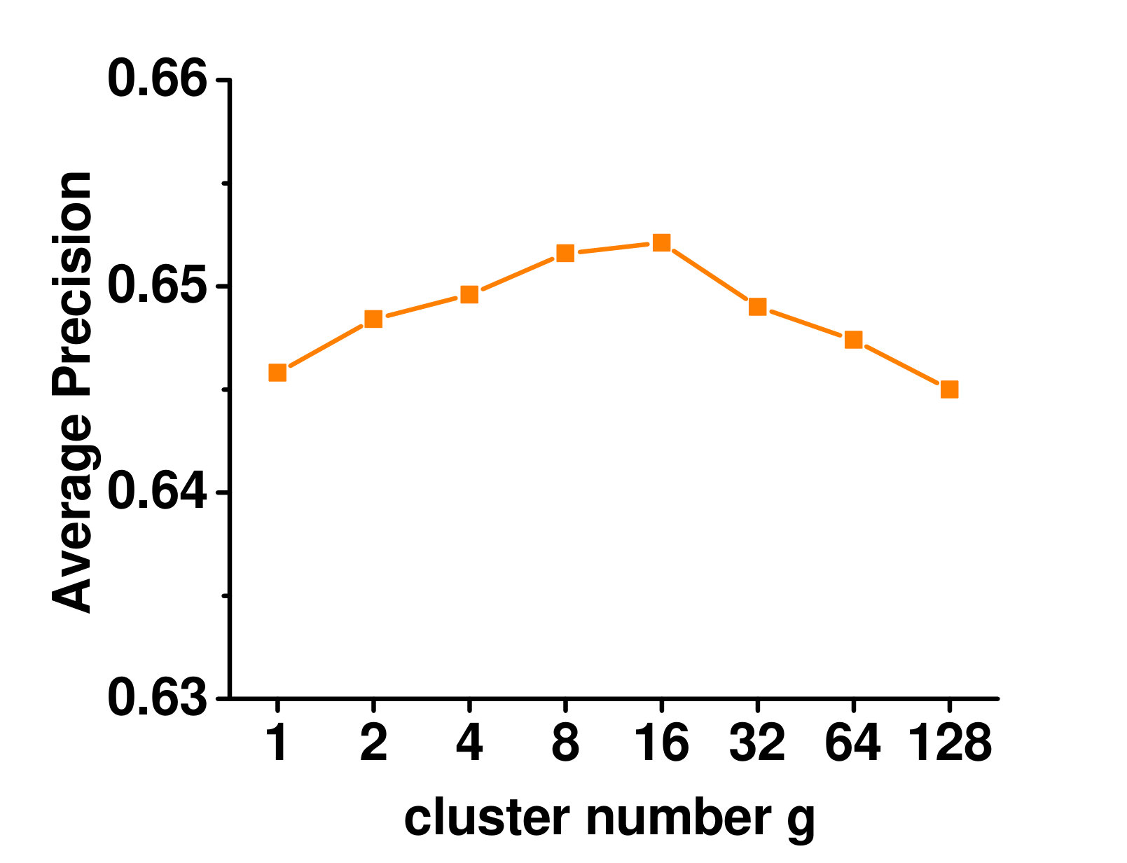 Figure 1
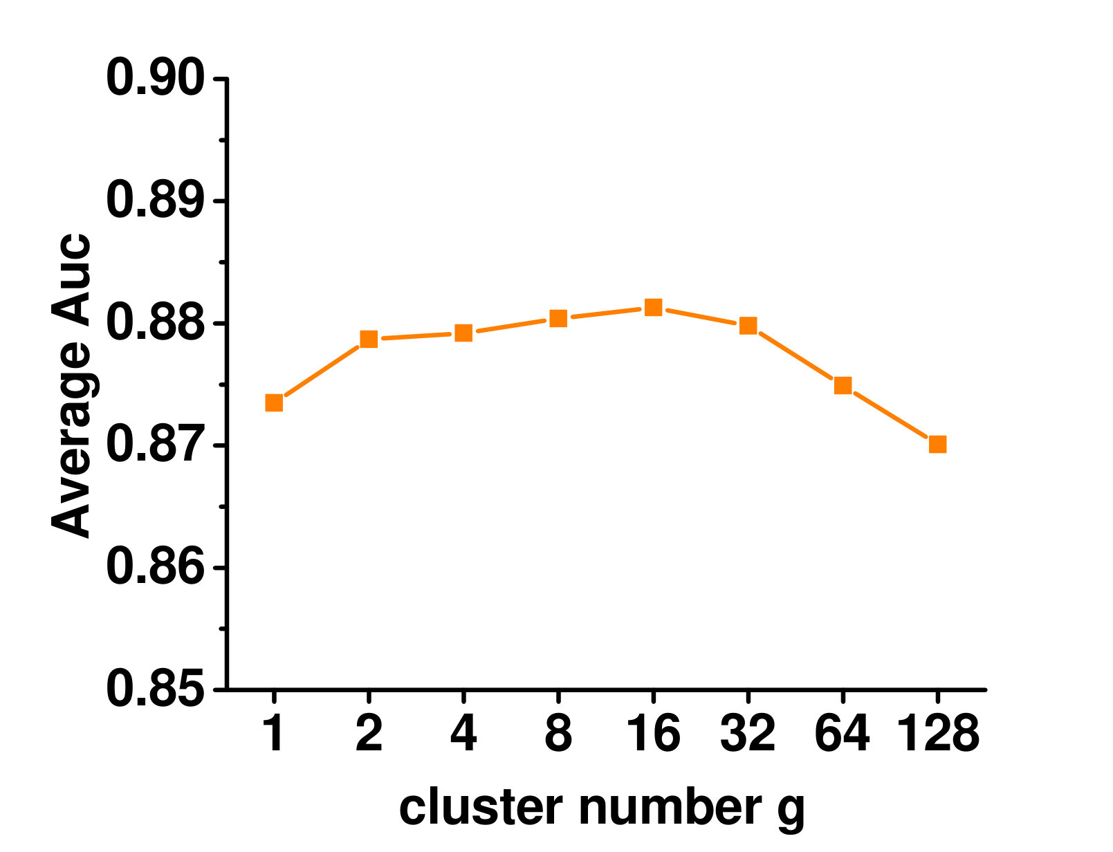 Figure 2
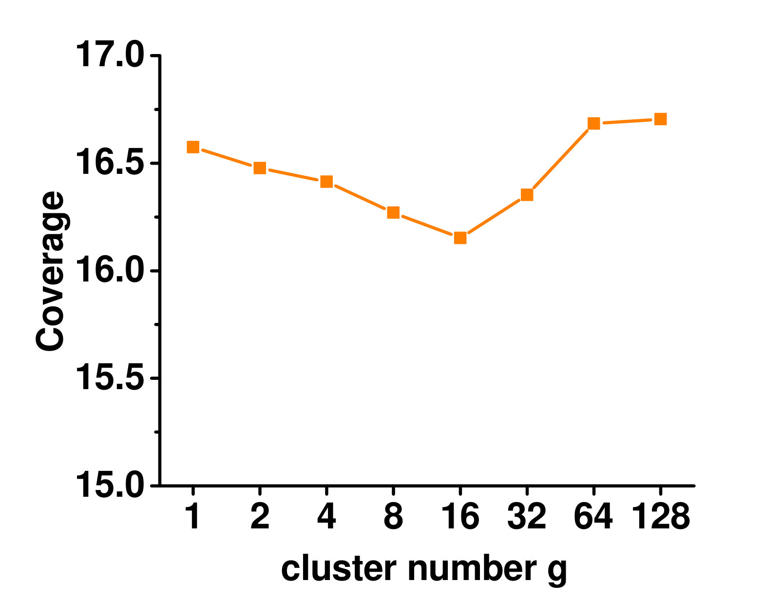 Figure 3
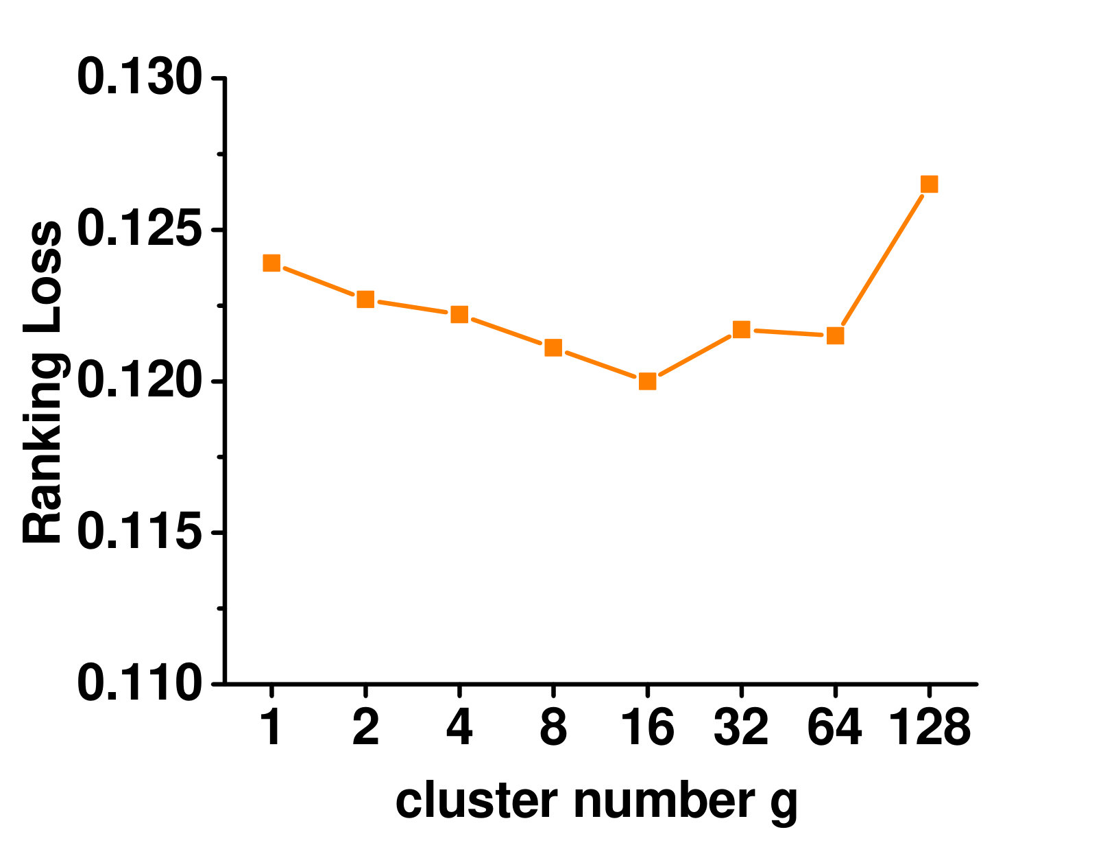 Figure 4
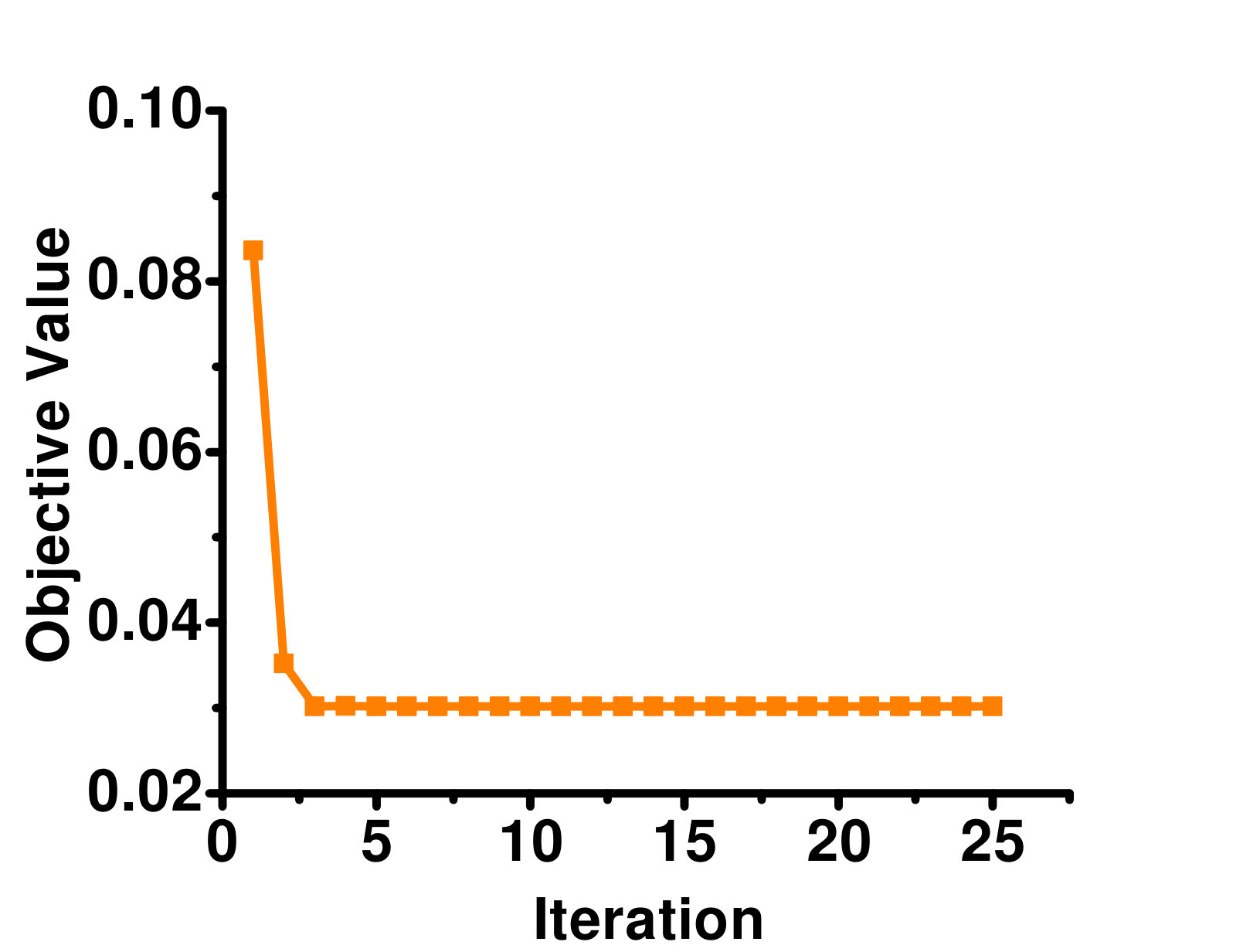 Figure 5
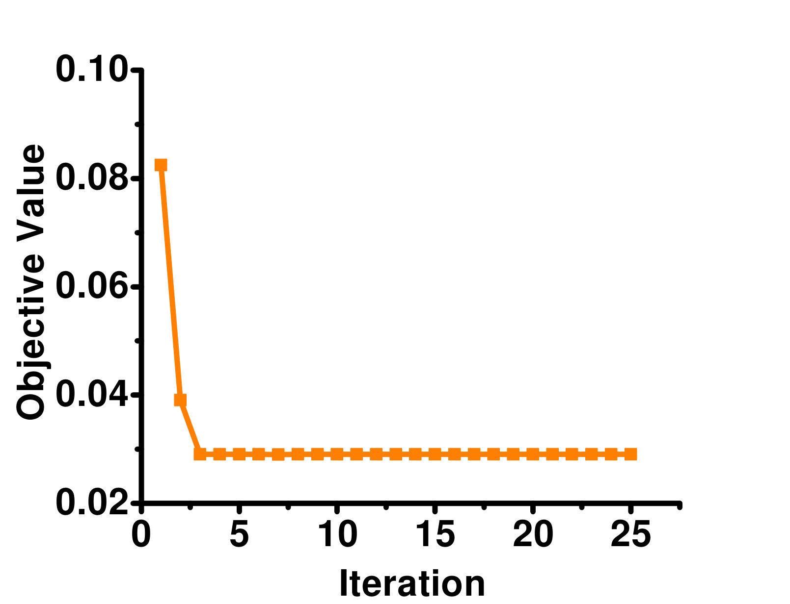 Figure 6
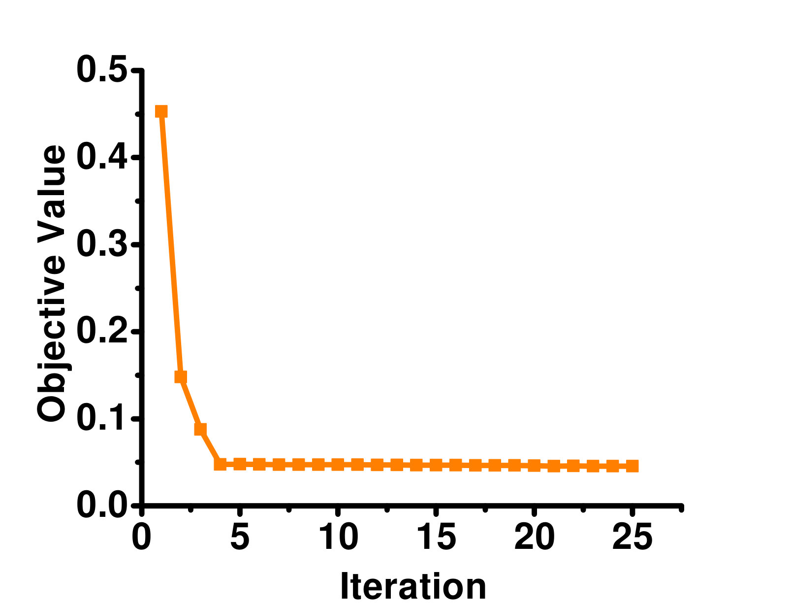 Figure 7
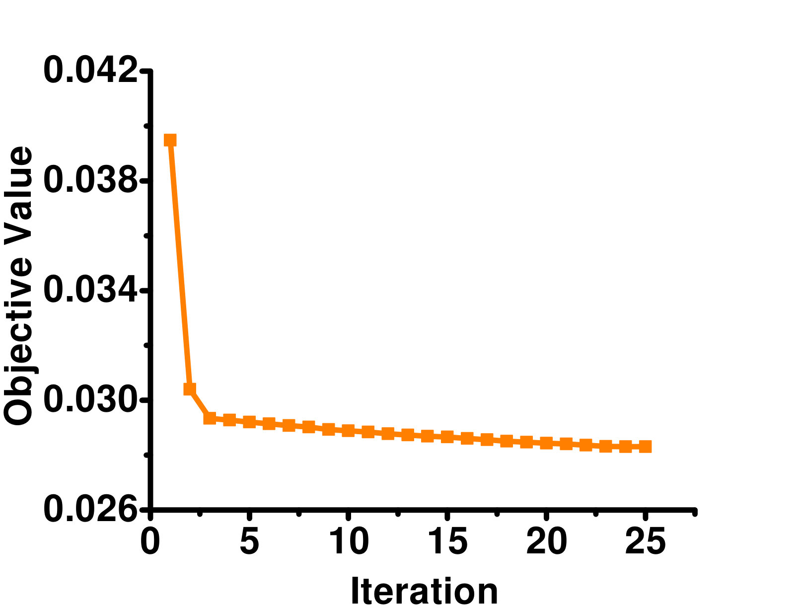 Figure 8
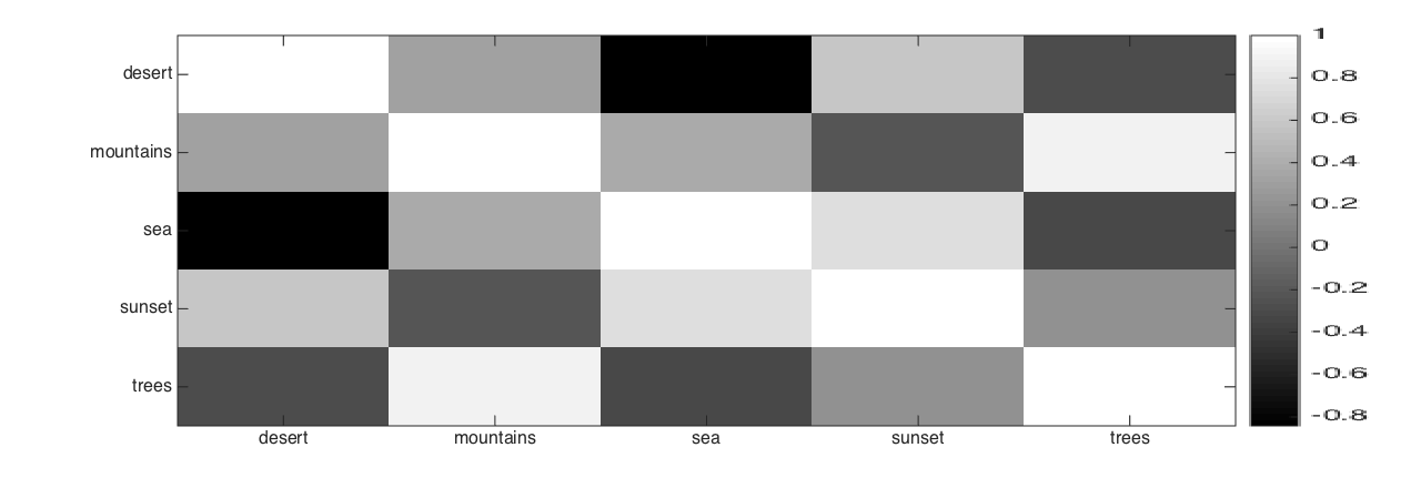 Figure 9
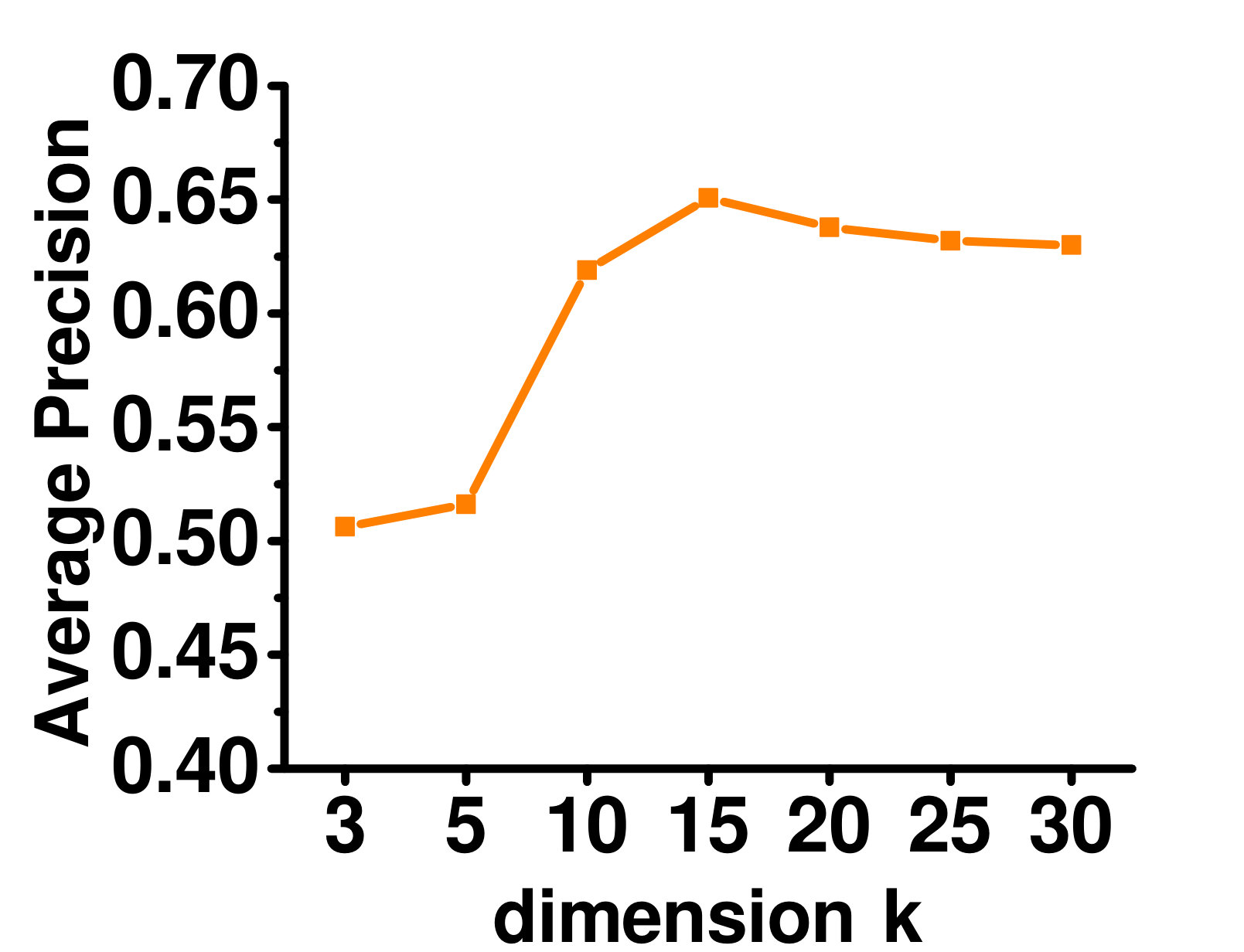 Figure 10
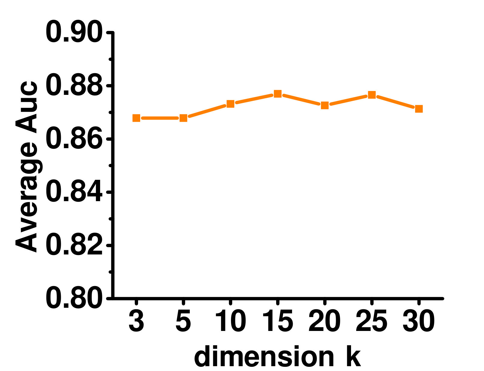 Figure 11
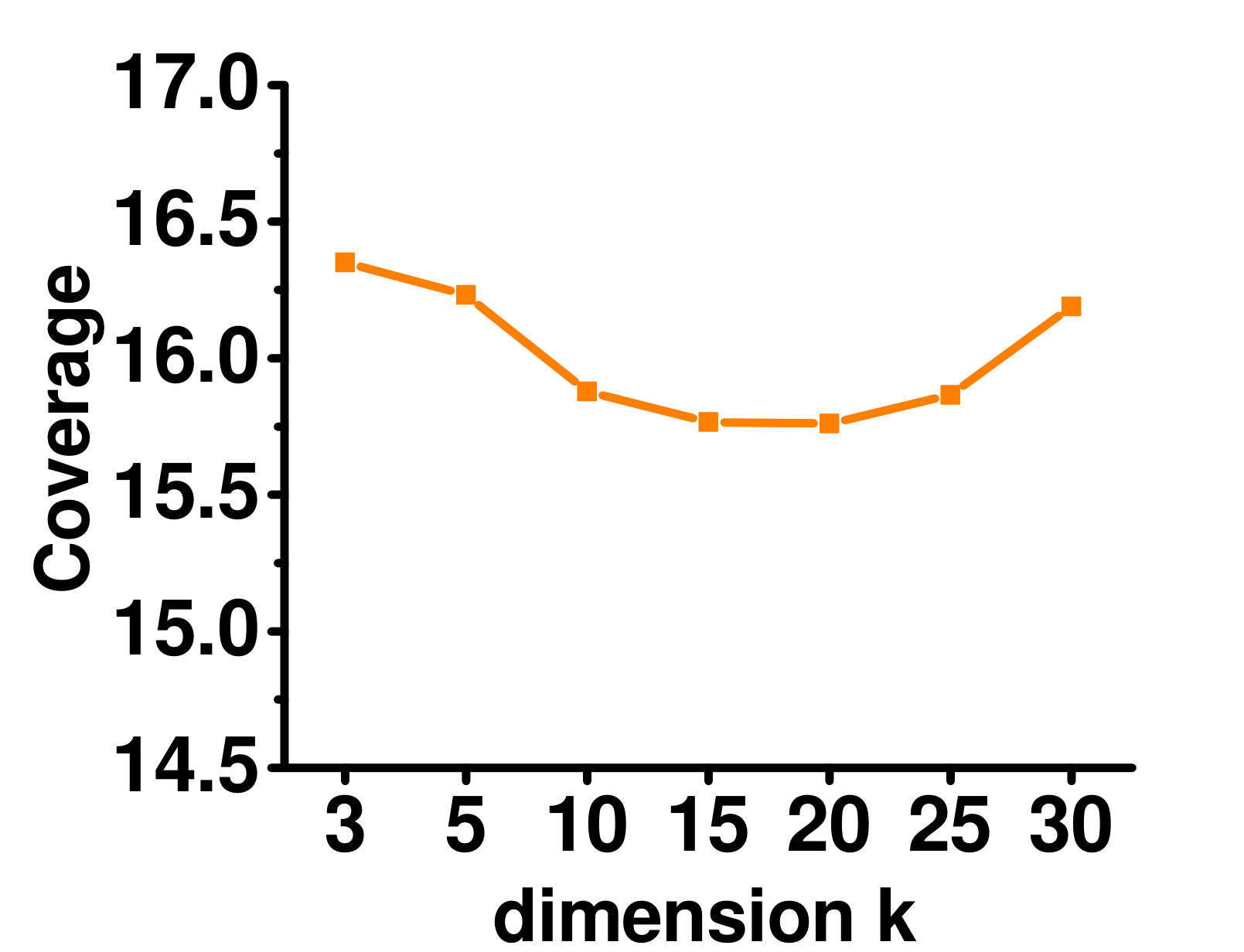 Figure 12
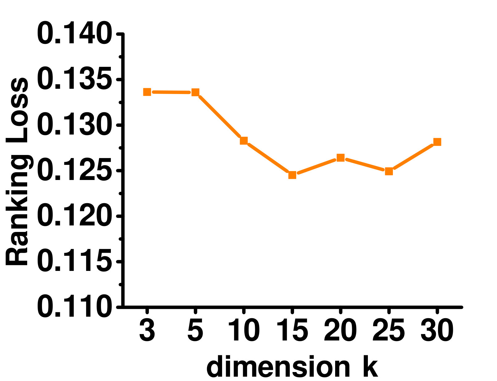 Figure 13
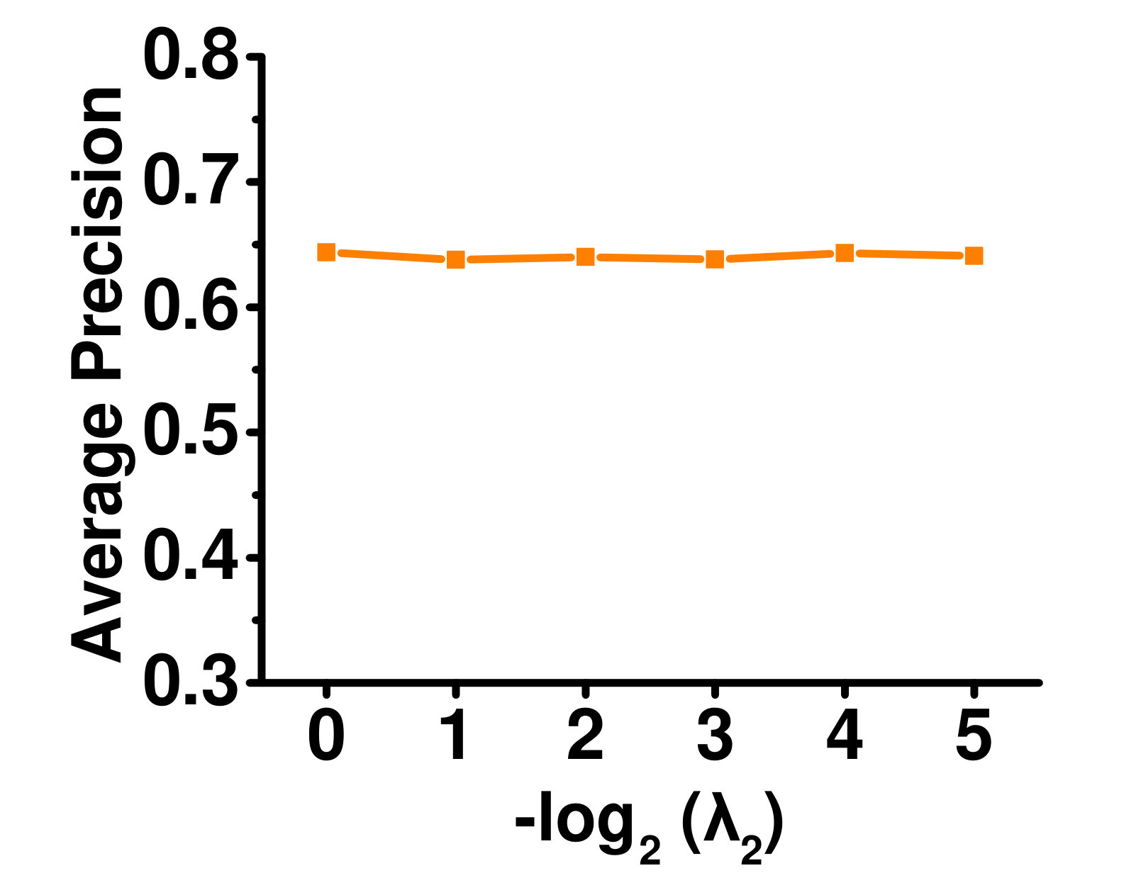 Figure 14
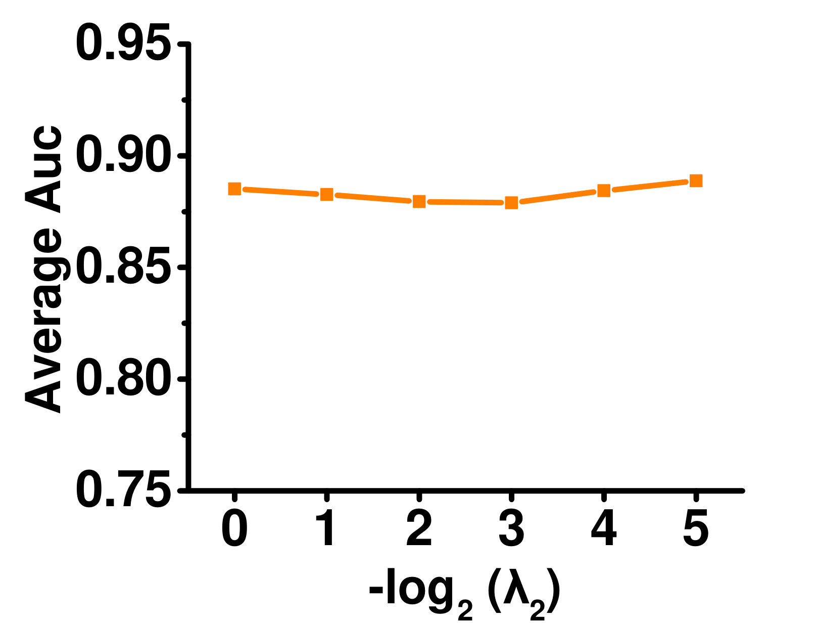 Figure 15
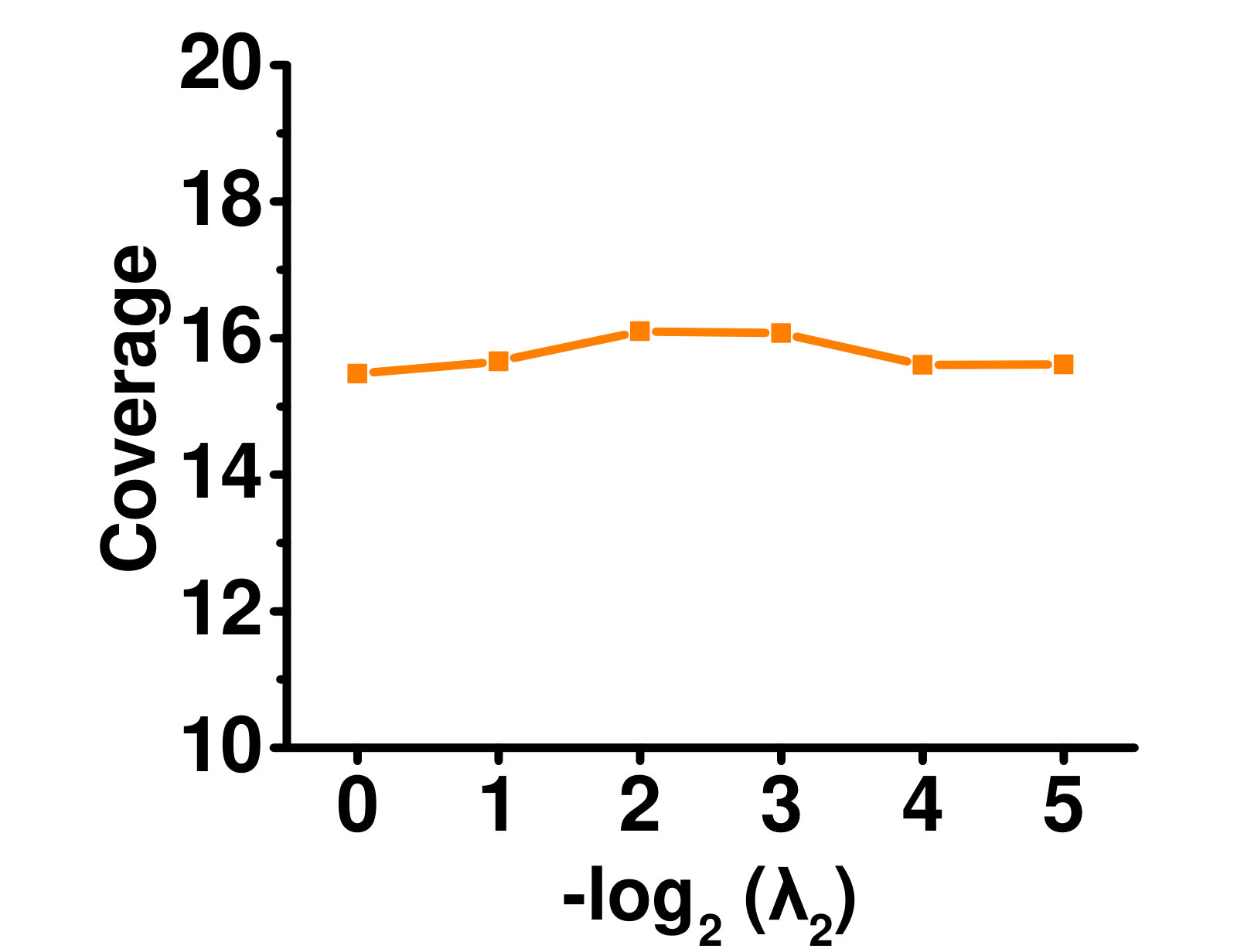 Figure 16
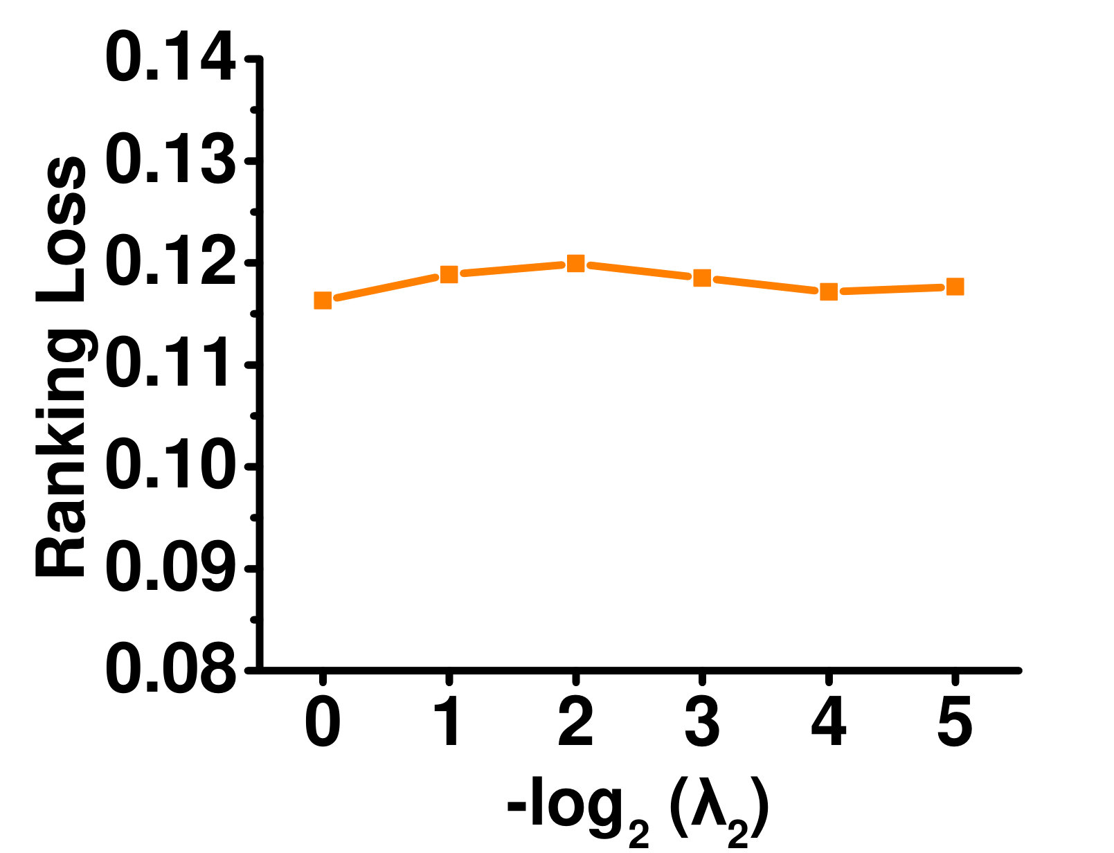 Figure 17
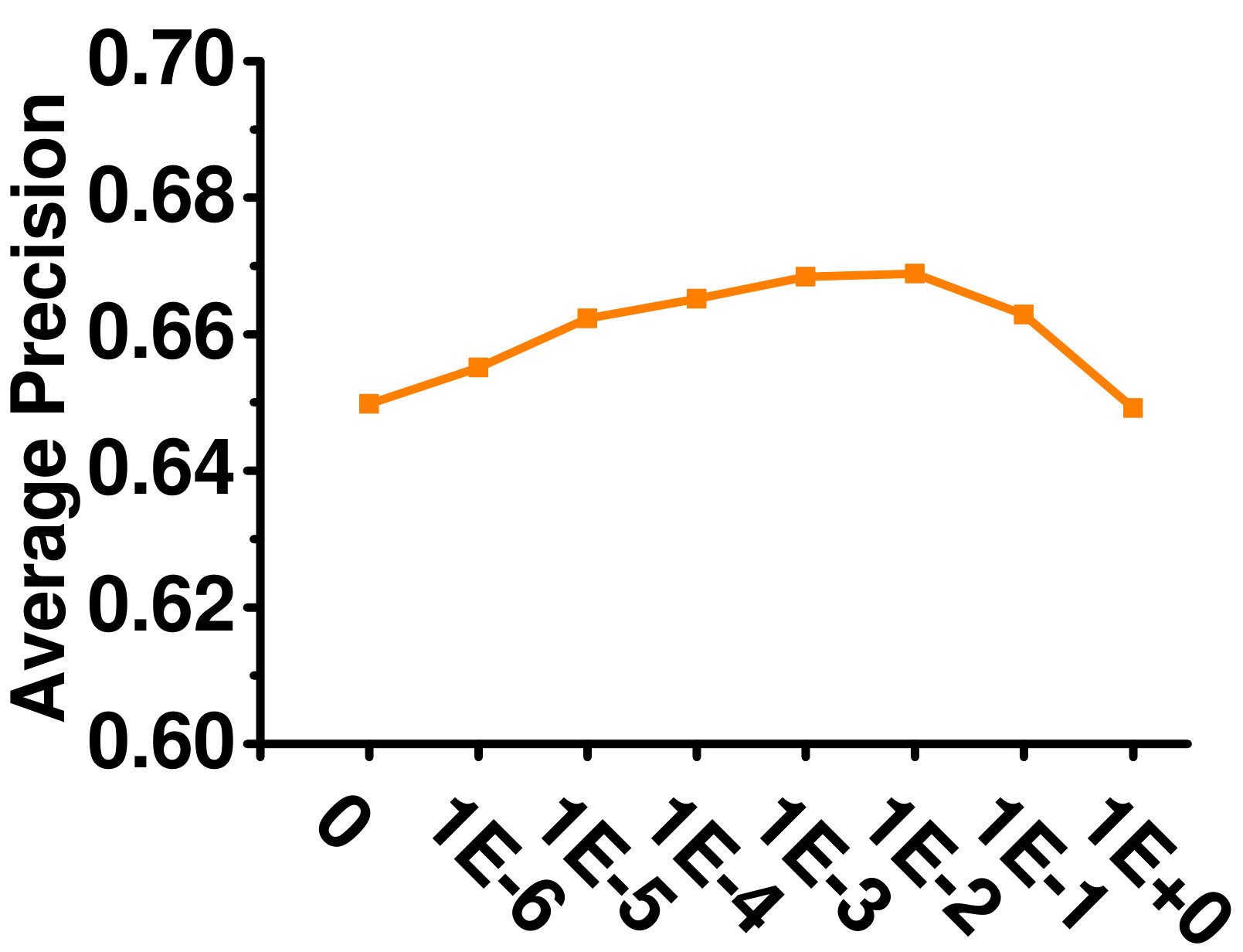 Figure 18
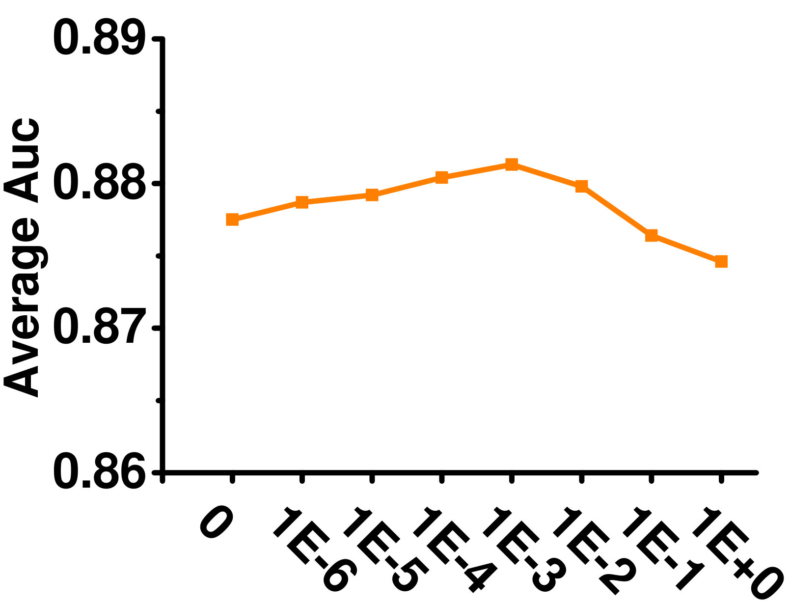 Figure 19
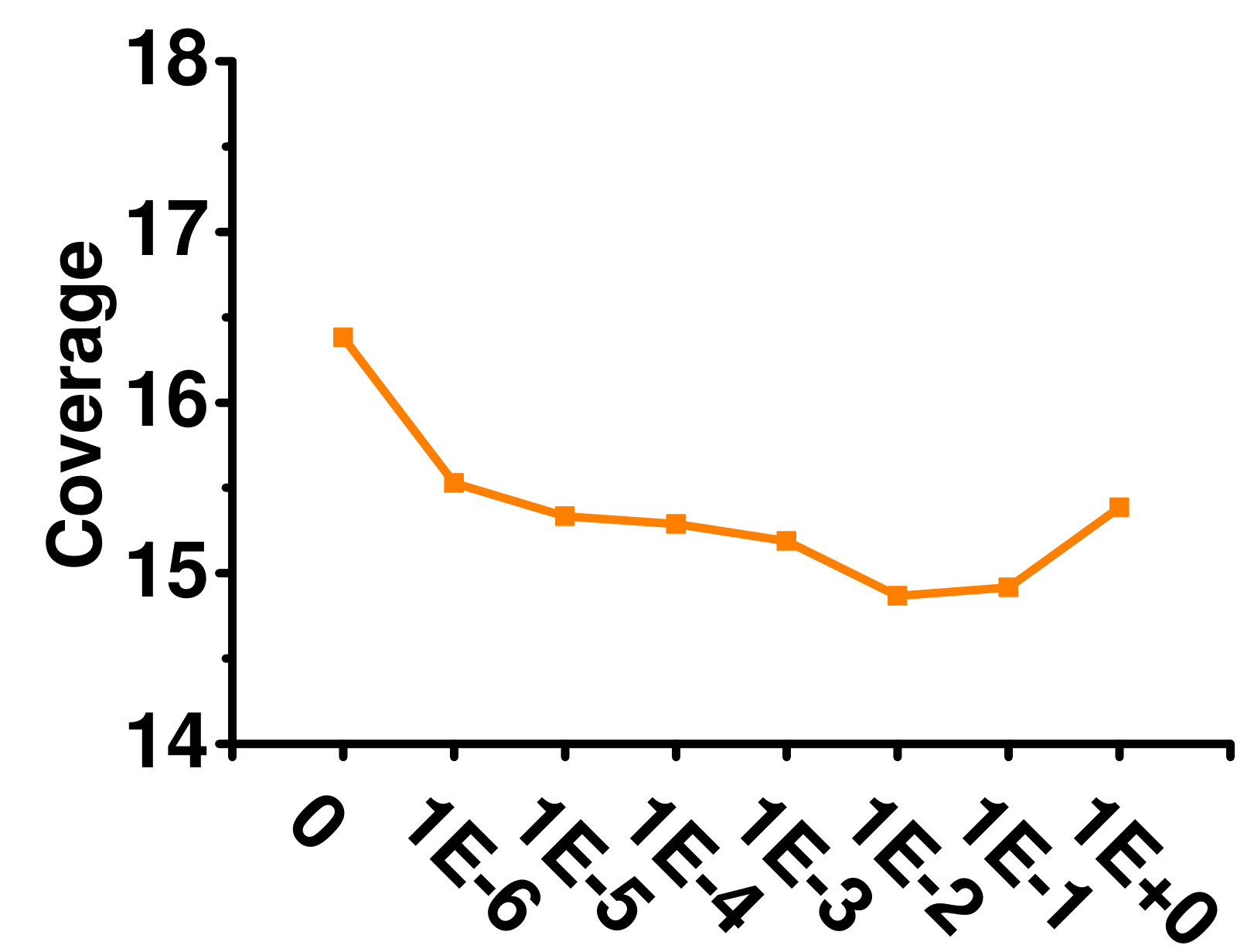 Figure 20
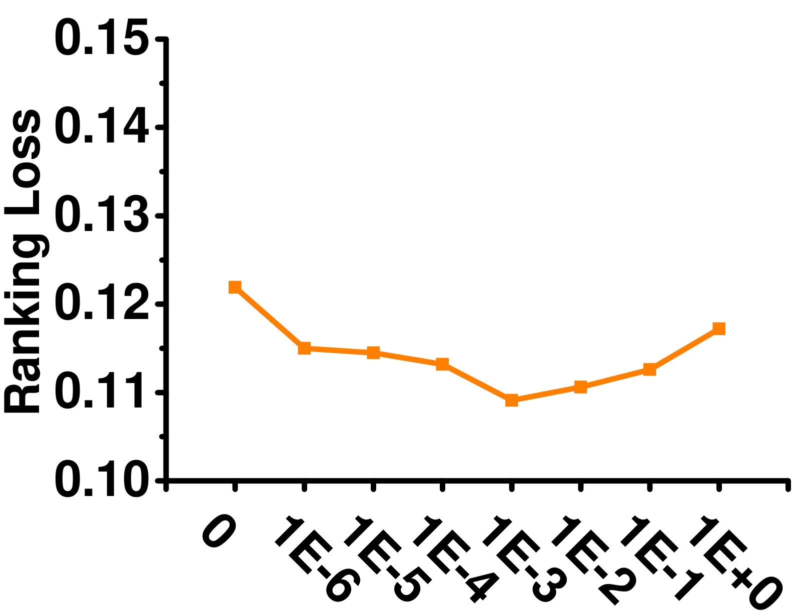 Figure 21
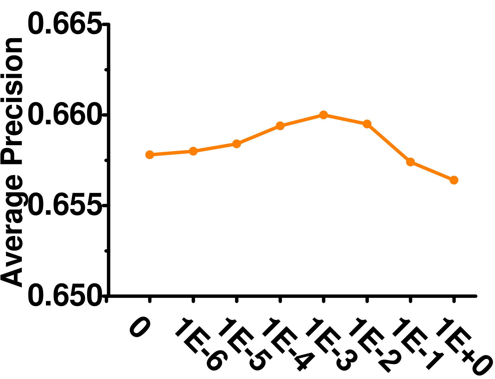 Figure 22
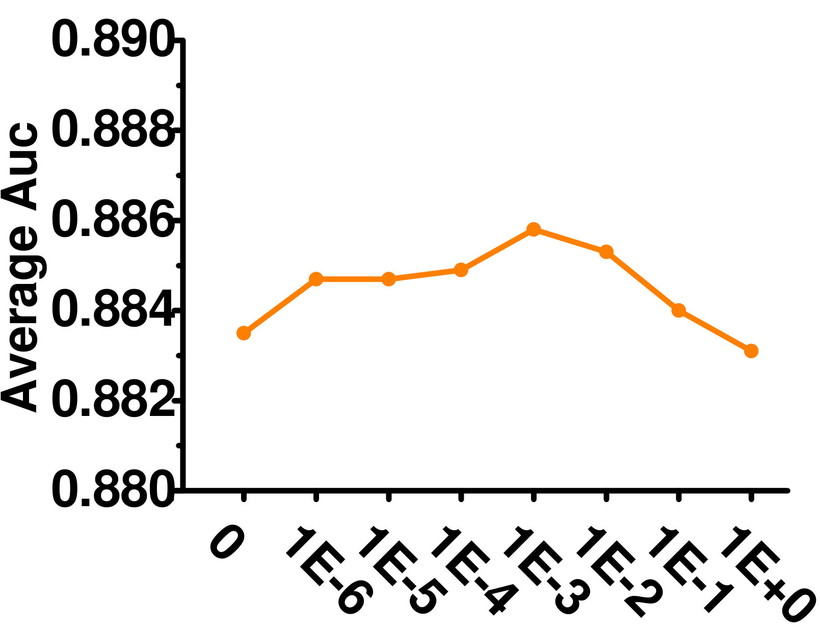 Figure 23
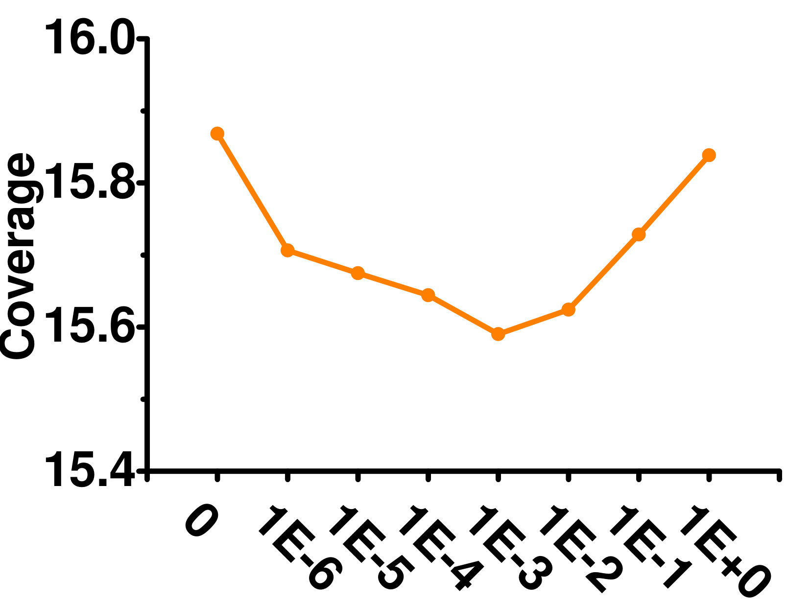 Figure 24
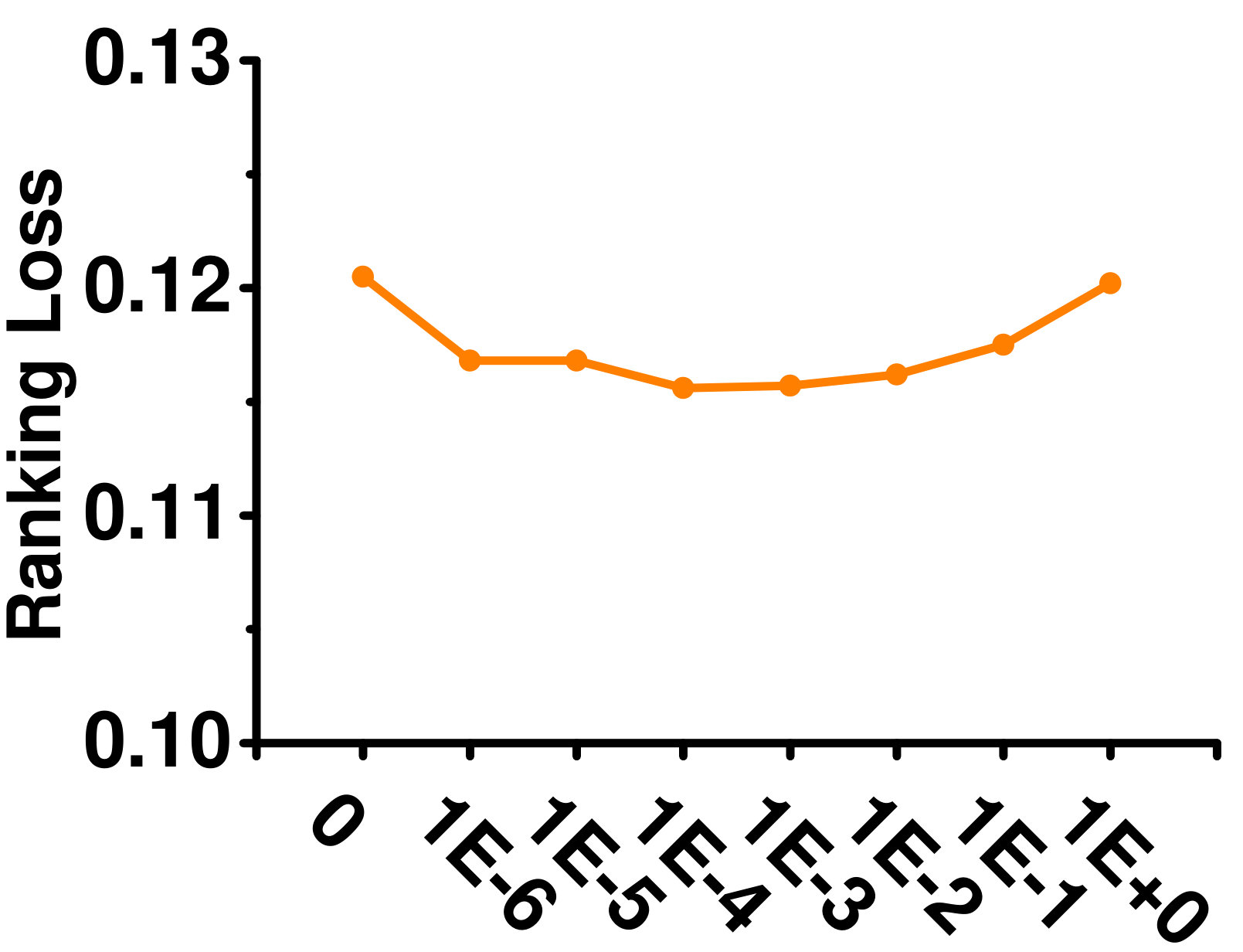 Figure 25
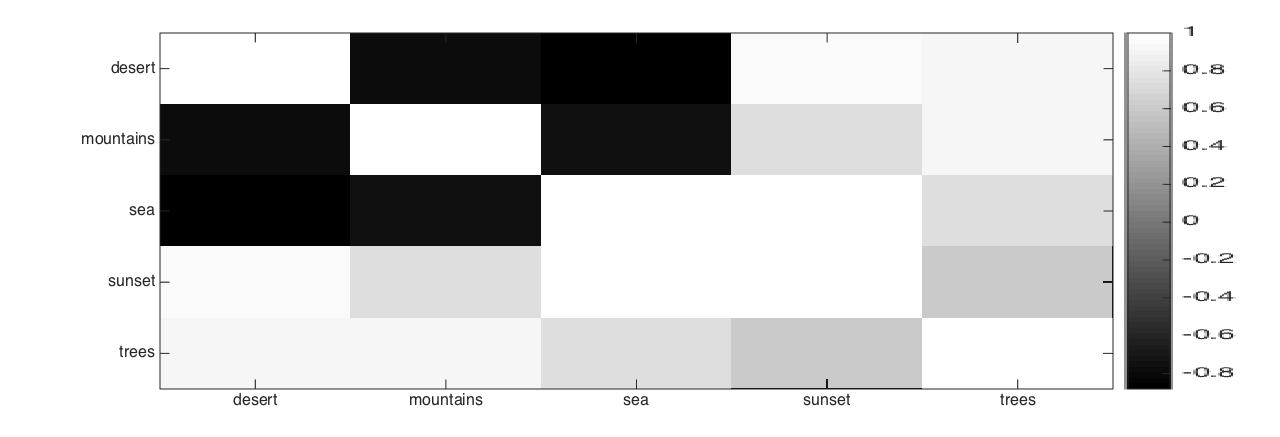 Figure 26
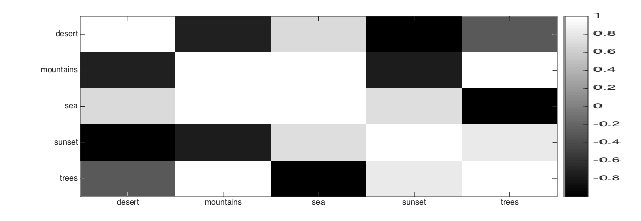 Figure 27
 Figure 28
 Figure 29
| #instance | #dim | #label | #label/instance | #instance | #dim | #label | #label/instance | ||
|---|---|---|---|---|---|---|---|---|---|
| Arts | 5,000 | 462 | 26 | 1.64 | Business | 5,000 | 438 | 30 | 1.59 |
| Computers | 5,000 | 681 | 33 | 1.51 | Education | 5,000 | 550 | 33 | 1.46 |
| Entertainment | 5,000 | 640 | 21 | 1.42 | Health | 5,000 | 612 | 32 | 1.66 |
| Recreation | 5,000 | 606 | 22 | 1.42 | Reference | 5,000 | 793 | 33 | 1.17 |
| Science | 5,000 | 743 | 40 | 1.45 | Social | 5,000 | 1,047 | 39 | 1.28 |
| Society | 5,000 | 636 | 27 | 1.69 | Enron | 1,702 | 1,001 | 53 | 3.37 |
| Corel5k | 5,000 | 499 | 374 | 3.52 | Image | 2,000 | 294 | 5 | 1.24 |
| Measure | BR | MLLOC | LEML | ML-LRC | GLOCAL | |
|---|---|---|---|---|---|---|
| Arts | Rkl () | 0.2010.005 | 0.1770.013 | 0.1700.005 | 0.1570.002 | 0.1380.002 |
| Auc () | 0.7990.006 | 0.8230.013 | 0.8330.005 | 0.8430.001 | 0.8460.005 | |
| Cvg () | 7.3470.196 | 6.7620.344 | 6.3370.243 | 5.5290.037 | 5.3470.146 | |
| Ap () | 0.5940.006 | 0.6060.006 | 0.5900.005 | 0.6000.007 | 0.6190.005 | |
| Business | Rkl () | 0.0720.005 | 0.0550.009 | 0.0560.005 | 0.0440.002 | 0.0440.002 |
| Auc () | 0.9280.005 | 0.9440.008 | 0.9450.005 | 0.9500.005 | 0.9550.003 | |
| Cvg () | 4.0870.268 | 3.2650.464 | 3.1870.270 | 2.5600.059 | 2.5590.169 | |
| Ap () | 0.8610.007 | 0.8780.011 | 0.8670.007 | 0.8700.005 | 0.8830.004 | |
| Computers | Rkl () | 0.1460.007 | 0.1340.014 | 0.1380.004 | 0.1070.002 | 0.1070.002 |
| Auc () | 0.8540.007 | 0.8660.014 | 0.8950.002 | 0.8940.002 | 0.8950.002 | |
| Cvg () | 6.6540.236 | 6.2240.480 | 6.1480.183 | 4.8930.142 | 4.8890.058 | |
| Ap () | 0.6800.007 | 0.6890.009 | 0.6690.007 | 0.6890.005 | 0.6980.004 | |
| Education | Rkl () | 0.2030.010 | 0.1580.021 | 0.1450.008 | 0.0990.002 | 0.0950.002 |
| Auc () | 0.7970.102 | 0.8420.022 | 0.8590.008 | 0.8680.006 | 0.8780.006 | |
| Cvg () | 8.9790.487 | 7.3810.765 | 6.7110.364 | 4.5310.104 | 4.5290.206 | |
| Ap () | 0.5800.010 | 0.6130.004 | 0.5960.009 | 0.6000.007 | 0.6280.009 | |
| Entertainment | Rkl () | 0.1850.006 | 0.1460.013 | 0.1540.005 | 0.1300.005 | 0.1080.004 |
| Auc () | 0.8150.006 | 0.8540.013 | 0.8520.005 | 0.8710.003 | 0.8740.005 | |
| Cvg () | 5.0060.160 | 4.2930.344 | 4.1930.139 | 3.5050.125 | 3.1140.110 | |
| Ap () | 0.6620.009 | 0.6700.005 | 0.6470.007 | 0.6610.012 | 0.6810.008 | |
| Health | Rkl () | 0.1130.001 | 0.0930.005 | 0.0910.003 | 0.0710.003 | 0.0650.002 |
| Auc () | 0.8860.003 | 0.9070.005 | 0.9130.004 | 0.9290.009 | 0.9230.007 | |
| Cvg () | 6.1930.059 | 5.4030.157 | 5.0630.128 | 3.7510.128 | 3.8580.131 | |
| Ap () | 0.7630.002 | 0.7770.004 | 0.7500.003 | 0.7550.006 | 0.7820.001 | |
| Recreation | Rkl () | 0.1970.003 | 0.1840.015 | 0.1850.001 | 0.1700.004 | 0.1550.002 |
| Auc () | 0.8020.003 | 0.8160.015 | 0.8220.002 | 0.8330.004 | 0.8400.000 | |
| Cvg () | 5.5060.089 | 5.2680.333 | 5.1100.040 | 4.5150.045 | 4.4310.048 | |
| Ap () | 0.6090.005 | 0.6200.004 | 0.5950.004 | 0.6040.003 | 0.6250.004 | |
| Reference | Rkl () | 0.1550.005 | 0.1380.008 | 0.1370.004 | 0.0920.003 | 0.0860.003 |
| Auc () | 0.8450.005 | 0.8620.008 | 0.8720.004 | 0.9000.006 | 0.8940.004 | |
| Cvg () | 6.1710.219 | 5.5140.309 | 5.2770.171 | 3.4380.133 | 3.3870.118 | |
| Ap () | 0.6850.005 | 0.6880.003 | 0.6670.003 | 0.6670.007 | 0.6880.007 | |
| Science | Rkl () | 0.1970.009 | 0.1660.017 | 0.1700.005 | 0.1310.002 | 0.1180.003 |
| Auc () | 0.8020.010 | 0.8340.018 | 0.8340.005 | 0.8600.003 | 0.8530.010 | |
| Cvg () | 10.1890.435 | 8.8670.751 | 8.8850.197 | 6.7040.122 | 6.4340.137 | |
| Ap () | 0.5680.012 | 0.5810.009 | 0.5510.008 | 0.5610.009 | 0.5800.009 | |
| Social | Rkl () | 0.1120.001 | 0.0940.013 | 0.1060.006 | 0.0750.005 | 0.0750.005 |
| Auc () | 0.8880.002 | 0.9060.013 | 0.8940.006 | 0.9170.005 | 0.9150.005 | |
| Cvg () | 6.0360.125 | 5.1470.401 | 5.5210.301 | 4.6510.102 | 4.5370.258 | |
| Ap () | 0.7240.005 | 0.7640.008 | 0.7310.005 | 0.7190.003 | 0.7580.008 | |
| Society | Rkl () | 0.2040.004 | 0.1820.006 | 0.1820.007 | 0.1420.002 | 0.1360.005 |
| Auc () | 0.7960.005 | 0.8180.006 | 0.8220.008 | 0.8400.006 | 0.8440.006 | |
| Cvg () | 8.0480.108 | 7.3920.216 | 7.4380.162 | 5.9730.108 | 5.8520.194 | |
| Ap () | 0.6100.007 | 0.6230.004 | 0.5990.006 | 0.6050.006 | 0.6330.009 | |
| Enron | Rkl () | 0.1940.006 | 0.1690.012 | 0.1590.005 | 0.1330.004 | 0.1250.004 |
| Auc () | 0.8060.006 | 0.8310.009 | 0.8510.006 | 0.8690.004 | 0.8770.005 | |
| Cvg () | 23.6180.450 | 21.7240.950 | 18.5310.707 | 16.6540.198 | 16.7370.622 | |
| Ap () | 0.5750.006 | 0.5860.009 | 0.6000.004 | 0.5910.004 | 0.6470.006 | |
| Corel5k | Rkl () | 0.2710.006 | 0.2300.012 | 0.2460.004 | 0.1700.002 | 0.1730.005 |
| Auc () | 0.6990.006 | 0.7570.012 | 0.7540.005 | 0.8250.005 | 0.8270.005 | |
| Cvg () | 261.993.15 | 201.806.71 | 184.581.72 | 137.312.49 | 136.913.21 | |
| Ap () | 0.1530.001 | 0.1820.005 | 0.1880.004 | 0.1980.003 | 0.2000.004 | |
| Image | Rkl () | 0.1810.011 | 0.1800.008 | 0.1810.012 | 0.1800.009 | 0.1790.004 |
| Auc () | 0.8120.011 | 0.8100.012 | 0.7860.005 | 0.7480.010 | 0.8190.009 | |
| Cvg () | 1.0040.050 | 0.9750.060 | 1.0000.027 | 1.0000.019 | 0.9750.054 | |
| Ap () | 0.7880.008 | 0.7940.010 | 0.7900.008 | 0.7900.010 | 0.7950.007 |
| GLObal | loCAL | GLOCAL | GLObal | loCAL | GLOCAL | ||||
|---|---|---|---|---|---|---|---|---|---|
| Art | Rkl () | 0.1370.003 | 0.1370.002 | 0.1300.005 | Bus | Rkl () | 0.0400.002 | 0.0400.002 | 0.0400.003 |
| Auc () | 0.8630.003 | 0.8630.002 | 0.8700.005 | Auc () | 0.9580.003 | 0.9580.003 | 0.9580.003 | ||
| Cvg () | 5.2860.046 | 5.2860.046 | 5.1970.065 | Cvg () | 2.5290.035 | 2.5280.040 | 2.5280.040 | ||
| Ap () | 0.6020.013 | 0.6020.010 | 0.6310.011 | Ap () | 0.8820.002 | 0.8820.002 | 0.8860.003 | ||
| Com | Rkl () | 0.0950.002 | 0.0950.002 | 0.0920.002 | Edu | Rkl () | 0.1010.002 | 0.1010.002 | 0.0970.002 |
| Auc () | 0.9050.002 | 0.9050.002 | 0.9080.001 | Auc () | 0.8990.002 | 0.8990.002 | 0.9030.002 | ||
| Cvg () | 4.4820.032 | 4.4860.040 | 4.3640.055 | Cvg () | 4.8030.033 | 4.8050.036 | 4.6720.051 | ||
| Ap () | 0.6770.003 | 0.6760.003 | 0.6780.005 | Ap () | 0.6050.003 | 0.6050.003 | 0.6240.005 | ||
| Ent | Rkl () | 0.0910.002 | 0.0910.002 | 0.0860.003 | Hea | Rkl () | 0.0540.002 | 0.0540.003 | 0.0530.004 |
| Auc () | 0.9090.002 | 0.9090.002 | 0.9140.002 | Auc () | 0.9450.003 | 0.9460.003 | 0.9470.003 | ||
| Cvg () | 2.8170.027 | 2.7970.035 | 2.7090.059 | Cvg () | 3.5080.036 | 3.5060.049 | 3.5040.041 | ||
| Ap () | 0.7480.003 | 0.7490.004 | 0.7590.006 | Ap () | 0.8100.004 | 0.8100.004 | 0.8120.006 | ||
| Rec | Rkl () | 0.1240.002 | 0.1240.002 | 0.1180.002 | Ref | Rkl () | 0.0600.002 | 0.0610.003 | 0.0540.004 |
| Auc () | 0.8710.003 | 0.8700.003 | 0.8720.004 | Auc () | 0.9400.003 | 0.9390.004 | 0.9460.004 | ||
| Cvg () | 3.7040.033 | 3.7000.037 | 3.7000.042 | Cvg () | 2.5520.043 | 2.5590.057 | 2.3250.060 | ||
| Ap () | 0.6700.004 | 0.6700.004 | 0.6720.005 | Ap () | 0.7390.004 | 0.7390.004 | 0.7830.005 | ||
| Sci | Rkl () | 0.1070.004 | 0.1080.004 | 0.1070.004 | Soc | Rkl () | 0.0630.002 | 0.0630.002 | 0.0600.002 |
| Auc () | 0.8930.004 | 0.8920.004 | 0.8930.005 | Auc () | 0.9300.002 | 0.9300.002 | 0.9340.002 | ||
| Cvg () | 5.9370.041 | 5.9410.049 | 5.8450.054 | Cvg () | 3.5580.033 | 3.5590.038 | 3.5520.049 | ||
| Ap () | 0.6080.003 | 0.6080.003 | 0.6100.003 | Ap () | 0.7970.002 | 0.7970.003 | 0.7980.003 | ||
| Soci | Rkl () | 0.1260.003 | 0.1260.005 | 0.1130.005 | Enr | Rkl () | 0.1170.002 | 0.1190.003 | 0.1050.005 |
| Auc () | 0.8740.003 | 0.8740.004 | 0.8870.005 | Auc () | 0.8830.004 | 0.8810.004 | 0.8950.004 | ||
| Cvg () | 5.5540.047 | 5.5530.053 | 5.2080.059 | Cvg () | 19.4400.833 | 19.3720.915 | 17.5111.231 | ||
| Ap () | 0.6700.004 | 0.6700.005 | 0.7110.005 | Ap () | 0.6850.005 | 0.6730.005 | 0.7060.007 | ||
| Cor | Rkl () | 0.1630.002 | 0.1630.002 | 0.1600.002 | Ima | Rkl () | 0.1970.003 | 0.1990.004 | 0.1900.004 |
| Auc () | 0.8370.002 | 0.8370.002 | 0.8400.002 | Auc () | 0.8030.003 | 0.8010.003 | 0.8100.003 | ||
| Cvg () | 130.841.01 | 131.131.21 | 128.401.30 | Cvg () | 1.0640.015 | 1.0660.021 | 1.0270.027 | ||
| Ap () | 0.2120.003 | 0.2120.003 | 0.2140.005 | Ap () | 0.7640.003 | 0.7630.004 | 0.7710.005 |
| Measure | MAXIDE | LEML | ML-LRC | GLOCAL | Measure | MAXIDE | LEML | ML-LRC | GLOCAL | ||||
|---|---|---|---|---|---|---|---|---|---|---|---|---|---|
| Art | Rkl () | 30 | 0.131 | 0.133 | 0.137 | 0.103 | Bus | Rkl () | 30 | 0.044 | 0.046 | 0.046 | 0.029 |
| 70 | 0.083 | 0.090 | 0.083 | 0.074 | 70 | 0.026 | 0.027 | 0.024 | 0.021 | ||||
| Auc () | 30 | 0.871 | 0.848 | 0.879 | 0.897 | Auc () | 30 | 0.956 | 0.954 | 0.954 | 0.971 | ||
| 70 | 0.918 | 0.912 | 0.910 | 0.928 | 70 | 0.974 | 0.973 | 0.974 | 0.979 | ||||
| Cvg () | 30 | 5.195 | 5.231 | 5.161 | 4.189 | Cvg () | 30 | 2.550 | 2.622 | 2.622 | 1.830 | ||
| 70 | 3.616 | 3.733 | 3.778 | 3.234 | 70 | 1.742 | 1.783 | 1.746 | 1.477 | ||||
| Ap () | 30 | 0.645 | 0.634 | 0.640 | 0.652 | Ap () | 30 | 0.876 | 0.878 | 0.876 | 0.893 | ||
| 70 | 0.720 | 0.720 | 0.709 | 0.720 | 70 | 0.905 | 0.901 | 0.903 | 0.908 | ||||
| Com | Rkl () | 30 | 0.101 | 0.098 | 0.097 | 0.073 | Edu | Rkl () | 30 | 0.097 | 0.093 | 0.089 | 0.069 |
| 70 | 0.059 | 0.063 | 0.061 | 0.052 | 70 | 0.061 | 0.061 | 0.061 | 0.058 | ||||
| Auc () | 30 | 0.905 | 0.908 | 0.909 | 0.933 | Auc () | 30 | 0.902 | 0.907 | 0.911 | 0.932 | ||
| 70 | 0.947 | 0.943 | 0.945 | 0.955 | 70 | 0.938 | 0.938 | 0.940 | 0.942 | ||||
| Cvg () | 30 | 4.627 | 4.586 | 4.565 | 3.511 | Cvg () | 30 | 4.672 | 4.372 | 3.914 | 3.171 | ||
| 70 | 2.912 | 3.100 | 3.095 | 2.586 | 70 | 3.113 | 3.106 | 3.000 | 2.815 | ||||
| Ap () | 30 | 0.709 | 0.700 | 0.705 | 0.726 | Ap () | 30 | 0.653 | 0.648 | 0.653 | 0.655 | ||
| 70 | 0.787 | 0.787 | 0.787 | 0.787 | 70 | 0.711 | 0.702 | 0.710 | 0.711 | ||||
| Ent | Rkl () | 30 | 0.104 | 0.103 | 0.106 | 0.085 | Hea | Rkl () | 30 | 0.060 | 0.057 | 0.054 | 0.041 |
| 70 | 0.063 | 0.063 | 0.063 | 0.062 | 70 | 0.037 | 0.036 | 0.032 | 0.030 | ||||
| Auc () | 30 | 0.898 | 0.899 | 0.899 | 0.916 | Auc () | 30 | 0.941 | 0.943 | 0.947 | 0.960 | ||
| 70 | 0.940 | 0.938 | 0.940 | 0.940 | 70 | 0.964 | 0.964 | 0.968 | 0.971 | ||||
| Cvg () | 30 | 3.058 | 2.994 | 3.022 | 2.512 | Cvg () | 30 | 3.577 | 3.462 | 3.465 | 2.567 | ||
| 70 | 1.987 | 2.051 | 2.080 | 1.957 | 70 | 2.524 | 2.465 | 2.450 | 2.152 | ||||
| Ap () | 30 | 0.704 | 0.698 | 0.698 | 0.704 | Ap () | 30 | 0.796 | 0.794 | 0.798 | 0.801 | ||
| 70 | 0.763 | 0.765 | 0.765 | 0.768 | 70 | 0.848 | 0.842 | 0.848 | 0.848 | ||||
| Rec | Rkl () | 30 | 0.130 | 0.133 | 0.135 | 0.110 | Ref | Rkl () | 30 | 0.083 | 0.083 | 0.083 | 0.063 |
| 70 | 0.078 | 0.080 | 0.080 | 0.068 | 70 | 0.048 | 0.049 | 0.049 | 0.048 | ||||
| Auc () | 30 | 0.873 | 0.870 | 0.869 | 0.895 | Auc () | 30 | 0.919 | 0.919 | 0.918 | 0.939 | ||
| 70 | 0.925 | 0.923 | 0.920 | 0.934 | 70 | 0.955 | 0.953 | 0.953 | 0.955 | ||||
| Cvg () | 30 | 3.899 | 3.919 | 4.048 | 3.291 | Cvg () | 30 | 3.436 | 3.392 | 3.372 | 2.520 | ||
| 70 | 2.560 | 2.607 | 2.620 | 2.262 | 70 | 2.039 | 2.103 | 2.195 | 1.972 | ||||
| Ap () | 30 | 0.680 | 0.663 | 0.660 | 0.681 | Ap () | 30 | 0.681 | 0.664 | 0.674 | 0.679 | ||
| 70 | 0.767 | 0.763 | 0.760 | 0.770 | 70 | 0.745 | 0.746 | 0.746 | 0.746 | ||||
| Sci | Rkl () | 30 | 0.110 | 0.111 | 0.110 | 0.086 | Soc | Rkl () | 30 | 0.069 | 0.069 | 0.063 | 0.042 |
| 70 | 0.063 | 0.071 | 0.070 | 0.063 | 70 | 0.041 | 0.040 | 0.040 | 0.026 | ||||
| Auc () | 30 | 0.889 | 0.889 | 0.889 | 0.913 | Auc () | 30 | 0.930 | 0.930 | 0.936 | 0.957 | ||
| 70 | 0.935 | 0.928 | 0.923 | 0.935 | 70 | 0.964 | 0.959 | 0.966 | 0.973 | ||||
| Cvg () | 30 | 6.193 | 6.141 | 6.271 | 4.845 | Cvg () | 30 | 3.865 | 3.920 | 3.304 | 2.443 | ||
| 70 | 3.771 | 3.914 | 3.878 | 3.751 | 70 | 2.103 | 2.386 | 2.373 | 1.663 | ||||
| Ap () | 30 | 0.615 | 0.613 | 0.614 | 0.615 | Ap () | 30 | 0.780 | 0.780 | 0.784 | 0.802 | ||
| 70 | 0.689 | 0.647 | 0.650 | 0.691 | 70 | 0.854 | 0.865 | 0.865 | 0.865 | ||||
| Soci | Rkl () | 30 | 0.129 | 0.128 | 0.123 | 0.102 | Enr | Rkl () | 30 | 0.091 | 0.115 | 0.085 | 0.075 |
| 70 | 0.074 | 0.081 | 0.073 | 0.073 | 70 | 0.042 | 0.060 | 0.040 | 0.040 | ||||
| Auc () | 30 | 0.871 | 0.872 | 0.877 | 0.898 | Auc () | 30 | 0.910 | 0.887 | 0.918 | 0.926 | ||
| 70 | 0.926 | 0.919 | 0.928 | 0.929 | 70 | 0.960 | 0.942 | 0.962 | 0.962 | ||||
| Cvg () | 30 | 5.557 | 5.459 | 5.167 | 4.496 | Cvg () | 30 | 14.24 | 16.65 | 13.45 | 12.05 | ||
| 70 | 3.641 | 3.824 | 3.608 | 3.442 | 70 | 7.961 | 10.33 | 7.480 | 7.510 | ||||
| Ap () | 30 | 0.646 | 0.629 | 0.650 | 0.652 | Ap () | 30 | 0.739 | 0.711 | 0.739 | 0.739 | ||
| 70 | 0.719 | 0.717 | 0.719 | 0.719 | 70 | 0.854 | 0.842 | 0.855 | 0.855 | ||||
| Cor | Rkl () | 30 | 0.226 | 0.214 | 0.206 | 0.185 | Ima | Rkl () | 30 | 0.302 | 0.184 | 0.175 | 0.173 |
| 70 | 0.138 | 0.131 | 0.123 | 0.125 | 70 | 0.251 | 0.148 | 0.148 | 0.148 | ||||
| Auc () | 30 | 0.773 | 0.786 | 0.794 | 0.814 | Auc () | 30 | 0.820 | 0.828 | 0.826 | 0.828 | ||
| 70 | 0.874 | 0.874 | 0.874 | 0.874 | 70 | 0.834 | 0.857 | 0.855 | 0.855 | ||||
| Cvg () | 30 | 204.90 | 182.76 | 178.60 | 153.82 | Cvg () | 30 | 1.493 | 1.104 | 0.967 | 0.950 | ||
| 70 | 103.63 | 102.42 | 102.30 | 102.30 | 70 | 0.790 | 0.760 | 0.770 | 0.760 | ||||
| Ap () | 30 | 0.275 | 0.259 | 0.275 | 0.275 | Ap () | 30 | 0.739 | 0.776 | 0.775 | 0.785 | ||
| 70 | 0.279 | 0.279 | 0.279 | 0.279 | 70 | 0.768 | 0.841 | 0.834 | 0.841 |
| Measure | MMLLOC | LEML | ML-LRC | GLOCAL | Measure | MMLLOC | LEML | ML-LRC | GLOCAL | ||||
|---|---|---|---|---|---|---|---|---|---|---|---|---|---|
| Art | Rkl () | 30 | 0.225 | 0.204 | 0.184 | 0.144 | Bus | Rkl () | 30 | 0.083 | 0.063 | 0.061 | 0.054 |
| 70 | 0.193 | 0.181 | 0.159 | 0.139 | 70 | 0.064 | 0.058 | 0.046 | 0.046 | ||||
| Auc () | 30 | 0.781 | 0.801 | 0.828 | 0.831 | Auc () | 30 | 0.917 | 0.928 | 0.937 | 0.937 | ||
| 70 | 0.819 | 0.825 | 0.838 | 0.840 | 70 | 0.935 | 0.942 | 0.950 | 0.952 | ||||
| Cvg () | 30 | 9.033 | 7.369 | 6.281 | 5.867 | Cvg () | 30 | 4.643 | 3.954 | 3.279 | 2.863 | ||
| 70 | 7.262 | 6.431 | 5.432 | 5.352 | 70 | 3.670 | 3.303 | 2.580 | 2.579 | ||||
| Ap () | 30 | 0.529 | 0.503 | 0.517 | 0.572 | Ap () | 30 | 0.843 | 0.866 | 0.858 | 0.879 | ||
| 70 | 0.583 | 0.589 | 0.588 | 0.607 | 70 | 0.861 | 0.870 | 0.870 | 0.881 | ||||
| Com | Rkl () | 30 | 0.201 | 0.179 | 0.152 | 0.154 | Edu | Rkl () | 30 | 0.187 | 0.176 | 0.144 | 0.137 |
| 70 | 0.150 | 0.141 | 0.115 | 0.113 | 70 | 0.165 | 0.151 | 0.113 | 0.111 | ||||
| Auc () | 30 | 0.849 | 0.880 | 0.873 | 0.883 | Auc () | 30 | 0.815 | 0.817 | 0.845 | 0.846 | ||
| 70 | 0.868 | 0.894 | 0.895 | 0.896 | 70 | 0.844 | 0.842 | 0.860 | 0.860 | ||||
| Cvg () | 30 | 8.808 | 7.392 | 6.052 | 5.798 | Cvg () | 30 | 11.089 | 9.672 | 6.350 | 6.338 | ||
| 70 | 6.871 | 6.306 | 5.000 | 4.976 | 70 | 8.096 | 7.595 | 5.075 | 5.070 | ||||
| Ap () | 30 | 0.631 | 0.646 | 0.636 | 0.669 | Ap () | 30 | 0.538 | 0.537 | 0.543 | 0.592 | ||
| 70 | 0.674 | 0.665 | 0.667 | 0.691 | 70 | 0.586 | 0.591 | 0.600 | 0.622 | ||||
| Ent | Rkl () | 30 | 0.229 | 0.175 | 0.152 | 0.122 | Hea | Rkl () | 30 | 0.137 | 0.095 | 0.085 | 0.085 |
| 70 | 0.164 | 0.159 | 0.129 | 0.109 | 70 | 0.109 | 0.074 | 0.071 | 0.065 | ||||
| Auc () | 30 | 0.832 | 0.826 | 0.849 | 0.859 | Auc () | 30 | 0.894 | 0.896 | 0.907 | 0.906 | ||
| 70 | 0.842 | 0.850 | 0.870 | 0.871 | 70 | 0.901 | 0.920 | 0.920 | 0.920 | ||||
| Cvg () | 30 | 6.029 | 5.755 | 4.170 | 4.153 | Cvg () | 30 | 7.104 | 6.248 | 4.924 | 4.814 | ||
| 70 | 4.857 | 4.643 | 3.483 | 3.117 | 70 | 5.866 | 5.167 | 3.960 | 3.963 | ||||
| Ap () | 30 | 0.601 | 0.601 | 0.601 | 0.645 | Ap () | 30 | 0.727 | 0.715 | 0.720 | 0.752 | ||
| 70 | 0.635 | 0.645 | 0.643 | 0.670 | 70 | 0.762 | 0.770 | 0.766 | 0.775 | ||||
| Rec | Rkl () | 30 | 0.266 | 0.245 | 0.202 | 0.165 | Ref | Rkl () | 30 | 0.199 | 0.187 | 0.137 | 0.098 |
| 70 | 0.204 | 0.196 | 0.167 | 0.156 | 70 | 0.155 | 0.145 | 0.098 | 0.086 | ||||
| Auc () | 30 | 0.785 | 0.828 | 0.802 | 0.839 | Auc () | 30 | 0.851 | 0.847 | 0.868 | 0.886 | ||
| 70 | 0.800 | 0.837 | 0.836 | 0.845 | 70 | 0.861 | 0.869 | 0.895 | 0.898 | ||||
| Cvg () | 30 | 7.084 | 6.842 | 5.397 | 4.545 | Cvg () | 30 | 7.549 | 6.463 | 5.052 | 3.367 | ||
| 70 | 5.952 | 5.685 | 4.490 | 4.430 | 70 | 6.419 | 6.130 | 3.694 | 3.348 | ||||
| Ap () | 30 | 0.547 | 0.540 | 0.540 | 0.573 | Ap () | 30 | 0.631 | 0.609 | 0.611 | 0.638 | ||
| 70 | 0.597 | 0.567 | 0.600 | 0.614 | 70 | 0.675 | 0.653 | 0.653 | 0.672 | ||||
| Sci | Rkl () | 30 | 0.257 | 0.203 | 0.169 | 0.144 | Soc | Rkl () | 30 | 0.149 | 0.089 | 0.095 | 0.075 |
| 70 | 0.189 | 0.174 | 0.134 | 0.129 | 70 | 0.108 | 0.079 | 0.076 | 0.073 | ||||
| Auc () | 30 | 0.827 | 0.827 | 0.830 | 0.837 | Auc () | 30 | 0.906 | 0.906 | 0.905 | 0.913 | ||
| 70 | 0.840 | 0.849 | 0.850 | 0.850 | 70 | 0.910 | 0.900 | 0.914 | 0.914 | ||||
| Cvg () | 30 | 12.805 | 10.587 | 8.794 | 6.809 | Cvg () | 30 | 7.652 | 7.567 | 6.308 | 6.088 | ||
| 70 | 9.960 | 9.501 | 6.900 | 6.416 | 70 | 5.886 | 5.386 | 5.103 | 4.929 | ||||
| Ap () | 30 | 0.503 | 0.479 | 0.485 | 0.531 | Ap () | 30 | 0.712 | 0.682 | 0.700 | 0.738 | ||
| 70 | 0.569 | 0.551 | 0.570 | 0.574 | 70 | 0.748 | 0.719 | 0.728 | 0.761 | ||||
| Soci | Rkl () | 30 | 0.252 | 0.202 | 0.175 | 0.139 | Enr | Rkl () | 30 | 0.179 | 0.172 | 0.173 | 0.149 |
| 70 | 0.208 | 0.194 | 0.141 | 0.136 | 70 | 0.170 | 0.162 | 0.152 | 0.129 | ||||
| Auc () | 30 | 0.804 | 0.808 | 0.826 | 0.826 | Auc () | 30 | 0.820 | 0.830 | 9,843 | 0.853 | ||
| 70 | 0.816 | 0.816 | 0.840 | 0.840 | 70 | 0.829 | 0.839 | 0.849 | 0.872 | ||||
| Cvg () | 30 | 9.550 | 8.637 | 6.944 | 5.816 | Cvg () | 30 | 22.72 | 21.41 | 20.42 | 19.01 | ||
| 70 | 8.227 | 7.638 | 5.750 | 5.750 | 70 | 21.90 | 19.53 | 18.17 | 17.16 | ||||
| Ap () | 30 | 0.569 | 0.563 | 0.565 | 0.601 | Ap () | 30 | 0.580 | 0.582 | 0.580 | 0.589 | ||
| 70 | 0.606 | 0.589 | 0.590 | 0.625 | 70 | 0.585 | 0.601 | 0.607 | 0.635 | ||||
| Cor | Rkl () | 30 | 0.332 | 0.308 | 0.331 | 0.285 | Ima | Rkl () | 30 | 0.224 | 0.204 | 0.220 | 0.200 |
| 70 | 0.248 | 0.250 | 0.199 | 0.194 | 70 | 0.195 | 0.188 | 0.197 | 0.187 | ||||
| Auc () | 30 | 0.673 | 0.693 | 0.670 | 0.714 | Auc () | 30 | 0.796 | 0.795 | 0.800 | 0.801 | ||
| 70 | 0.747 | 0.749 | 0.801 | 0.805 | 70 | 0.812 | 0.811 | 0.810 | 0.813 | ||||
| Cvg () | 30 | 275.41 | 233.83 | 240.17 | 211.84 | Cvg () | 30 | 1.160 | 1.103 | 1.131 | 1.070 | ||
| 70 | 212.84 | 190.83 | 160.59 | 151.23 | 70 | 1.066 | 1.030 | 1.040 | 1.025 | ||||
| Ap () | 30 | 0.158 | 0.166 | 0.165 | 0.174 | Ap () | 30 | 0.745 | 0.752 | 0.744 | 0.760 | ||
| 70 | 0.176 | 0.185 | 0.188 | 0.192 | 70 | 0.768 | 0.772 | 0.770 | 0.777 |
| MBR | MMLLOC | LEML | ML-LRC | GLOCAL | ||||||||||||||
|---|---|---|---|---|---|---|---|---|---|---|---|---|---|---|---|---|---|---|
| A | F | R | A | F | C | I | R | A | I | R | A | I | R | A | C | I | R | |
| Arts | 109 | 8 | 101 | 107 | 8 | 1 | 0 | 98 | 34 | 0 | 34 | 87 | 0 | 87 | 47 | 1 | 20 | 26 |
| Business | 38 | 6 | 32 | 104 | 6 | 1 | 0 | 97 | 35 | 0 | 35 | 82 | 0 | 82 | 49 | 1 | 24 | 24 |
| Computers | 78 | 11 | 67 | 121 | 11 | 1 | 0 | 109 | 46 | 0 | 46 | 94 | 0 | 94 | 53 | 1 | 31 | 21 |
| Education | 60 | 8 | 52 | 115 | 8 | 1 | 0 | 106 | 45 | 0 | 45 | 64 | 0 | 64 | 45 | 1 | 29 | 15 |
| Entertainment | 66 | 6 | 60 | 91 | 6 | 1 | 0 | 84 | 42 | 0 | 42 | 73 | 0 | 73 | 53 | 2 | 22 | 29 |
| Health | 64 | 11 | 53 | 116 | 11 | 1 | 0 | 104 | 41 | 0 | 41 | 75 | 0 | 75 | 67 | 1 | 32 | 34 |
| Recreation | 63 | 4 | 59 | 97 | 5 | 1 | 0 | 91 | 46 | 0 | 46 | 55 | 0 | 55 | 51 | 2 | 22 | 27 |
| Reference | 75 | 14 | 61 | 131 | 15 | 9 | 0 | 107 | 38 | 0 | 38 | 91 | 0 | 91 | 78 | 8 | 32 | 38 |
| Science | 101 | 15 | 86 | 133 | 15 | 1 | 0 | 117 | 53 | 0 | 53 | 103 | 0 | 103 | 77 | 2 | 32 | 43 |
| Social | 163 | 36 | 127 | 149 | 33 | 8 | 0 | 108 | 37 | 0 | 37 | 147 | 0 | 147 | 90 | 7 | 35 | 48 |
| Society | 83 | 8 | 75 | 106 | 8 | 1 | 0 | 97 | 32 | 0 | 32 | 117 | 0 | 117 | 44 | 2 | 18 | 24 |
| Enron | 47 | 10 | 37 | 59 | 10 | 1 | 0 | 48 | 38 | 0 | 38 | 78 | 0 | 78 | 69 | 1 | 25 | 43 |
| Corel5k | 458 | 272 | 186 | 1529 | 268 | 1 | 0 | 1260 | 307 | 0 | 307 | 709 | 0 | 709 | 413 | 1 | 78 | 344 |
| Image | 5 | 1 | 4 | 25 | 2 | 1 | 0 | 22 | 28 | 0 | 28 | 14 | 0 | 14 | 15 | 1 | 5 | 9 |
Peer Reviews
No public reviews on file for this paper yet. If you reviewed it on a platform where reviews are public (OpenReview, ICLR, NeurIPS, ICML), you can paste yours below so the community can read it here.
Videos
No videos yet. Explain this paper in a talk, walkthrough, or lecture? Add one.
Taxonomy
TopicsText and Document Classification Technologies · Natural Language Processing Techniques · Music and Audio Processing
Multi-Label Learning with
Global and Local Label Correlation
Yue Zhu1
James T. Kwok2
Zhi-Hua Zhou1
1 National Key Laboratory for Novel Software Technology
Nanjing University, Nanjing 210093, China
Email: {zhuy, zhouzh}@lamda.nju.edu.cn
2the Department of Computer Science and Engineering
Hong Kong University of Science and Technology, Hong Kong
Email: [email protected]
Abstract
It is well-known that exploiting label correlations is important to multi-label learning. Existing approaches either assume that the label correlations are global and shared by all instances; or that the label correlations are local and shared only by a data subset. In fact, in the real-world applications, both cases may occur that some label correlations are globally applicable and some are shared only in a local group of instances. Moreover, it is also a usual case that only partial labels are observed, which makes the exploitation of the label correlations much more difficult. That is, it is hard to estimate the label correlations when many labels are absent. In this paper, we propose a new multi-label approach GLOCAL dealing with both the full-label and the missing-label cases, exploiting global and local label correlations simultaneously, through learning a latent label representation and optimizing label manifolds. The extensive experimental studies validate the effectiveness of our approach on both full-label and missing-label data.
keywords:
Global and local label correlation, label manifold, missing labels, multi-label learning.
\cortext
[cor1]Corresponding author.
1 Introduction
In real-world classification applications, an instance is often associated with more than one class labels. For example, a scene image can be annotated with several tags boutell2004learning , a document may belong to multiple topics ueda2002parametric , and a piece of music may be associated with different genres turnbull2008semantic . Thus, multi-label learning has attracted a lot of attention in recent years zhang2014review .
Current studies on multi-label learning try to incorporate label correlations of different orders zhang2014review . However, existing approaches mostly focus on global label correlations shared by all instances furnkranz2008multilabel ; ji2008extracting ; read2011classifier . For example, labels “fish” and “ocean” are highly correlated, and so are “stock” and “finance”. On the other hand, certain label correlations are only shared by a local data subset huang2012 . For example, “apple” is related to “fruit” in gourmet magazines, but is related to “digital devices” in technology magazines. Previous studies focus on exploiting either global or local label correlations. However, considering both of them is obviously more beneficial and desirable.
Another problem with label correlations is that they are usually difficult to specify manually. As label correlations may vary in different contexts and there is no unified measure for specifying appropriate correlations, they are usually estimated from the observed data. Some approaches learn the label hierarchies by hierarchical clustering Punera2005Automatically or Bayesian network structure learning zhang2010multi . However, the hierarchical structure may not exist in some applications. For example, labels such as “desert”, “mountains”, “sea”, “sunset” and “trees” do not have any natural hierarchical correlations, and label hierarchies may not be useful. Others estimate label correlations by the co-occurrence of labels in training data NIPS2011_4239 . However, it may cause overfitting. Moreover, co-occurrence is less meaningful for labels with very few positive instances.
In multi-label learning, some labels may be missing from the training set. For example, human labelers may ignore object classes they do not know or of little interest. Recently, multi-label learning with missing labels has become a hot topic. Xu et al. xu2013speedup and Yu et al. Yu2014 considered using the low-rank structure on the instance-label mapping. A more direct approach to model the label dependency approximates the label matrix as a product of two low-rank matrices goldberg2010transduction . This leads to simpler recovery of the missing labels, and produces a latent representation of the label matrix.
In the missing label cases, estimation of label correlation becomes even more difficult, as the observed label distribution is different from the true one. As a result, the aforementioned methods (based on hierarchical clustering and co-occurrence, for example) will produce biased estimates of label correlations.
In this paper, we propose a new approach called “Multi-Label Learning with GLObal and loCAL Correlation” (GLOCAL), which simultaneously recovers the missing labels, trains the linear classifiers and exploits both global and local label correlations. It learns a latent label representation. Classifier outputs are encouraged to be similar on highly positively correlated labels, and dissimilar on highly negatively correlated labels. We do not assume the presence of external knowledge sources specifying the label correlations. Instead, these correlations are learned simultaneously with the latent label representations and instance-label mapping.
The rest of the paper is organized as follows. In Section 2, related works of multi-label learning with label correlations are introduced. In Section 3, the problem formulation and the GLOCAL approach are proposed. Experimental results are presented in Section 4. Finally, Section 5 concludes the work.
Notations For a matrix , denotes its transpose, is its trace, is its Frobenius norm, and returns a vector containing the diagonal elements of . For two matrices and , denotes the Hadamard (element-wise) product. For a vector , is its -norm, and returns a diagonal matrix with on the diagonal.
2 Related Work
Multi-label learning has been widely studied in recent years. Based on the degree of label correlations used, it can be divided into three categories zhang2014review : (i) first-order; (ii) second-order; and (iii) high-order. For the first-order strategy, label correlations are not considered, and the multi-label problem is transformed into multiple independent binary classification problems. For example, BR boutell2004learning trains a classifier for each label independently. For the second-order strategy, pairwise label relations are considered. For example, CLR furnkranz2008multilabel transforms the multi-label learning problem into the pairwise label ranking problem. For the high-order strategy, all other labels’ influences imposed on each label are taken into account. For example, CC read2011classifier transforms the multi-label learning problem into a chain of binary classification problems, with the ground-truth labels encoded into the features.
Most previous studies focus on global label correlations. However, MLLOC huang2012 demonstrates that sometimes label correlations may only be shared by a local data subset. Specifically, it enhances the feature representation of each instance by embedding a code into the feature space, which encodes the influence of labels of an instance to the local label correlations. This has some limitations. First, when the dimensionality of the feature space is large, the code is less discriminative and will be dominated by the original features. Second, MLLOC considers only the local label correlations, but not the global ones. Third, MLLOC cannot learn with missing labels.
In some real-world applications, labels are partially observed, and multi-label learning with missing labels has attracted much attention. MAXIDE xu2013speedup is based on fast low-rank matrix completion, and has strong theoretical guarantees. However, it only works in the transductive setting. Moreover, a label correlation matrix has to be specified manually. LEML Yu2014 also relies on a low-rank structure, and works in an inductive setting. However, it only implicitly uses global label correlations. ML-LRC xu2014learning adopts a low-rank structure to capture global label correlations, and addresses the missing labels by introducing a supplementary label matrix. However, only global label correlations are taken into account. Obviously, it would be more desirable to learn both global and local label correlations simultaneously.
Manifold regularization belkin2006manifold exploits instance similarity by forcing the predicted values on similar instances to be similar. A similar idea can be adapted to the label manifold, and so predicted values for correlated labels should be similar. However, the Laplacian matrix is based on some label similarity or correlation matrix, which can be hard to specify as discussed in Section 1.
3 The Proposed Approach
In multi-label learning, an instance can be associated with multiple class labels. Let be the class label set of labels. We denote the feature vector of an instance by , and denote the ground-truth label vector by , where if is with class label , and otherwise. As mentioned in Section 1, instances in the training data may be partially labeled, i.e., some labels may be missing. We adopt the general setting that both positive and negative labels can be missing goldberg2010transduction ; xu2013speedup ; Yu2014 . The observed label vector is denoted , where if class label is not labeled (i.e. it is missing), and otherwise. Given the training data , our goal is to learn a mapping function .
In this paper, we propose the GLOCAL algorithm, which learns and exploits both global and local label correlations via label manifolds. To recover the missing labels, learning of the latent label representation and classifier training are performed simultaneously.
3.1 Basic Model
Let be the ground-truth label matrix, where each is the label vector for instance . As discussed in Section 1, is low-rank. Let its rank be . Thus, can be written as the low-rank decomposition , where and . Intuitively, represents the latent labels that are more compact and more semantically abstract than the original labels, while matrix projects the original labels to the latent label space.
In general, the labels are only partially observed. Let the observed label matrix be , and be the set containing indices of the observed labels in (i.e., indices of the nonzero elements in ). We focus on minimizing the reconstruction error on the observed labels, i.e., , where if , and 0 otherwise. Moreover, we use a linear mapping to map instances to the latent labels. This is learned by minimizing , where is the instance matrix. Combining these two, we obtain the following optimization problem:
[TABLE]
where is a regularizer and , are tradeoff parameters. While the square loss has been used in Eqn (1), it can be replaced by any differentiable loss function. The prediction on is , where . Let , thus denotes the predictive value on -th label for . We concatenate all , denoted by , thus .
3.2 Global and Local Manifold Regularizers
Exploiting label correlations is an essential ingredient in multi-label learning. Here, we use label correlations to regularize the model. Intuitively, the more positively correlated two labels are, the closer are the corresponding classifier outputs, and vice versa. Let be the global label correlation matrix. The manifold regularizer should have a small value melacci2011primallapsvm . Here, , the th row of , is the vector of classifier outputs for the th label on the samples. Let be the diagonal matrix with diagonal , where is the vector of ones. The manifold regularizer can be equivalently written as luo2009non , where is the Laplacian matrix of .
As discussed in Section 1, label correlations may vary from one local region to another. Assume that the data is partitioned into groups , where has size . This partitioning can be obtained by domain knowledge (e.g., gene pathways subramanian2005gene and networks chuang2007network in bioinformatics applications) or clustering. Let be the label submatrix in corresponding to , and be the local label correlation matrix of group . Similar to global label correlation, to encourage the classifier outputs to be similar on the positively correlated labels and dissimilar on the negatively correlated ones, we minimize , where is the Laplacian matrix of and is the classifier output matrix for group .
Combining global and local label correlations with Eqn. (1), we have the following optimization problem:
[TABLE]
where are tradeoff parameters.
Intuitively, a large local group contributes more to the global label correlations. In particular, the following Lemma shows that when the cosine similarity is used to compute , we have .
Lemma 1
Let and , where is the th row of , and is the th row of . Then, .
In general, when the global label correlation matrix is a linear combination of the local label correlation matrices, the following Proposition shows that the global label Laplacian matrix is also a linear combination of the local label Laplacian matrices with the same combination coefficients.
Proposition 1
If , then .
Using Lemma 1 and Proposition 1, Eqn. (2) can then be rewritten as follows:
[TABLE]
The success of label manifold regularization hinges on a good correlation matrix (or equivalently, a good Laplacian matrix). In multi-label learning, one rudimentary approach is to compute the correlation coefficient between two labels by cosine distance wang2009image . However, this can be noisy since some labels may only have very few positive instances in the training data. When labels can be missing, this computation may even become misleading, since the label distribution of observed labels may be much different from that of the ground-truth label distribution due to the missing labels.
In this paper, instead of specifying any correlation metric or label correlation matrix, we learn the Laplacian matrices directly. Note that the Laplacian matrices are symmetric positive definite. Thus, for , we decompose as , where . For simplicity, is set to the dimensionality of the latent representation . As a result, learning the Laplacian matrices is transformed to learning . Note that optimization w.r.t. may lead to the trivial solution . To avoid this problem, we add the constraint that the diagonal entries in are 1, for . This constraint also enables us to obtain a normalized Laplacian matrix chung1997spectral of .
Let be the indicator matrix with if , and 0 otherwise. can be rewritten as the Hadamard product . Combining the decomposition of Laplacian matrices and the diagonal constraints of , we obtain the optimization problem as:
[TABLE]
Moreover, we will use .
3.3 Learning by Alternating Minimization
Problem (4) can be solved by alternating minimization (Algorithm 1). In each iteration, we update one of the variables in with gradient descent, and leave the others fixed. Specifically, the MANOPT toolbox manopt is utilized to implement gradient descent with line search on the Euclidean space for the update of , and on the manifolds for the update of .
3.3.1 Updating
With fixed, problem (4) reduces to
[TABLE]
for each . Due to the constraint , it has no closed-form solution, and we will solve it with projected gradient descent. The gradient of the objective w.r.t. is
[TABLE]
To satisfy the constraint , we project each row of onto the unit norm ball after each update:
[TABLE]
where is the th row of .
3.3.2 Updating
With ’s and fixed, problem (4) reduces to
[TABLE]
Notice that each column of is independent to each other, and thus can be solved column-by-column. Let and be th column of and , respectively. The optimization problem for can be written as:
[TABLE]
Setting the gradient w.r.t. to 0, we obtain the following closed-form solution of :
[TABLE]
This involves computing a matrix inverse for each . If this is expensive, we can use gradient descent instead. The gradient of the objective in (6) w.r.t. is
[TABLE]
3.3.3 Updating
With ’s and fixed, problem (4) reduces to
[TABLE]
Again, we use gradient descent, and the gradient w.r.t. is:
[TABLE]
3.3.4 Updating
With ’s and fixed, problem (4) reduces to
[TABLE]
The gradient w.r.t. is:
[TABLE]
4 Experiments
In this section, extensive experiments are performed on text and image datasets. Performance on both the full-label and missing-label cases are discussed.
4.1 Setup
4.1.1 Data sets
On text, eleven Yahoo datasets111http://www.kecl.ntt.co.jp/as/members/ueda/yahoo.tar (Arts, Business, Computers, Education, Entertainment, Health, Recreation, Reference, Science, Social and Society) and the Enron dataset222http://mulan.sourceforge.net/datasets-mlc.html are used. On images, the Corel5k33footnotemark: 3 and Image333http://cse.seu.edu.cn/people/zhangml/files/Image.rar datasets are used. In the sequel, each dataset is denoted by its first three letters.444“Society” is denoted “Soci”, so as to distinguish it from “Social”. Detailed information of the datasets are shown in Table 1. For each dataset, we randomly select of the instances for training, and the rest for testing.
4.1.2 Baselines
In the GLOCAL algorithm, we use the kmeans clustering algorithm to partition the data into local groups. The solution of Eqn. (1) is used to warm-start and . The ’s are randomly initialized. GLOCAL is compared with the following state-of-the-art multi-label learning algorithms:
BR boutell2004learning , which trains a binary linear SVM (using the LIBLINEAR package REF08a ) for each label independently; 2. 2.
MLLOC huang2012 , which exploits local label correlations by encoding them into the instance’s feature representation; 3. 3.
LEML Yu2014 , which learns a linear instance-to-label mapping with low-rank structure, and implicitly takes advantage of global label correlation; 4. 4.
ML-LRC xu2014learning , which learns and exploits low-rank global label correlations for multi-label classification with missing labels.
Note that BR does not take label correlation into account. MLLOC considers only local label correlations; LEML implicitly uses global label correlations, whereas ML-LRC models global label correlation directly. On the ability to handle missing labels, BR and MLLOC can only learn with full labels.
For simplicity, we set in GLOCAL. The other parameters, as well as those of the baseline methods, are selected via 5-fold cross-validation on the training set. All the algorithms are implemented in Matlab (with some C++ code for LEML).
4.1.3 Performance Evaluation
Let be the number of test instances, be the sets of positive and negative labels associated with the th instance; and be the sets of positive and negative instances belonging to the th label. Given input , let be the rank of label in the predicted label ranking (sorted in descending order). For performance evaluation, we use the following popular metrics in multi-label learning zhang2014review :
Ranking loss (Rkl): This is the fraction that a negative label is ranked higher than a positive label. For instance , define . Then,
[TABLE] 2. 2.
Average AUC (Auc): This is the fraction that a positive instance is ranked higher than a negative instance, averaged over all labels. Specifically, for label , define . Then,
[TABLE] 3. 3.
Coverage (Cvg): This counts how many steps are needed to move down the predicted label ranking so as to cover all the positive labels of the instances.
[TABLE] 4. 4.
Average precision (Ap): This is the average fraction of positive labels ranked higher than a particular positive label. For instance , define . Then,
[TABLE]
For Auc and Ap, the higher the better; whereas for Rkl and Cvg, the lower the better. To reduce statistical variability, results are averaged over 10 independent repetitions.
4.2 Learning with Full Labels
In this experiment, all elements in the training label matrix are observed. Performance on the test data is shown in Table 2. As expected, BR is the worst , since it treats each label independently without considering label correlations. MLLOC only considers local label correlations and LEML only makes use of the low-rank structure. Though ML-LRC takes advantage of both the low-rank structure and label correlations, only global label correlations are considered. As a result, GLOCAL is the best overall, as it models both global and local label correlations.
To show the example correlations learned by GLOCAL, we use two local groups extracted from the Image dataset. Figure 1 shows that local label correlation does vary from group to group, and is different from global correlation. For group 1, “sunset” is highly correlated with “desert” and “sea” (Figure 1(c)). This can also be seen from the images in Figure 1(a). Moreover, “trees” sometimes co-occurs with “deserts” (first and last images in Figure 1(a)). However, in group 2 (Figure 1(d)), “mountain” and “sea” often occur together and “trees” occurs less often with “desert” (Figure 1(b)). Figure 1(e) shows the learned global label correlation: “sea” and “sunset”, “mountain” and “trees” are positively correlated, whereas “desert” and “sea”, “desert” and “trees” are negatively correlated. All these correlations are consistent with intuition.
To further validate the effectiveness of global and local label correlations, we study two degenerate versions of GLOCAL: (i) GLObal, which uses only global label correlations; and (ii) loCAL, which uses only local label correlations. Note that the local groups obtained by clustering are not of equal sizes. For some datasets, the largest cluster contains more than of instances, while some small ones contain fewer than each. Global correlation is then dominated by the local correlation matrix of the largest cluster (Proposition 1), making the performance difference on the whole test set obscure. Hence, we focus on the performance of the small clusters. As can be seen from Table 3, using only global or local correlation may be good enough on some data sets (such as Health). On the other hand, considering both types of correlation as in GLOCAL achieves comparable or even better performance.
4.3 Learning with Missing Labels
In this experiment, we randomly sample of the elements in the label matrix as observed, and the rest as missing. Note that BR and MLLOC can only handle datasets with full labels. Hence, we first use MAXIDE xu2013speedup , a matrix completion algorithm for transductive multi-label learning, to fill in the missing labels before they can be applied. We use MBR for MAXIDE+BR, and MMLLOC for MAXIDE+MLLOC.
Tables 4 and 5 show the results on the training and test data, respectively.555To fit the tables on one page, we do not report the standard deviation. MBR, which performs worst, is also not shown.
As can be seen, performance increases with more observed entries in general. Overall, GLOCAL performs best at different ’s, as it simultaneously considers both global and local label correlations with label manifold regularization. In contrast, MBR and MMLLOC handle label recovery and learning separately. Moreover, MMLLOC takes only local label correlation, and MBR does not consider label correlations. As a result, they perform much worse than GLOCAL. Though LEML and ML-LRC perform learning with missing label recovery together, they consider only global correlation, and are thus often worse than GLOCAL.
4.4 Convergence
In this section, we empirically study the convergence of GLOCAL. Figure 2 shows the objective value w.r.t. the number of iterations for the full-label case. Because of the lack of space, results are only shown on the Arts, Business, Enron and Image datasets. As can be seen, the objective converges quickly in a few iterations. A similar phenomenon can be observed on the other datasets.
Table 6 shows the timing results on learning with missing labels (with ). GLOCAL and LEML train a classifier for all the labels jointly, and also can take advantage of the low-rank structure of either the model or label matrix during training. Thus, they are the fastest. However, GLOCAL has to be warm-started by Eqn. (1), and requires an additional clustering step to obtain local groups of the instances. Hence, it is slower than LEML. However, as have been observed in previous sections, GLOCAL outperforms LEML in terms of label recovery. ML-LRC uses a low-rank label correlation matrix. However, it does not reduce the size of the label matrix or model involved in each iteration, and so is slower than GLOCAL. MBR and MMLLOC require training a classifier for each label, and also an additional step to recover the missing labels. Thus, they are often the slowest, especially when the number of class labels is large. Similar results can be observed with , which are not reported here.
4.5 Sensitivity to Parameters
In this experiment, we study the influence of parameters, including the number of clusters , regularization parameters and (corresponding to the manifold regularizer for global and local label correlations, respectively), regularization parameter for the Frobenius norm regularizer, and dimensionality of the latent representation. We vary one parameter, while keeping the others fixed at their best setting.
4.5.1 Varying the Number of Clusters
Figure 3 shows the influence on the Enron dataset. When there is only one cluster, no local label correlation is considered. With more clusters, performance improves as more local label correlations are taken into account. When too many clusters are used, very few instances are placed in each cluster, and the local label correlations cannot be reliably estimated. Thus, the performance starts to deteriorate.
4.5.2 Influence of Label Manifold Regularizers ( and )
A larger means higher importance of global label correlation, whereas a larger means higher importance of local label correlation. Figures 5 and 5 show their effects on the Enron dataset. When , only local label correlations are considered, and the performance is poor. With increasing , performance improves. However, when is very large, performance deteriorates as the global label correlations dominate. A similar phenomenon can be observed for .
4.5.3 Varying the Latent Representation Dimensionality
Figure 6 shows the effect of varying on the Enron dataset. As can be seen, when is too small, the latent representation cannot capture enough information. With increasing , performance improves. When is too large, the low-rank structure is not fully utilized, and performance starts to get worse.
4.5.4 Influence of
Figure 7 shows the effect of varying on the Enron dataset. As can be seen, GLOCAL is not sensitive to this parameter.
5 Conclusion
In this paper, we proposed a new multi-label correlation learning approach GLOCAL, which simultaneously recovers the missing labels, trains the classifier and exploits both global and local label correlations, through learning a latent label representation and optimizing the label manifolds. Compared with the previous work, it is the first to exploit both global and local label correlations, which directly learns the Laplacian matrix without requiring any other prior knowledge on label correlations. As a result, the classifier outputs and label correlations best match each other, both globally and locally. Moreover, GLOCAL provides a unified solution for both full-label and missing-label multi-label learning. Experimental results show that our approach outperforms the state-of-the-art multi-label learning approaches on learning with both full labels and missing labels. In our work, we handle the case that label correlations are symmetric. In many situations, correlations can be asymmetric. For example, “mountain” are highly correlated to “tree”, since it is very common that a mountain has trees in it. However, “tree” may be less correlated to “mountain”, because trees can be found not only in mountains, but often in the streets, parks, etc. So it is desirable to study the asymmetric label correlations in our future work.
Acknowledgment
This research was supported by NSFC (61333014), 111 Project (B14020), and the Collaborative Innovation Center of Novel Software Technology and Industrialization.
The reference list from the paper itself. Each links out to its DOI / PubMed record.
- 1(1) M. Belkin, P. Niyogi, and V. Sindhwani. Manifold regularization: a geometric framework for learning from labeled and unlabeled examples. The Journal of Machine Learning Research , 7:2399–2434, 2006.
- 2(2) N. Boumal., B. Mishra, P.-A. Absil., and R. Sepulchre. Manopt, a Matlab toolbox for optimization on manifolds. Journal of Machine Learning Research , 15:1455–1459, 2014.
- 3(3) M. Boutell, J. Luo, X. Shen, and C. Brown. Learning multi-label scene classification. Pattern Recognition , 37(9):1757–1771, 2004.
- 4(4) H.-Y. Chuang, E. Lee, Y.-T. Liu, D. Lee, and T. Ideker. Network-based classification of breast cancer metastasis. Molecular Systems Biology , 3(1):140–149, 2007.
- 5(5) F. Chung. Spectral graph theory , volume 92. American Mathematical Soc., 1997.
- 6(6) R.-E. Fan, K.-W. Chang, C.-J. Hsieh, X.-R. Wang, and C.-J. Lin. LIBLINEAR: A library for large linear classification. Journal of Machine Learning Research , 9:1871–1874, 2008.
- 7(7) J. Fürnkranz, E. Hüllermeier, E. Mencía, and K. Brinker. Multilabel classification via calibrated label ranking. Machine Learning , 73(2):133–153, 2008.
- 8(8) A. Goldberg, B. Recht, J. Xu, R. Nowak, and X. Zhu. Transduction with matrix completion: Three birds with one stone. In Advances in Neural Information Processing Systems 23 , pages 757–765. 2010.