Numerical construction of the Aizenman-Wehr metastate
A. Billoire, L.A. Fernandez, A. Maiorano, E. Marinari, V., Martin-Mayor, J. Moreno-Gordo, G. Parisi, F. Ricci-Tersenghi, J.J., Ruiz-Lorenzo

TL;DR
This paper introduces a numerical method to construct the metastate in a 3D Ising spin glass, providing evidence for a dispersed metastate supported on many thermodynamic states, addressing challenges posed by chaotic size dependence.
Contribution
It presents the first numerical construction of the metastate for a 3D Ising spin glass, leveraging recent rigorous results to analyze its structure.
Findings
Evidence for a dispersed metastate supported on many states
Numerical construction method for the metastate in disordered systems
Supports the theoretical prediction of a smooth metastate limit
Abstract
Chaotic size dependence makes it extremely difficult to take the thermodynamic limit in disordered systems. Instead, the metastate, which is a distribution over thermodynamic states, might have a smooth limit. So far, studies of the metastate have been mostly mathematical. We present a numerical construction of the metastate for the d=3 Ising spin glass. We work in equilibrium, below the critical temperature. Leveraging recent rigorous results, our numerical analysis gives evidence for a "dispersed" metastate, supported on many thermodynamic states.
Click any figure to enlarge with its caption.
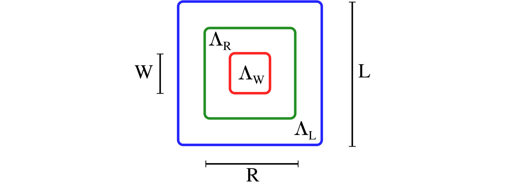 Figure 1
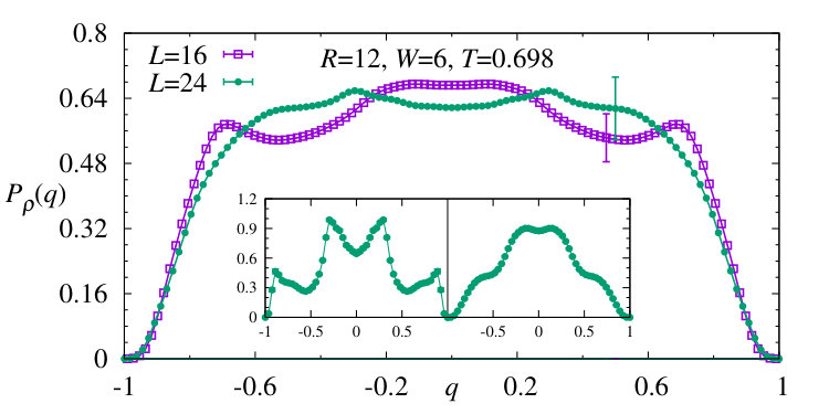 Figure 2
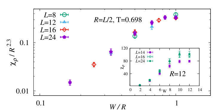 Figure 3
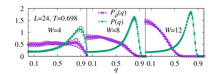 Figure 4
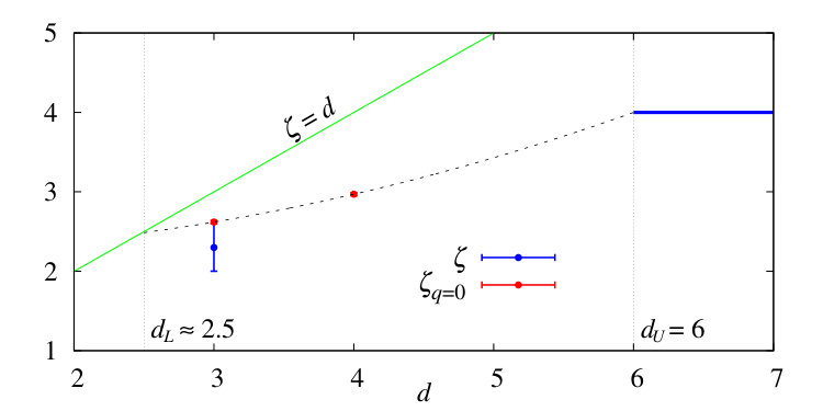 Figure 5
Peer Reviews
No public reviews on file for this paper yet. If you reviewed it on a platform where reviews are public (OpenReview, ICLR, NeurIPS, ICML), you can paste yours below so the community can read it here.
Videos
No videos yet. Explain this paper in a talk, walkthrough, or lecture? Add one.
Numerical construction of the Aizenman-Wehr metastate
A. Billoire
Institute de Physique Théorique, CEA Saclay and CNRS, 91191 Gif-sur-Yvette, France
L.A. Fernandez
Departamento de Física Teórica I, Universidad Complutense, 28040 Madrid, Spain
Instituto de Biocomputación y Física de Sistemas Complejos (BIFI), 50009 Zaragoza, Spain
A. Maiorano
Dipartimento di Fisica, Università di Roma La Sapienza, I-00185 Rome, Italy
Instituto de Biocomputación y Física de Sistemas Complejos (BIFI), 50009 Zaragoza, Spain
E. Marinari
Dipartimento di Fisica, Università di Roma La Sapienza, I-00185 Rome, Italy
Nanotec, Consiglio Nazionale delle Ricerche, I-00185 Rome, Italy
Istituto Nazionale di Fisica Nucleare, Sezione di Roma I, I-00185 Rome, Italy
V. Martin-Mayor
Departamento de Física Teórica I, Universidad Complutense, 28040 Madrid, Spain
Instituto de Biocomputación y Física de Sistemas Complejos (BIFI), 50009 Zaragoza, Spain
J. Moreno-Gordo
Departamento de Física Teórica I, Universidad Complutense, 28040 Madrid, Spain
Instituto de Biocomputación y Física de Sistemas Complejos (BIFI), 50009 Zaragoza, Spain
G. Parisi
Dipartimento di Fisica, Università di Roma La Sapienza, I-00185 Rome, Italy
Nanotec, Consiglio Nazionale delle Ricerche, I-00185 Rome, Italy
Istituto Nazionale di Fisica Nucleare, Sezione di Roma I, I-00185 Rome, Italy
F. Ricci-Tersenghi
Dipartimento di Fisica, Università di Roma La Sapienza, I-00185 Rome, Italy
Nanotec, Consiglio Nazionale delle Ricerche, I-00185 Rome, Italy
Istituto Nazionale di Fisica Nucleare, Sezione di Roma I, I-00185 Rome, Italy
J.J. Ruiz-Lorenzo
Departamento de Física and Instituto de Computación Científica Avanzada (ICCAEx), Universidad de Extremadura, 06071 Badajoz, Spain
Instituto de Biocomputación y Física de Sistemas Complejos (BIFI), 50009 Zaragoza, Spain
Abstract
Chaotic size dependence makes it extremely difficult to take the thermodynamic limit in disordered systems. Instead, the metastate, which is a distribution over thermodynamic states, might have a smooth limit. So far, studies of the metastate have been mostly mathematical. We present a numerical construction of the metastate for the Ising spin glass. We work in equilibrium, below the critical temperature. Leveraging recent rigorous results, our numerical analysis gives evidence for a dispersed metastate, supported on many thermodynamic states.
pacs:
75.10.Nr, 05.50.+q, 64.60.an
Introduction. Symmetry breaking and phase transitions are well defined for systems of infinite size, . Indeed, states can be defined rigorously as Dobrushin-Lanford-Ruelle (DLR) states ruelle:04 . However, experiments are conducted on systems of very large, but finite size. Therefore, one would like to interpret DLR states as the limit of states defined on a sequence of systems of growing size. Indeed, for simple systems, e.g. ferromagnets, we know how to approach DLR states with finite- states by using suitable boundary conditions. Yet, for disordered systems parisi:94 ; young:98 , the connection between DLR and finite- states is still much of a mistery AW-MS:90 , most particularly for spin-glasses NS ; NS-proc:03 ; NS-book:13 ; Arguin:11 ; Read:14 .
For the sake of concreteness, let us consider the standard model for spin-glasses, the Edwars-Anderson model EA:75 in spatial dimension . Ising spins , located in a size cube, (see Fig. 1), interact through a nearest neighbor, bond disordered and strongly frustrated Hamiltonian:
[TABLE]
The quenched couplings are independent and identically distributed random variables ( with probability, in our case). We call a disorder sample. The finite- Gibbs state is a random state, as it depends on the set of random couplings .
The problem in taking the large limit for spin-glasses defined by Eq. (1) is caused by their chaotic size-dependence. Take a fixed, arbitrary yet finite region (e.g. the measuring window in Fig. 1). The Gibbs measure over changes chaotically when the system grows by the addition of new couplings at the boundaries, while keeping previous couplings unaltered. This extreme sensibility to changes at the boundaries motivated the invention of the metastate NS , a probability distribution over states with a (hopefully) smoother limit.
The two main metastate definitions are Aizenman-Wehr’s AW-MS:90 and Newman-Stein’s NS . We shall focus on the former (the two definitions are conjectured to be equivalent NS-proc:03 , but the AW’s is easier to implement numerically). The lattice in Fig. 1 is divided into an inner region , a cube of linear size , and an outer region. Consequently we call internal couplings the set and outer couplings . We proceed by (i) restricting our attention to the measuring window of linear size Read:14 , (ii) taking the average over the outer couplings, with fixed internal couplings, and (iii) sending to infinity all three length scales while respecting . If the limit exists (which is yet to be proven), it is independent of the arbitrary choice for the fixed internal couplings 111For the sake of completeness, let us briefly recall the construction of the Newman-Stein metastate. In this approach, the set of couplings over the infinite lattice is fixed from the outset. A sequence of growing finite regions is considered, see Fig. 1 (all the cubes are centered at the origin of ). The Hamiltonians in Eq. (1) are truncated to the cube by a choice of boundary contitions (e.g. free boundary conditions). We consider the Gibbs state, as restricted to the measuring window . The Newman and Stein metastateNS records the frequency by which each state appears while the system size grows. The convergence of this sequence of states is yet to be proven. However, at least when the size of the measuring window gets large, the resulting metastate is expected to be independent of the initial choice of couplings (provide that this are typical)..
Yet, even if at a considerably lesser level of mathematical rigor, we must recall that there has been some progress in the study of spin glasses. We have numerical Palassini:99 ; Ballesteros:00 and experimental Gunnarson:91 evidences for the existence of a phase transition to a spin glass phase at low temperatures in , at least in the absence of an external magnetic field. We also have two major theoretical frameworks that are applied to interpret experiments and simulations: the replica symmetry breaking (RSB) theory MPV ; reviewJSP and the droplet model BM-Scaling1 ; BM-Scaling2 ; FH-DM . Which (if any) of these two theories captures the nature of the spin glass phase in is being debated Yucesoy-Billoire:12 .
In fact, a recent mathematical tour de force guerra ; talagrand ; panchenko has shown that the RSB theory provides the exact solution to the Sherrington-Kirkpatrick model sherrington:75 . The common lore expects RSB to be also valid above and at the upper critical dimension . RSB theory extends as well to features found in the mean field solution Parisi-RSB : many states (infinitely many in the limit), hierarchically organized, contribute to the Gibbs measure, each one with a weight that depends on the disorder realization. Consequences include the existence of de Almeida-Thouless line dealmeida:78 (the spin-glass phase transition survives in the presence of a small external magnetic field PNAS4d ), or the strong sample-to-sample fluctuations induced by the non-self-averageness of several measurable quantities Janus:11 (these observations PNAS4d ; Janus:11 were, however, obtained by simulating systems of finite size).
The alternative Droplet Model provides a much simpler scenario for the spin-glass phase, where the Gibbs measure is a mixture of two spin-flip related pure states. It follows that the spin-glass phase transition should disappear when a magnetic field is applied [the field breaks the global spin-flip symmetry in Eq. (1)].
The most recent mathematical analysis, based on metastates, has critically assessed both the RSB theory and the Droplet Model. Currently, we have three mathematically consistent pictures for the spin-glass phase. First, the Droplet Model metastate is concentrated on a single trivial state (let us call ‘trivial’ a state which is a mixture of two pure states related by the global spin-flip symmetry). Second, we have the Chaotic Pairs picture NS ; NS-book:13 , predicting a disperse metastate (there is a large number of states to choose from), yet each state is trivial. This non-trivial metastate is due to chaotic size-dependence: by gradually increasing , one obtains vastly different states. Finally, the RSB-metastate Read:14 is disperse and every state drawn from it contains the Parisi hierarchical tree of pure states. Alternatives to these three pictures are much limited by recent rigorous results Arguin:15 .
Read argues Read:14 that one can partially discriminate between these competing pictures for the metastate by studying the decay of a particular correlation function averaged over the metastate, for large distances , see Eq. (2). An exponent value implies a disperse metastate, thus ruling out the Droplet Model’s metastate. Furthermore, in the context of the RSB-metastate, the number of pure states that can be resolved by studying a region of size is exponentially large in .
To the best of our knowledge there has been only one numerical attempt to study the metastate, by means of a non-equilibrium simulation Young-MS . Yet, the main debated points regard the equilibrium metastate. In fact, the only related issue addressed numerically by equilibrium simulations has been non self-averageness Marinari:98 ; Janus:11 ; Yucesoy-Billoire:12 ; Middleton:13 ; Billoire:14 .
Here we show that a numerical construction of the Aizenman and Wehr metastate for the Edwards-Anderson model in is possible in present-day computers. Our construction makes precise several hints by Read Read:14 . In particular, recall Fig. 1, we show how big the ratios of lengthscales , need to be to uncover metastate properties. We also study the dependence on the fixed internal couplings, a crucial issue that hast not yet been addressed quantitatively. We make quantitative computations of overlap distributions and correlation functions averaged over the AW metastate, thus computing the crucial exponent. We find a value definitively smaller than , which rules out the Droplet Model metastate and leaves the Chaotic Pairs and the RSB metastates as the remaining contenders.
Metastate averages and the Metastate-averaged state. In the context depicted by Fig. 1, we consider model (1) endowed with periodic boundary contitions (which makes irrelevant the location of in ). Let us consider the probability distribution of at fixed internal disorder , while sending and averaging over the outer disorder :
[TABLE]
If the limit exists, it does not longer depend on the internal disorder and provides the AW metastate. The purpose of the “measuring window” in Fig. 1 is avoiding boundary effects, that may appear as long as is finite. Any measure is taken only inside , while bonds are fixed in in the metastate definition.
We have two kind of averages, thermal averages over the Gibbs state and averages over the metastate , that can be combined in different ways. For example, the metastate averaged state (MAS) is defined via the average .
As seen from the measuring window , a state is a set of probabilities over the spin configurations in . In other words, it is a point on the hyperplane defined by the equation , . In this sense, the metastate is a probability distribution over this hyperplane. The MAS is the average of this distribution, and it is itself a point on the hyperplane (hence, the MAS is a state itself).
The numerical construction of the metastate. We simulate the EA model () sampling spin configurations at equilibrium by a combination of Metropolis single spin flip Monte Carlo and Parallel Tempering PT . All the data shown are measured at the lowest simulated temperature , well below the critical temperature JANUS-crit:13 . Equilibration was assessed on a sample-by-sample basis JANUS:10 and, for the largest systems, it required the use of multi-site multi-spin coding (MUSI-MSC) fernandez:15 (see billoire:17 for details).
We repeat the computation for different internal couplings samples (indexed by ) and, for each of these, we use different outer disorder realizations (indexed by ) Thus we have a total of samples and, for each sample , we simulate distinct real replicas.
We take because we expect all inner disorder samples to be “typical” Read:14 when computing metastate averages at . We found however sizable sample to sample fluctuations for the system sizes we consider.
The average over the Gibbs state is estimated via Monte Carlo thermal averages at fixed disorder , i.e. for given indices and . The average over the metastate is given by , and the one over the internal disorder by . For example, the MAS spin correlation function is given by
[TABLE]
defining the Read’s exponent for .
We measure in the overlaps between any two real replicas — let us call it and — sharing the same internal disorder (indexed by ) and having external couplings indexed by and
[TABLE]
Actually, for each , we have contributions from different pairs of real replicas if and otherwise.
The main objects of our numerical study are the probability density functions (pdf) of the overlaps:
[TABLE]
While is the usual pdf already measured in many numerical simulation of spin glasses, is the pdf of the overlap over the MAS. Although for Read:14 , the scaling of its variance is informative
[TABLE]
Numerical results. Taking the limit of large in simulations actually amounts to asking how small the ratios and need to be, in order to find results which are safe (to a given accuracy).
In Fig. 2 (main plot) we see that that the MAS measured with and both and are statistically compatible, suggesting that is already a safe choice. The error bars are rather large, because the dependence of on the internal disorder sample is unexpectedly strong for the values of and we are using (as shown by the insets in Fig. 2).
A similar check can be performed with the MAS susceptibility (see Fig. 3). In the inset we see that, fixing , all data with are statistical compatible, while data with show significant deviations even for small values. Hereafter we safely fix .
The main panel of Fig. 3 shows data for the MAS susceptibility measured with the safe ratio (which is statistically equivalent to the limiting condition ) and different ratios . Data have been rescaled according to the following scaling law
[TABLE]
which is compatible with Eq. (4) if for and First of all we note that the physical behavior we would like to measure in the limit actually extends up to , where corrections to the asymptotic power law appear. Fitting data with we estimate Read’s exponent .
Finally we show in Fig. 4 the size dependence of both and , for (the largest simulated), and varying . For a dispersed metastate in the thermodynamic limit the two distributions are different.
Discussion and conclusions. We have shown that state-of-the-art numerical simulations of spin glasses in allow for the construction of the AW metastate. Numerical data suggest that the limiting conditions can be relaxed to without changing substantially the thermodynamic physical behavior. These are unexpected very good news.
From the numerical construction of the AW metastate we have obtained quantitative information on the nature of the spin glass phase in . The metastate average overlap distribution and the MAS are significantly distinct objects already at moderate sizes. We cannot extrapolate safely to the thermodynamic limit, and sample to sample fluctuations are still important at the accessible system sizes. Nevertheless we have found a convincing scaling law for the MAS susceptibility, and an estimate of , strongly suggesting .
Read’s exponent is related to the number of different states that can be measured in a system of size as Read:14 . Such a number diverges in the thermodynamic limit as long as , supporting the picture of a metastate with infinitely many states. In Fig. 5 we summarize our knowledge about the exponent. At and above the upper critical dimension , where mean field exponents are correct, DD:99 ; RFSGBook . Assuming is a continuous and monotonically non-decreasing function, the inequality still holds slightly below . In the present work we find (blue point in Fig. 5). An alternative estimate of the exponent comes from the decay of the 4-spins spatial correlation function conditional to the sector, for : JANUS:09 ; JANUS:10 ; UNPUB and NICOLAO:14 . Read conjectured that Read:14 . These estimates are shown by red points in Fig. 5 222The conjectured relation RFSGBook , where is the anomalous dimension at the critical point, does not work in JANUS:09 ; JANUS:10 ; UNPUB ; NICOLAO:14 .. A gentle interpolation of the estimates (dashed line in Fig. 5) seems to meet the condition very close to the current best estimate for the lower critical dimension Boettcher .
In conclusions, all the numerical evidences strongly support the existence of a spin glass metastate dispersed over infinitely many states for (and probably down to the lower critical dimension). These findings are incompatible with the Droplet Model, while are compatible with both the Chaotic Pais picture and the Replica Symmetry Breaking scenario.
I Acknowledgments
This project has received funding from the European Research Council (ERC) under the European Union’s Horizon 2020 research and innovation program (grant agreement No 694925). We were partially supported by MINECO (Spain) through Grant Nos. FIS2012-35719-C02-01, FIS2013-42840-P, FIS2015-65078-C2, FIS2016-76359-P (contract partially funded by FEDER), and by the Junta de Extremadura (Spain) through Grant No. GRU10158 (partially funded by FEDER). Our simulations were carried out at the BIFI supercomputing center (using the Memento and Cierzo clusters), at the TGCC supercomputing center in Bruyères-le-Châtel (using the Curie computer, under the allocation 2015-056870 made by GENCI) and at ICCAEx supercomputer center in Badajoz (GrInFishpc and ICCAExhpc). We thank the staff at BIFI, TGCC and ICCAEx supercomputing centers for their assistance.
The reference list from the paper itself. Each links out to its DOI / PubMed record.
- 1(1) D. Ruelle, Thermodynamic Formalism: The Mathematical Structures of Equilibrium Statistical Mechanics , 2nd Ed. (Cambridge University Press, Cambridge, 2004).
- 2(2) G. Parisi, Field Theory, Disorder and Simulations , (World Scientific, Singapore, 1994).
- 3(3) A. P. Young, Spin Glasses and Random Fields , (World Scientific, Singapore, 1998).
- 4(4) M. Aizenmann and J. Wehr, Comm. Math. Phys. 130 , 489 (1990).
- 5(5) C. M. Newman and D. L. Stein, Phys. Rev. B 46 , 973 (1992); Phys. Rev. Lett. 76 , 4821 (1996); Phys. Rev. E 55 , 5194 (1997); Phys. Rev. E 57 , 1356 (1998).
- 6(6) C. M. Newman and D. L. Stein, in Mathematics of Spin Glasses and Neural Networks , ed. A. Bovier and P. Picco (Birkhauser, Boston 1997); J. Phys.: Condens. Matter 15 , R 1319 (2003).
- 7(7) D. L. Stein, and C. M. Newman, Spin Glasses and Complexity (Princeton University Press, 2013).
- 8(8) L. P. Arguin and M. Damron, J. Stat. Phys. 143 , 226 (2011).