
TL;DR
This paper investigates the asymptotic behavior of the perimeter and area of convex hulls of planar random walks, establishing variance limits and distributional convergence, including non-Gaussian limits, for different drift conditions.
Contribution
It provides new variance limit results and distributional limit theorems for convex hull metrics of planar random walks, extending previous work to non-Gaussian limits.
Findings
Variance of perimeter length converges after normalization.
Central limit theorem established for perimeter length.
Non-Gaussian distributional limits identified for convex hull metrics.
Abstract
For the perimeter length and the area of the convex hull of the first steps of a planar random walk, this thesis study mean and variance asymptotics and establish distributional limits. The results apply to random walks both with drift (the mean of random walk increments) and with no drift under mild moments assumptions on the increments. Assuming increments of the random walk have finite second moment and non-zero mean, Snyder and Steele showed that converges almost surely to a deterministic limit, and proved an upper bound on the variance Var. We show that Var converges and give a simple expression for the limit, which is non-zero for walks outside a certain degenerate class. This answers a question of Snyder and Steele. Furthermore, we prove a central limit theorem for in the non-degenerate case. Then…
Click any figure to enlarge with its caption.
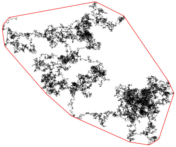 Figure 1
 Figure 2
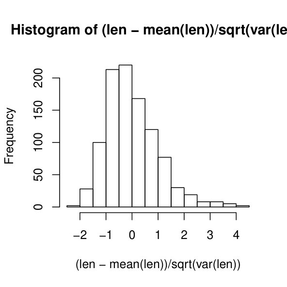 Figure 3
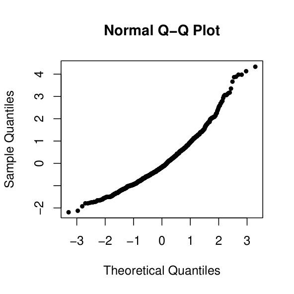 Figure 4
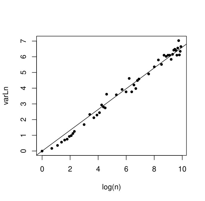 Figure 5
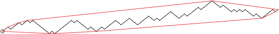 Figure 6
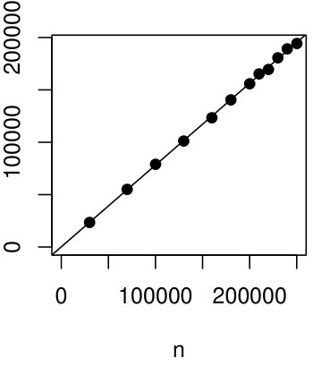 Figure 7
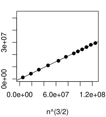 Figure 8
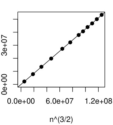 Figure 9
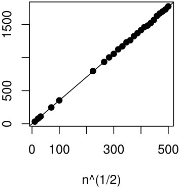 Figure 10
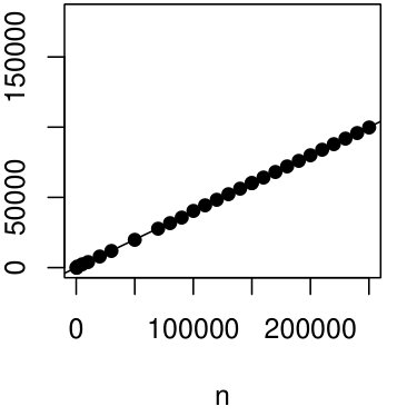 Figure 11
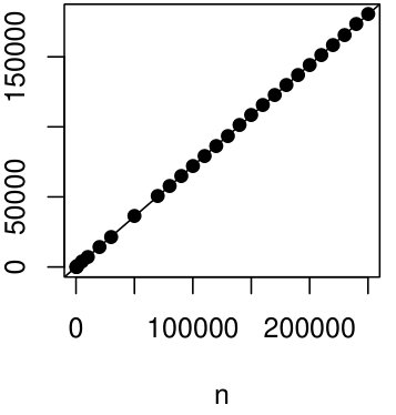 Figure 12
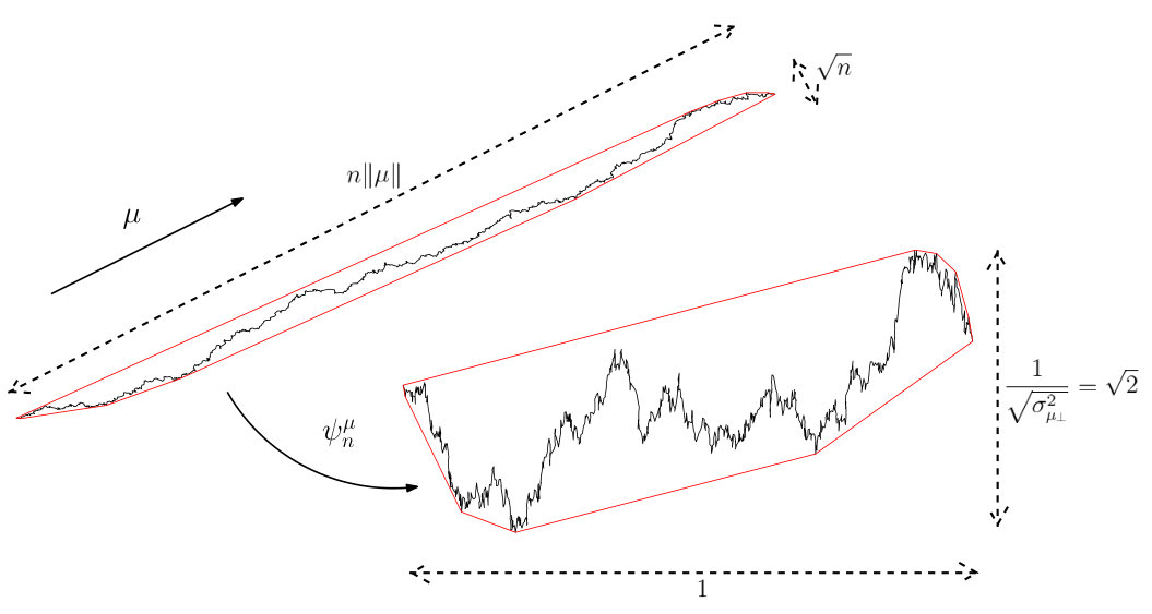 Figure 2
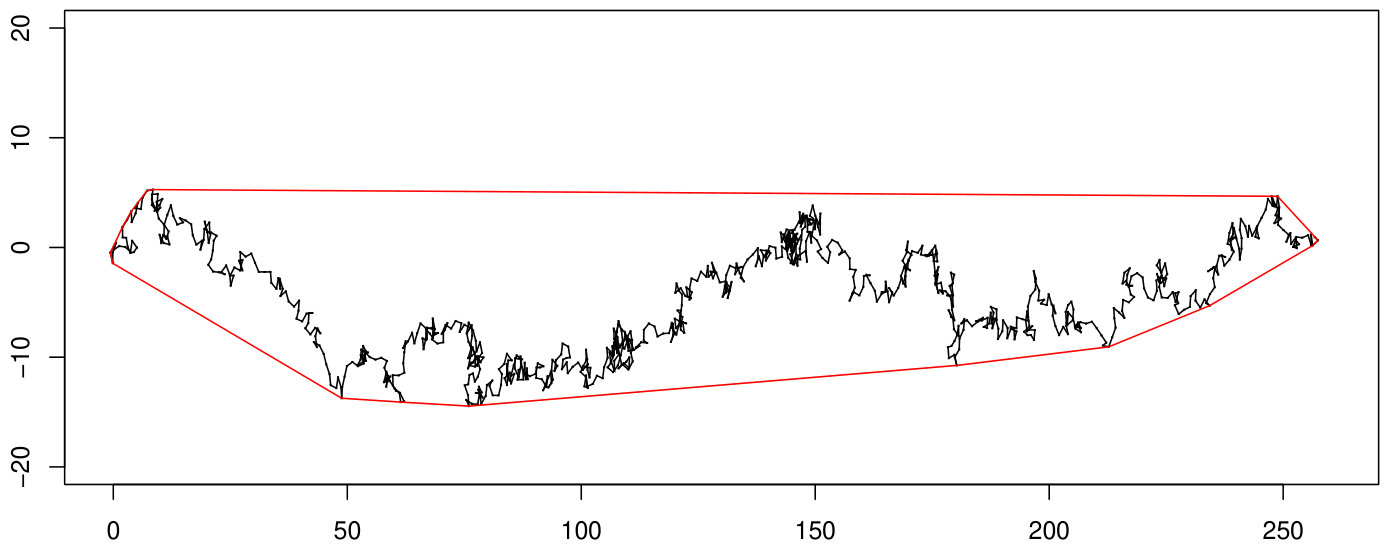 Figure 14
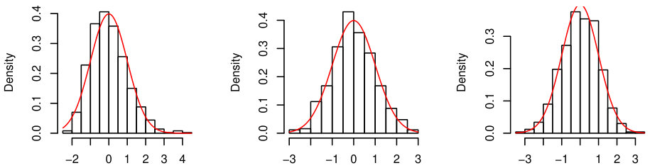 Figure 15
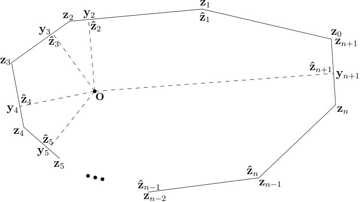 Figure 16
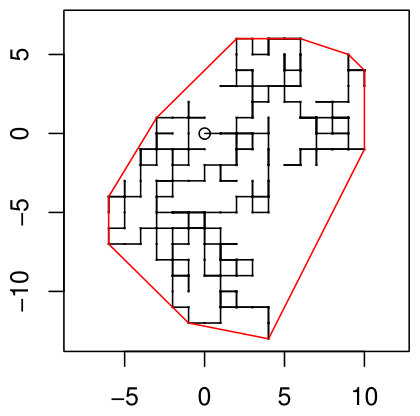 Figure 17
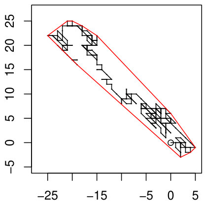 Figure 18
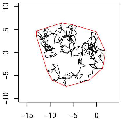 Figure 19
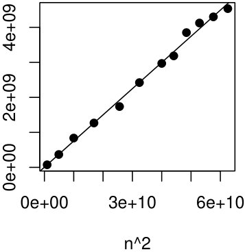 Figure 20
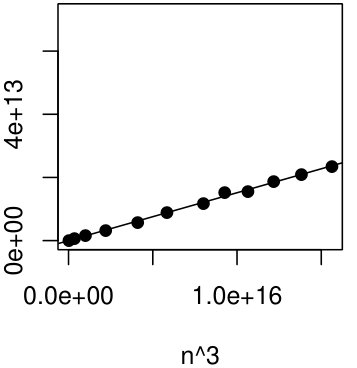 Figure 21
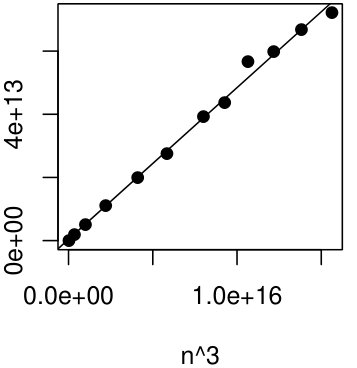 Figure 22
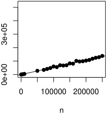 Figure 23
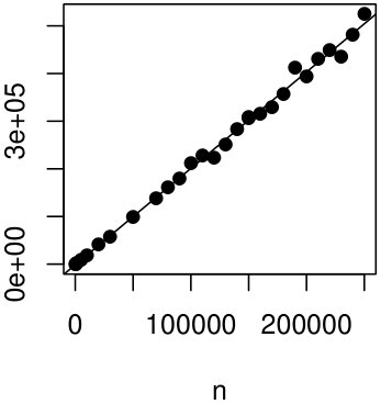 Figure 24
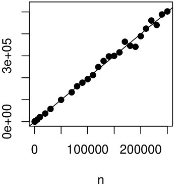 Figure 25
| Page | |||
| , | : | random walk with location and increments | 1.1 |
| : | the convex hull of random walk | 1.5 | |
| : | the random walk | 3.1 | |
| : | the perimeter length of | 1.5 | |
| : | the area of | 1.5 | |
| : | the Euclidean norm | 1.5 | |
| : | the mean drift vector | 1.1 | |
| : | the covariance matrix associated with | 1.1 | |
| : | the matrix square-root of | 3.3 | |
| : | 1.1 | ||
| : | for | 1.5 | |
| : | 1.5 | ||
| : | 1.1 | ||
| : | the class of continuous functions from to | 2.7 | |
| : | 2.7 | ||
| : | the supremum metric | 2.7 | |
| : | for and a point | 2.7 | |
| : | 2.7 | ||
| : | 2.7 | ||
| : | , the unit sphere in | 2.7 | |
| : | the collection of convex compact sets in | 2.7 | |
| : | 2.7 | ||
| : | the Hausdorff metric | 2.7 | |
| : | the parallel body at distance | 2.7 | |
| : | , standard Brownian motion in | 2.8 | |
| : | the area of convex compact sets in the plane | 2.9 | |
| : | the perimeter length of convex compact sets | 2.9 | |
| : | the support function of | 2.7 | |
| : | for | 3.2 | |
| : | the convex hull of the Brownian path up to time | 3.4 | |
| : | 3.5 | ||
| : | 3.5 | ||
| : | weak convergence | 2.26 | |
| : | , standard Brownian motion in | 3.1 | |
| : | , for | 3.3 | |
| : | 3.3 | ||
| : | 3.3 | ||
| : | the indicator function | 4.2 | |
| : | 4.2 | ||
| : | 4.2 | ||
| : | 5.26 | ||
| , | : | defined in equation (6.1) | 6.1 |
| lower bound | simulation estimate | upper bound | |
|---|---|---|---|
| 1.08 | 9.87 |
| lower bound | simulation estimate | upper bound | |
|---|---|---|---|
| 0.30 | 5.22 | ||
| 0.019 | 2.08 |
| limit exists for | limit exists for | limit law | ||
|---|---|---|---|---|
| § | non-Gaussian | |||
| ¶ | non-Gaussian | |||
| §† | ‡ | Gaussian‡ | ||
| non-Gaussian |
| lower bound | simulation estimate | upper bound | |
|---|---|---|---|
| 1.08 | 9.87 | ||
| 0.30 | 5.22 | ||
| 0.019 | 2.08 |
Peer Reviews
No public reviews on file for this paper yet. If you reviewed it on a platform where reviews are public (OpenReview, ICLR, NeurIPS, ICML), you can paste yours below so the community can read it here.
Videos
No videos yet. Explain this paper in a talk, walkthrough, or lecture? Add one.
Taxonomy
TopicsDiffusion and Search Dynamics · Point processes and geometric inequalities · Stochastic processes and statistical mechanics
Convex Hulls of Planar Random Walks
3rd March 2024
Chang Xu
Department of Mathematics and Statistics
University of Strathclyde
Glasgow, UK
This thesis is submitted to the University of Strathclyde for the
degree of Doctor of Philosophy in the Faculty of Science.
The copyright of this thesis belongs to the author under the terms of the United Kingdom Copyright Acts as qualified by University of Strathclyde Regulation 3.50. Due acknowledgement must always be made of the use of any material in, or derived from, this thesis.
Acknowledgements
My deepest gratitude goes to my supervisor Doctor Andrew Wade and Professor Xuerong Mao. This thesis would not exist without their constant support.
I also need to thank Prof. Mikhail Menshikov at Durham University, my current and former colleagues Andreas Wachtel, Dr. Hongrui Wang, Dr. Wei Liu, Dr. Jiafeng Pan et al. for plenty of valuable advice and help during my PhD study.
Last, I would like to express my thanks to my family and the University of Strathclyde for the financial support.
Abstract
For the perimeter length and the area of the convex hull of the first steps of a planar random walk, this thesis study mean and variance asymptotics and establish distributional limits. The results apply to random walks both with drift (the mean of random walk increments) and with no drift under mild moments assumptions on the increments.
Assuming increments of the random walk have finite second moment and non-zero mean, Snyder and Steele showed that converges almost surely to a deterministic limit, and proved an upper bound on the variance . We show that converges and give a simple expression for the limit, which is non-zero for walks outside a certain degenerate class. This answers a question of Snyder and Steele. Furthermore, we prove a central limit theorem for in the non-degenerate case.
Then we focus on the perimeter length with no drift and area with both drift and zero-drift cases. These results complement and contrast with previous work and establish non-Gaussian distributional limits. We deduce these results from weak convergence statements for the convex hulls of random walks to scaling limits defined in terms of convex hulls of certain Brownian motions. We give bounds that confirm that the limiting variances in our results are non-zero.
Contents
-
4 Spitzer–Widom formula for the expected perimeter length and its consequences
-
6.2 Upper bound for the expected value and variance for the area
Notations
Chapter 1 Introduction
1.1 Background on Random Walk
Let be independent identically distributed (i.i.d.) random variables taking values in and let . is a random walk [30, p. 88].
Random walk theory is a classical and well-studied topic in probability theory. In 1905, Albert Einstein studied the Brownian motion in his paper “On the Movement of Small Particles Suspended in a Stationary Liquid Demanded by the Molecular-Kinetic Theory of Heat”. Brownian motion is the random motion of particles in a fluid which is found by the botanist Robert Brown in 1827 [32, Sec. 2.1]. He noted that the pollen grains in water kept moved through randomly. Einstein explained in details how the motion that Brown had observed was a result of the pollen being moved by individual water molecules.
Scientists then gave the mathematical formalisation for the Brownian motion and its generalisation: random walk. The term random walk was first used by Karl Pearson in 1905. In a letter to Nature, he gave a simple model to describe a mosquito infestation in a forest. At each time step, a single mosquito moves a fixed length in a randomly chosen direction. Pearson wanted to know the distribution of the mosquitoes after many steps had been taken. The letter was answered by Lord Rayleigh, who had already solved a more general form of this problem in 1880, in the context of sound waves in heterogeneous materials. Modelling a sound wave travelling through the material can be thought of as summing up a sequence of random wave-vectors of constant amplitude but random phase since sound waves in the material have roughly constant wavelength, but their directions are altered at scattering sites within the material.
There are some classical results we need to bear in mind when we study random walks. First we need to introduce the concepts of recurrence and transience. A random walk taking values in is called point-recurrent if
[TABLE]
and point-transient if
[TABLE]
If the random walk is not discrete then these definitions are not very useful. Instead we say that the random walk is neighbourhood-recurrent if for some ,
[TABLE]
and neighbourhood-transient if
[TABLE]
In the discrete case, for a simple random walk we have the Pólya’s theorem [48]. A random walk on is simple if for any ,
[TABLE]
Theorem 1.1** (Pólya).**
A simple random walk in is recurrent for or and transient for .
This theorem was generalised by Chung and Fuchs [15] in 1951.
Theorem 1.2** (Chung–Fuchs).**
Let be a random walk in . Then,
- (i)
If and in probability, then is neighbourhood-recurrent. 2. (ii)
If and converges in distribution to a centred normal distribution, then is neighbourhood-recurrent. 3. (iii)
If and the random walk is not contained in a lower-dimensional subspace, then it is neighbourhood-transient.
1.2 Background on geometric probability
A central theme of classical geometric probability or stochastic geometry concerns the study of the properties of random point sets in Euclidean space and associated structures. For example, a large literature is devoted to study of the lengths of graphs on random vertex sets in Euclidean space , . The interests are primarily in the lengths of those graphs representing the solutions to problems in Euclidean combinatorial optimization (see [60] or [67]). In the classical setting, the random point sets are generated by i.i.d. random variables. Some typical problems involve the construction of the shortest possible network of some kind:
Let be i.i.d. random points with common distribution on and .
- (i)
Travelling salesman problem. Find the length of shortest closed path traversing each vertex in exactly once. 2. (ii)
Minimal spanning tree. Find the minimal total edge length of a spanning tree through . 3. (iii)
Minimal Euclidean matching. Find the minimal total edge length of a Euclidean matching of points in .
Many of the questions of geometric probability or stochastic geometry are equally valid for point sets generated by random walk trajectories.
1.3 Random convex hulls
We first define the convex hull here. A set in is convex if it has the following property [29, p. 42]:
[TABLE]
Given a set in , its convex hull is the intersection of all convex sets in which contain . Since the intersection of convex sets is always convex, the convex hull of is convex and it is the smallest convex set in with respect to set inclusion, which contains .
One of the motivations to study the convex hulls is to find the extreme values in the random points. For the 1-dimensional case, the extreme values are just the maximum and minimum values. For higher dimensional cases, the extreme values could be determined by the convex hulls.
However, the extreme values have different meanings in these two different main settings of classical stochastic geometry. For the setting of i.i.d. random points, one important concern is the outlier detection in random sample. For the setting of trajectories of stochastic processes, extremes are important for study of record values. It gives two related but different streams of research, with different underlying probabilistic models and different motivating questions, though generally the motivations are all comes from multidimensional theory of extremes. See for example [4], [5], [6] and [45].
1.3.1 i.i.d. random points
Convex hulls of iid. random points, also known as random polytopes, were first studied by Geffroy [24] (1961), Rényi and Sulanke [50] (1963), and Efron [18] (1965). In the case where the points are normally distributed, the resulting convex hulls are known as Gaussian polytopes. See Reitzner [49, Random polytopes, pp. 45-76] (2010) and Hug [31] (2013) for recent surveys.
Motivation arises in statistics (multivariate extremes) and convex geometry (approximation of convex sets), and there are connection to the isotropic constant in functional analysis: see Reitzner [49]. He also listed some other applications including to the analysis of algorithms and optimization.
For the multivariate extremes, let be the iid. random points with common distribution on and . In the case of , iid. points extremes are used in outlier detection in statistics. In the case of , Green [28] describes the peeling algorithm for detection of multivariate outliers via the iterated removal of points on the boundary of the convex hulls.
For the approximation of convex sets, Reitzner [49] insulates the algorithms to efficiently compute convex hull for large point set in .
1.3.2 Trajectories of stochastic process
Before the study of random polytopes, Lévy [40] had considered the convex hull of planar Brownian motion. The study of convex hull of random walk goes back to Spitzer and Widom [58]. Generally, the convex hull of a stochastic process is an interesting geometrical object, related to extremes of the stochastic processes, giving a multivariate analogue of record values.
In one dimension, a value of a process is a record value if it is either less than all previous values (a lower record) or greater than all previous values (an upper record). In higher dimensions, a natural definition of “record” is then a point that lies outside the convex hull of all previous values.
More recent work on convex hull of Brownian motion includes Burdzy [11] (1985), Cranston, Hsu and March [13] (1989), Eldan [20] (2014), Evans [21] (1985), Pitman and Ross [47] (2012).
For general stochastic processes, convex hulls and related convex minorants or majorants, are studied by Bass [8] (1982) and Sinai [55] (1998).
1.4 Applications for convex hulls of random walks
In recent studies of random walks, attention has focussed on various geometrical aspects of random walk trajectories. Many of the questions of stochastic geometry, traditionally concerned with functionals of independent random points, are also of interest for point sets generated by random walks.
Study of the convex hull of planar random walk goes back to Spitzer and Widom [58] and the continuum analogue, convex hull of planar Brownian motion, to Lévy [40, §52.6, pp. 254–256]; both have received renewed interest recently, in part motivated by applications arising for example in modelling the ‘home range’ of animals. Random walks have been extensively used to model the movement of animals; Karl Pearson’s original motivation for the random walk problem originated with modelling the migration of animal species such as mosquitoes, and subsequently random walks have been used to model the locomotion of microbes: see [16, 56] for surveys. If the trajectory of the random walker represents the locations visited by a roaming animal, then the convex hull is a natural estimate of the ‘home range’ of the animal [65, 66]. Natural properties of interest are the perimeter length and area of the convex hull. See [42] for a recent survey of motivation and previous work. The method of Chapter 3 in part relies on an analysis of scaling limits, and thus links the discrete and continuum settings.
1.5 Introduction of the model
On each unsteady step, a drunken gardener deposits one of seeds. Once the flowers have bloomed, what is the minimum length of fencing required to enclose the garden?
Let be a sequence of independent, identically distributed (i.i.d.) random vectors on . Write for the origin in . Define the random walk by and for , . Let be the convex hull of positions of the walk up to and including the th step, which is the smallest convex set that contains . Let denote the length of the perimeter of and be the area of the convex hull. (See Figure 1.1.)
We will impose a moments condition of the following form:
(Mp)
Suppose that .
For almost everything that follows, we will assume that at least the case of ((Mp)) holds, and frequently we will assume the case. For several of our results we assume that ((Mp)) holds for some . In any case, we will be explicit about which case we assume at any particular point.
Given that ((Mp)) holds for some , then , the mean drift vector of the walk, is well defined. If ((Mp)) holds for some , then \Sigma:=\mathbb{E}\,[(Z_{1}-\mu)(Z_{1}-\mu)^{\scalebox{0.6}{\top}}], the covariance matrix associated with , is well defined; is positive semidefinite and symmetric. We write . Here and elsewhere and are viewed as column vectors, and \|\mkern 1.5mu\raisebox{1.7pt}{\scalebox{0.4}{\bullet}}\mkern 1.5mu\| is the Euclidean norm. We also introduce the decomposition \sigma^{2}=\sigma^{2}_{\mu}+\sigma^{2}_{\mu_{\mkern-1.0mu\scalebox{0.5}{\perp}}} with
[TABLE]
Here and elsewhere, ‘’ denotes the scalar product, for , and .
Convex hulls of random points have received much attention over the last several decades: see [42] for an extensive survey, including more than 150 bibliographic references, and sources of motivation more serious than our drunken gardener, such as modelling the ‘home-range’ of animal populations. An important tool in the study of random convex hulls is provided by a result of Cauchy in classical convex geometry. Spitzer and Widom [58], using Cauchy’s formula, and later Baxter [9], using a combinatorial argument, showed that
[TABLE]
Note that thus scales like in the case where the one-step mean drift vector but like in the case where (provided ). The Spitzer–Widdom–Baxter result, in common with much of the literature, is concerned with first-order properties of : see [42] for a summary of results in this direction for various random convex hulls, with a specific focus on (driftless) planar Brownian motion.
Much less is known about higher-order properties of . There is a clear distinction between the zero drift case () and the non-zero drift case (). For example, denote . Note that is non decreasing in , because . We investigated the asymptotic behaviour of in the following two different cases.
Proposition 1.3**.**
- (i)
Suppose and . Then a.s. 2. (ii)
Suppose and . Then a.s.
Proof.
- (i)
In the first case, the random walk () is recurrent (see e.g. [17]). There exists , depending on the distributioon of , such that will visit any ball of radius at least infinitely often (e.g., in the case of simple symmetric random walk on , it suffices to take ). Let . Then, will visit infinitely often for each . Here the notation is a Euclidean ball (a disk) with centre and radius .
So there exists some random time with a.s. such that contains a point in each of these four balls, and so contains the square with these points as its corners, which in turn contains . So for any . So . 2. (ii)
In the second case, the random walk is transient (see [17]). Let be a wedge with apex with a angle (say ) so that is bisected by . By the Strong Law of Large Numbers, and so , where is the normal vector of . This implies the number of points outside the wedge is finite for any . We take some inside the wedge and denote the set of finitely many points outside by . Note that is outside so the set is non-empty. Hence, there must be some standing on the boundary of the convex hull, for all . Then, , which implies a.s. since is non decreasing.
∎
Remark 1.1*.*
The key property for (i) is not (compact set) recurrence, but angular recurrence in the sense that visits any cone with apex at and non-zero angle infinitely often. Thus the same distinction between (i) and (ii) persists for random walks in , , with the notation extended in the natural way.
Because of this distinction, we always separate the arguments of and into the cases of non-zero and zero drift.
To illustrate our model, here we give some pictures of simulation examples (see Figure 1.3).
1.6 Outline of the thesis
Chapter 2 is some necessary mathematical prerequisites for our results. It includes the concepts of the study objects and the essential tools used in the rest chapters.
In Chapter 3 we describe our scaling limit approach, and carry it through after presenting the necessary preliminaries; the main new results of this chapter, Theorems 3.6 and 3.8, give weak convergence statements for convex hulls of random walks in the case of zero and non-zero drift, respectively. Armed with these weak convergence results, we present asymptotics for expectations and variances of the quantities and in Section 5.4, 6.4 and 6.5; the arguments in this section rely in part on the scaling limit apparatus, and in part on direct random walk computations. This section concludes with upper and lower bounds we found for the limiting variances.
Snyder and Steele [57] showed that converges almost surely to a deterministic limit, and proved an upper bound on the variance [57]. In Chapter 4, we give a different approach to prove their major results, which includes the fact that converges (Proposition 4.7) and a simple expression for the limit in Proposition 4.5. For the zero drift case, we give a new improved limit expression in Proposition 4.9.
Chapter 5 gives the convergence of in Proposition 5.4, which is first proved by Snyder and Steele [57]. They also gave the law of large numbers for in the non-zero drift case. But we found it also valid for the zero drift case (Proposition 5.5). Apart from that, the following of major results in this chapter are new. For the non-zero drift case, we give a simple expression for the limit of in Theorem 5.13 [63, Theorem 1.1], which is non-zero for walks outside a certain degenerate class. This answers a question of Snyder and Steele. It is also the only case where the perimeter length is Gaussian. So we give a central limit theorem for in this case in Theorem 5.14 [63, Theorem 1.2]. For the non-zero drift case, the limit expression of is given in Proposition 5.15 [64, Proposition 3.5] and its upper and lower bounds are given by Proposition 5.16 [64, Proposition 3.7].
Chapter 6 is an analogue of Chapter 5 for the area . In Theorem 6.8 we give the asymptotic for the expected area with zero drift, which is a bit more general than the form given by Barndorff–Nielsen and Baxter [3]. Apart from that, the following of major results in this chapter are new. We give the asymptotic for the expected area with drift in Proposition 6.9 [64, Proposition 3.4] and also the asymptotics for their variance in both zero drift (Proposition 6.12 [64, Proposition 3.5]) and non-zero drift cases (Proposition 6.13 [64, Proposition 3.6]). Meanwhile, some upper and lower variance bounds are provided by the last section of this chapter.
Chapter 2 Mathematical prerequisites
2.1 Convergence of random variables
First of all, we define the different modes of convergence we will need in this thesis.
Let and be random variables in .
converges almost surely to () as iff
[TABLE]
converges in probability to () as iff, for every ,
[TABLE]
The norm of is defined by
[TABLE]
converges in to () for , as iff
[TABLE]
Let , be the distribution function of and let be the continuity set of . converges in distribution to () as iff
[TABLE]
The concept of convergence in distribution extends to random variables in in terms of the joint distribution functions .
These modes of convergence have the following logical relationships.
[TABLE]
Now we collect some basic results on deducing convergence lemmas and theorems.
Lemma 2.1** (Dominated convergence [30] p.57).**
Let and be random variables. Suppose that for all , where , and that a.s. as . Then
[TABLE]
In particular,
[TABLE]
Lemma 2.2** (Pratt’s lemma [30] p.221).**
Let and be random variables. Suppose that almost surely as , and that
[TABLE]
Then
[TABLE]
Lemma 2.3** (The Borel–Cantelli lemma [30] p.96, 98).**
Let be arbitrary events. Then
[TABLE]
Moreover, suppose that are random variables. Then,
[TABLE]
Lemma 2.4** (Slutsky’s theorem [30] p.249).**
Let and be sequences of random variables, Suppose that
[TABLE]
where is some constant. Then,
[TABLE]
Here we also introduce some useful concepts of uniform integrability.
A collection of random variables , , is said to be uniformly integrable if
[TABLE]
Lemma 2.5**.**
Let and be random variables. If in probability then the following are equivalent:
- (i)
* is uniformly integrable.* 2. (ii)
* in .* 3. (iii)
.
Lemma 2.6** (convergence of means [35] p.45).**
Let be -valued random variables with . If is uniformly integrable, then as .
2.2 Martingales
A sequence of random variables is -adapted if is -measurable for all , which means for any , .
An integrable {}-adapted sequence is called a martingale if
[TABLE]
It is called a submartingale if
[TABLE]
and a supermartingale if
[TABLE]
An integrable, {}-adapted sequence {} is called a martingale difference sequence if
[TABLE]
Then, the sequence of is -martingale since
[TABLE]
which indicate
[TABLE]
Lemma 2.7** (Orthogonality of martingale differences [30] p.488).**
Let be a martingale difference sequence. Then for . Hence,
[TABLE]
We use a standard martingale difference construction based on resampling. Consider the functional on , . Let be iid. random variables and . Let be independent copies of and
[TABLE]
Let where .
Lemma 2.8**.**
Let . Then
- (i)
; 2. (ii)
* whenever the latter sum is finite.*
Proof.
The idea is well known. Since is independent of ,
[TABLE]
So,
[TABLE]
Hence is martingale differences, since
[TABLE]
and
[TABLE]
So,
[TABLE]
But by orthogonality of martingale differences, (Lemma 2.7),
[TABLE]
∎
Note that by the conditional Jensen’s inequality , we have
[TABLE]
So from part (ii) of Lemma 2.8,
[TABLE]
This gives a upper bound for the variance of , which is a factor of larger than the upper bound obtained from the Efron–Stein inequality (equation (2.3) in [57]):
Lemma 2.9**.**
[TABLE]
2.3 Reflection principle for Brownian motion
Lemma 2.10** (Reflection principle [44] p.44).**
If is a stopping time and is a standard 1-dimensional Brownian motion, then the process called Brownian motion reflected at and defined by
[TABLE]
is also a standard Brownian motion.
Corollary 2.11**.**
Suppose and is a standard 1-dimensional Brownian motion. Then,
[TABLE]
2.4 Useful inequalities
We collect some useful inequalities which is useful in the next chapters.
Lemma 2.12** (Markov’s inequality [30] p.120).**
Let be a random variable. Suppose that for some , and let . Then,
[TABLE]
Lemma 2.13** (Chebyshev’s inequality [30] p.121).**
Let be a random variable. Suppose that . Then for ,
[TABLE]
Lemma 2.14** (The Cauchy–Schwarz inequality [30] p.130).**
Suppose that random variables and have finite variances. Then,
[TABLE]
The next result generalises the Cauchy–Schwarz inequality.
Lemma 2.15** (The Hölder inequality [30] p.129).**
Let and be random variables. Suppose that , and , then
[TABLE]
Lemma 2.16** (The Minkowski inequality [30] p.129).**
Let . Suppose that and are random variables, such that and . Then,
[TABLE]
This is the triangle inequality for the norm.
Now we introduce some inequalities on martingales.
Lemma 2.17** (Doob’s inequality [17] p.214).**
If is a martingale, then for ,
[TABLE]
Lemma 2.18** (Azuma–Hoeffding inequality [46] p.33).**
Let be a martingale difference sequence adapted to a filtration , which means is -measurable and . Then, for any ,
[TABLE]
where is such that a.s. for all .
We also introduce some inequalities for sums of independent random variables.
Lemma 2.19** (Marcinkiewicz–Zygmund inequality [30] p.151).**
Let . Suppose that are independent, identically distributed random variables with mean 0 and . Set . Then there exists a constant depending only on , such that
[TABLE]
Lemma 2.20** (Rosenthal’s inequality [30] p.151).**
Let . Suppose that are independent random variables such that for all . Set . Then,
[TABLE]
2.5 Useful theorems and lemmas
Lemma 2.21** (Fubini’s theorem [30] p.65).**
Let () and () be probability spaces, and consider the product space (), where is the product measure. Suppose that is a two-dimensional random variable, and that is -measurable, and (i) non-negative or (ii) integrable. Then,
[TABLE]
Lemma 2.22**.**
Let be a sequence of real numbers and let . If as , then as .
Proof.
By assumption, for any there exists such that for all . Then,
[TABLE]
for all big enough. Since was arbitrary, the result follows. ∎
2.6 Multivariate normal distribution
Let be a symmetric positive semi-definite () matrix. Then, there exists an unique positive semi-definite symmetric matrix such that [41]. The matrix can also be regarded as a linear transform of given by .
For a random variable , the notation means has dimensional normal distribution with mean [math] and covariance matrix . In the degenerate case, all entries of the covariance matrix is [math], , which means that almost surely.
Lemma 2.23**.**
Suppose and let . Then .
Lemma 2.24** (Multidimensional Central Limit Theorem [41] p.62).**
Suppose is a sequence of i.i.d. random variables on . is a random walk on . If , and , then
[TABLE]
2.7 Analytic and Geometric prerequisites
We recall a few basic facts from real analysis: [53] is an excellent general reference. The Heine–Borel theorem states that a set in is compact if and only if it is closed and bounded [53, p. 40]. Compactness is preserved under continuous mappings: if is a compact metric space and is a metric space, and is continuous, then the image is compact [53, p. 89]; moreover is uniformly continuous on [53, p. 91]. For any such uniformly continuous , there is a monotonic modulus of continuity such that for all , and for which as (see e.g. [35, p. 57]).
Let be a positive integer. For , let denote the class of continuous functions from to . Endow with the supremum metric
[TABLE]
Let denote those functions in that map [math] to the origin in .
Usually, we work with , in which case we write simply
[TABLE]
For and , define , the image of under . Note that, since is compact and is continuous, the interval image is compact. We view elements as paths indexed by time , so that is the section of the path up to time .
We need some notation and concepts from convex geometry: we found [29] to be very useful, supplemented by [58] as a convenient reference for a little integral geometry. Let be a positive integer. Let denote the Euclidean distance between and in . For a set , write for the boundary of (the intersection of the closure of with the closure of ), and for the interior of . For and a point , set , with the usual convention that . We write for Lebesgue measure on . Write for the unit sphere in .
Let denote the collection of convex compact sets in , and write
[TABLE]
for those sets in that include the origin. The Hausdorff metric on will be denoted
[TABLE]
Given , for set
[TABLE]
the parallel body of at distance . Note that, two equivalent descriptions of (see e.g. Proposition 6.3 of [29]) are for ,
[TABLE]
where is the support function of and is the inner product of and , i.e. .
2.8 Continuous mapping theorem and Donsker’s Theorem
We consider random walks in in this section. First we need to define the weak convergence in .
Suppose is a probability space and is a metric space. For , suppose that
[TABLE]
are random variables taking values in . If
[TABLE]
for all bounded, continuous functional , then we say that converges weakly to and write . The weak convergence generalises the concept of convergence in distribution for random variables on .
Lemma 2.25** (continuous mapping theorem [35] p.41).**
Fix two metric spaces and . Let be random variables taking values in with . Suppose is a mapping on , which is continuous everywhere in apart from possible on a set with . Then, .
We generalise the definition of and a little in this section. Let be a i.i.d. random vectors on and . For each and all , define
[TABLE]
Let denote standard Brownian motion in , started at .
Lemma 2.26** (Donsker’s Theorem).**
Let . Suppose that , , and . Then, as ,
[TABLE]
in the sense of weak convergence on .
Remark 2.1*.*
Donsker’s theorem generalizes the multidimensional central limit theorem (Lemma 2.24) to a functional central limit theorem, because weak convergence of paths implies convergence in distribution of the endpoints. Indeed, taking in Donsker’s Theorem, the marginal convergence gives
[TABLE]
Here by Lemma 2.23, since . Then we have , which is Lemma 2.24.
2.9 Cauchy formula
For this section we take . We consider the and given by the area and the perimeter length of convex compact sets in the plane. Formally, we may define
[TABLE]
The limit in (2.3) exists by the Steiner formula of integral geometry (see e.g. [54]), which expresses as a quadratic polynomial in whose coefficients are given in terms of the intrinsic volumes of :
[TABLE]
In particular,
[TABLE]
where is -dimensional Hausdorff measure on Borel sets. We observe the translation-invariance and scaling properties
[TABLE]
where for , .
For , Cauchy obtained the following formula:
[TABLE]
We will need the following consequence of (2.5).
Proposition 2.27**.**
Let be a finite point set in , and let . Then
[TABLE]
In particular, for the case of our random walk, (2.6) says
[TABLE]
An immediate but useful consequence of (2.7) is that
[TABLE]
In the case where is a finite point set, is a convex polygon, the boundary of which contains vertices (extreme points of the convex hull) and the line-segment edges connecting them; note that .
Now, by convexity,
[TABLE]
and similarly for the infimum. So (2.5) does indeed imply (2.6). However, to keep this presentation as self-contained as possible, we give a direct proof of (2.6) without appealing to the more general result (2.5).
Proof of Proposition 2.27.
The above discussion shows that it suffices to consider the case where in which all of the are on the boundary of the convex hull. Without loss of generality, suppose that . Then we may rewrite (2.6) as
[TABLE]
Suppose also that in polar coordinates, labelled so that . Thus starting from the rightmost point of on the horizontal axis and traversing the boundary anticlockwise, one visits the vertices in order.
Let . Draw the perpendicular line of passing through point and denote the foot as . For , let
[TABLE]
and let . Notice that are ordered in the same way as (see Figure 2.1). Therefore,
[TABLE]
Write for in the polar coordinates, we have
[TABLE]
Consider . Let , and . Without loss of generality, we can set and . Then we have , , and . So,
[TABLE]
Hence,
[TABLE]
Chapter 3 Scaling limits for convex hulls
3.1 Overview
For some of the results that follow, scaling limit ideas are useful. Recall that is the location of our random walk in after steps. Write . Our strategy to study properties of the random convex set (such as or ) is to seek a weak limit for a suitable scaling of , which we must hope to be the convex hull of some scaling limit representing the walk .
In the case of zero drift () a candidate scaling limit for the walk is readily identified in terms of planar Brownian motion. For the case , the ‘usual’ approach of centering and then scaling the walk (to again obtain planar Brownian motion) is not useful in our context, as this transformation does not act on the convex hull in any sensible way. A better idea is to scale space differently in the direction of and in the orthogonal direction.
In other words, in either case we consider for some affine continuous scaling function . The convex hull is preserved under affine transformations, so
[TABLE]
the convex hull of a random set which will have a weak limit. We will then be able to deduce scaling limits for quantities and provided, first, that we work in suitable spaces on which our functionals of interest enjoy continuity, so that we can appeal to the continuous mapping theorem for weak limits, and, second, that acts on length and area by simple scaling. The usual scaling when is fine; for we scale space in one coordinate by and in the other by , which acts nicely on area, but not length. Thus these methods work exactly in the three cases corresponding to (6.5).
In view of the scaling limits that we expect, it is natural to work not with point sets like , but with continuous paths; instead of we consider the interpolating path constructed as follows. For each and all , define
[TABLE]
Note that and . Given , we are interested in the convex hull of the image in of the interval under the continuous function . Our scaling limits will be of the same form.
3.2 Convex hulls of paths
In this section we study some basic properties of the map from a continuous path to its convex hull. Let . For any , is compact, and so Carathéodory’s theorem for convex hulls (see Corollary 3.1 of [29, p. 44]) shows that is compact. So is convex, bounded, and closed; in particular, it is a Borel set.
For reasons that we shall see, it mostly suffices to work with paths parametrized over the interval . For , define
[TABLE]
First we prove continuity of the map .
Lemma 3.1**.**
For any , we have
[TABLE]
Hence the function is continuous.
Proof.
Let . Then and are non-empty, as they both contain . Consider . Since the convex hull of a set is the set of all convex combinations of points of the set (see Lemma 3.1 of [29, p. 42]), there exist a finite positive integer , weights with , and for which . Then, taking , we have that and, by the triangle inequality,
[TABLE]
Thus, writing , every has , so . The symmetric argument gives . Thus, by (2.1), we obtain (3.1). ∎
Given , let , the extreme points of the convex hull (see [29, p. 75]). The set is the smallest set (by inclusion) that generates as its convex hull, i.e., for any for which , we have ; see Theorem 5.5 of [29, p. 75]. In particular, .
Lemma 3.2**.**
Let . Let be continuous and convex. Then attains its supremum over at a point of , i.e.,
[TABLE]
Proof.
Theorem 5.6 of [29, p. 76] shows that any continuous convex function on attains its maximum at a point of . Hence, since ,
[TABLE]
On the other hand, , so . Hence
[TABLE]
Since is the composition of two continuous functions, it is itself continuous, and so the supremum is attained in the compact set . ∎
For , the support function of is defined by
[TABLE]
For , Cauchy’s formula (2.5) states
[TABLE]
We end this section by showing that the map on is continuous if is continuous on , so that the continuous trajectory is accompanied by a continuous ‘trajectory’ of its convex hulls. This observation was made by El Bachir [19, pp. 16–17]; we take a different route based on the path space result Lemma 3.1. First we need a lemma.
Lemma 3.3**.**
Let and . Then the map defined for by , where is given by , , is a continuous function from to .
Proof.
First we fix and show that is continuous, so that as claimed. Since is continuous on the compact interval , it is uniformly continuous, and admits a monotone modulus of continuity . Hence
[TABLE]
which tends to [math] as . Hence .
It remains to show that is continuous. But on ,
[TABLE]
which tends to [math] as , again using the uniform continuity of . ∎
Here is the path continuity result for convex hulls of continuous paths; cf [19, p. 16–17].
Corollary 3.4**.**
Let and with . Then the map defined for by is a continuous function from to .
Proof.
By Lemma 3.3, is continuous, where , . Note that, since , . But the sets and coincide, so , and, by Lemma 3.1, is continuous. Thus is the composition of two continuous functions, hence itself a continuous function:
[TABLE]
Recall definitions of the functionals for perimeter length and area in (2.3). We give the following inequalities in the metric spaces.
Lemma 3.5**.**
Suppose that . Then
[TABLE]
Hence, the functions and are both continuous from to .
Proof.
First consider . By Cauchy’s formula,
[TABLE]
by the triangle inequality and then (2.2). This gives (3.2).
Now consider . Set . Then, by (2.1), . Hence
[TABLE]
by (2.4). With the analogous argument starting from , we get (3.3). ∎
3.3 Brownian convex hulls as scaling limits
Now we return to considering the random walk in . The two different scalings outlined in Section 3.1, for the cases and , lead to different scaling limits for the random walk. Both are associated with Brownian motion.
In the case , the scaling limit is the usual planar Brownian motion, at least when , the identity matrix. Let denote standard Brownian motion in , started at . For convenience we may assume (we can work on a probability space for which continuity holds for all sample points, rather than merely almost all). For , let
[TABLE]
denote the convex hull of the Brownian path up to time . By Corollary 3.4, is continuous. Much is known about the properties of : see e.g. [13, 19, 21, 36]. We also set
[TABLE]
the perimeter length and area of the standard Brownian convex hull. By Lemma 3.5, the processes and also have continuous sample paths.
We also need to work with the case of general covariances ; to do so we introduce more notation and recall some facts about multivariate Gaussian random vectors. For definiteness, we view vectors as Cartesian column vectors when required. Since is positive semidefinite and symmetric, there is a (unique) positive semidefinite symmetric matrix square-root for which . The map associated with is a linear transformation on with Jacobian ; hence for any measurable .
If , then by Lemma 2.23, , a bivariate normal distribution with mean [math] and covariance ; the notation permits , in which case stands for the degenerate normal distribution with point mass at [math]. Similarly, given a standard Brownian motion on , the diffusion is correlated planar Brownian motion with covariance matrix . Recall that ‘’ (see Section 2.8) indicates weak convergence.
Theorem 3.6**.**
Suppose that and . Then, as ,
[TABLE]
in the sense of weak convergence on .
Proof.
Donsker’s theorem (see Lemma 2.26) implies that on . Now, the point set is the union of the line segments over . Since the convex hull is preserved under affine transformations,
[TABLE]
By Lemma 3.1, is continuous, and so the continuous mapping theorem (see Lemma 2.25) implies that
[TABLE]
Finally, invariance of the convex hull under affine transformations shows . ∎
Theorem 3.6 together with the continuous mapping theorem and Lemma 3.5 implies the following distributional limit results in the case . Recall that ‘’ (see Section 2.1) denotes convergence in distribution for -valued random variables.
Corollary 3.7**.**
Suppose that and . Then, as ,
[TABLE]
Remark 3.1*.*
Recall that is the area of the standard 2-dimensional Brownian convex hull run for unit time. The distributional limits for and in Corollary 3.7 are supported on and, as we will show in Proposition 5.16 and Proposition 6.14 below, are non-degenerate if is positive definite; hence they are non-Gaussian excluding trivial cases.
In the case , the scaling limit can be viewed as a space-time trajectory of one-dimensional Brownian motion. Let denote standard Brownian motion in , started at ; similarly to above, we may take . Define in Cartesian coordinates via
[TABLE]
thus is the space-time diagram of one-dimensional Brownian motion run for unit time. For , let , and define . (Closely related to is the greatest convex minorant of over , which is of interest in its own right, see e.g. [47] and references therein.)
Suppose and \sigma^{2}_{\mu_{\mkern-1.0mu\scalebox{0.5}{\perp}}}\in(0,\infty). Given , let be the unit vector perpendicular to obtained by rotating by anticlockwise. For , define by the image of in Cartesian components:
[TABLE]
In words, rotates , mapping to the unit vector in the horizontal direction, and then scales space with a horizontal shrinking factor and a vertical factor \sqrt{n\sigma^{2}_{\mu_{\mkern-1.0mu\scalebox{0.5}{\perp}}}}; see Figure 3.1 for an illustration.
Theorem 3.8**.**
Suppose that , , and \sigma^{2}_{\mu_{\mkern-1.0mu\scalebox{0.5}{\perp}}}>0. Then, as ,
[TABLE]
in the sense of weak convergence on .
Proof.
Observe that is a random walk on with one-step mean drift , while is a walk with mean drift and increment variance
[TABLE]
According to the strong law of large numbers, for any there exists a.s. such that for . Now we have that
[TABLE]
On the other hand,
[TABLE]
since a.s. Combining these last two displays and using the fact that was arbitrary, we see that
[TABLE]
Similarly,
[TABLE]
Since interpolates and , it follows that
[TABLE]
In other words, converges a.s. to the identity function on .
For the other component, Donsker’s theorem (Lemma 2.26) gives (n\sigma^{2}_{\mu_{\mkern-1.0mu\scalebox{0.5}{\perp}}})^{-1/2}X_{n}\cdot\hat{\mu}_{\perp}\Rightarrow w on . It follows that, as , , on . Hence by Lemma 3.1 and since acts as an affine transformation on ,
[TABLE]
on , and the result follows. ∎
Theorem 3.8 with the continuous mapping theorem (Lemma 2.25), Lemma 3.5, and the fact that {\mathcal{A}}(\psi_{n}^{\mu}(A))=n^{-3/2}\|\mu\|^{-1}(\sigma^{2}_{\mu_{\mkern-1.0mu\scalebox{0.5}{\perp}}})^{-1/2}{\mathcal{A}}(A) for measurable , implies the following distributional limit for in the case .
Corollary 3.9**.**
Suppose that , , and \sigma^{2}_{\mu_{\mkern-1.0mu\scalebox{0.5}{\perp}}}>0. Then
[TABLE]
Remarks 3.2*.*
(i) Only the \sigma^{2}_{\mu_{\mkern-1.0mu\scalebox{0.5}{\perp}}}>0 case is non-trivial, since \sigma^{2}_{\mu_{\mkern-1.0mu\scalebox{0.5}{\perp}}}=0 if and only if is parallel to a.s., in which case all the points are collinear and a.s. for all .
(ii) The limit in Corollary 3.9 is non-negative and non-degenerate (see Proposition 6.14 below) and hence non-Gaussian.
The framework of this chapter shows that whenever a discrete-time process in converges weakly to a limit on the space of continuous paths, the corresponding convex hulls converge. It would be of interest to extend the framework to admit discontinuous limit processes, such as Lévy processes with jumps [36] that arise as scaling limits of random walks whose increments have infinite variance.
Chapter 4 Spitzer–Widom formula for the expected perimeter length and its consequences
4.1 Overview
Our contribution in this Chapter is giving a new proof of the Spitzer–Widom formula in Section 4.2 and giving the asymptotics for the expected perimeter length in Section 4.3 by using that formula. Firstly, we show how to deduce the Spitzer–Widom formula from the Cauchy formula.
The following theorem is Theorem 2 in [58].
Theorem 4.1** (Spitzer–Widom formula).**
Suppose that . Then
[TABLE]
The basis for our derivation of the Spitzer–Widdom formula is an analogous result for one-dimensional random walk, stated in Lemma 4.3 below, which is itself a consequence of the combinatorial result given in Lemma 4.2. Lemma 4.2 was stated by Kac [34, pp. 502–503 and Theorem 4.2 on p. 508] and attributed to Hunt; the proof given is due to Dyson. Lemma 4.3 is variously attributed to Chung, Hunt, Dyson and Kac; it is also related to results of Sparre Andersen [1] and is a special case of what has become known as the Spitzer or Spitzer–Baxter identity [35, Ch. 9] for random walks, which is a more sophisticated result usually deduced from Wiener–Hopf Theory.
4.2 Derivation of Spitzer–Widom formula
Let be i.i.d. random variables. Let and . Let be a permutation on . Then is a group consisting of under the composition operation. For , let and .
Lemma 4.2**.**
[TABLE]
Proof.
Note that if , then . If , then
[TABLE]
Combining these two cases, we get
[TABLE]
Fix . Let be the subset of consisting of permutations whose last indices are , where . Then is decomposed into disjoint subsets of size .
Denote
[TABLE]
Then,
[TABLE]
Summing both sides of the equation over , since
[TABLE]
and
[TABLE]
we get
[TABLE]
The result is implied by summing both sides of the equation (4.1) from to . Note that . ∎
Here we use the notation and for . So and .
The following result on the expected maximum of 1-dimensional random walk is variously attributed to Chung, Hunt, Dyson and Kac. A combinatorial proof similar to the one given here can be found on page 301-302 of [14].
Lemma 4.3**.**
Suppose that . Then,
[TABLE]
Proof.
By Lemma 4.2, we have
[TABLE]
since the are i.i.d., for any . Also, . Then,
[TABLE]
Remark 4.1*.*
Fluctuation theory for one-dimensional random walks concerns a series of important identities involving the distributions of , , and other quantities associated with the random walk path. A cornerstone of the theory is the celebrated double generating-function identity of Spitzer which states that
[TABLE]
for . Lemma 3.3 is a corollary to Spitzer’s identity, obtained on differentiating with respect to and setting . The proof of Spitzer’s identity may be approached from an analytic perspective, using the Wiener–Hopf factorization (see e.g. Resnick [51, Ch. 7]), or from a combinatorial one (see e.g. Karlin and Taylor [37, Ch. 17]). These references discuss many other aspects of fluctuation theory, as do Chung [14, §§8.4 & 8.5], Feller [23], Asmussen [2, Ch. VIII], and Takács [62]. In particular, Chung [14, pp. 301–302] gives a direct proof of Lemma 4.3 closely related to the one presented here; essentially the same proof is in [2, p. 232].
Proof of the Spitzer–Widom formula.
Denote and . Note that and since .
Applying Fubini’s theorem (see Lemma 2.21) in Cauchy formula (2.7), we get
[TABLE]
Observe that is a one-dimensional random walk on . Take in Lemma 4.3. Then,
[TABLE]
since . So, since ,
[TABLE]
Then, by Fubini’s theorem,
[TABLE]
4.3 Asymptotics for the expected perimeter length
To investigate the first-order properties of , we suggested by the Spitzer-Widom formula (1.1) that the first-order properties of need to be studied first.
Lemma 4.4**.**
If , then as .
Proof.
The strong law of large numbers for says as . Then by the triangle inequality,
[TABLE]
and
[TABLE]
So, as .
Similarly, let , then as . Also we simply have and . Hence, the result is proved by Pratt’s Lemma (see Lemma 2.2). ∎
The following asymptotic result for was obtained as equation (2.16) by Snyder & Steele [57] under the stronger condition ; as Lemma 4.4 shows, a finite first moment is sufficient.
Proposition 4.5**.**
Suppose , then , as .
Proof.
The result is implied by the Spitzer–Widom formula (1.1) and Lemma 2.22 with , since by Lemma 4.4. ∎
Remarks 4.2*.*
- (i)
Proposition 4.5 says that if then is of order . If , it says . We will show later in Proposition 4.9 that under mild extra conditions in the case, has a limit. 2. (ii)
Snyder and Steele[57, p. 1168] showed that if and , then in fact as . We give a proof of this in Proposition 5.5 below.
For the zero drift case , we have the following.
Lemma 4.6**.**
Suppose and , then and .
Proof.
Consider ,
[TABLE]
So,
[TABLE]
since and are independent and has mean [math], so . Then sum from to to get
[TABLE]
Hence, . The last result is given by Jensen’s inequality, . ∎
Remark 4.3*.*
Lemma 4.6 only gives the upper bound for the order of . Under the mild assumption , in fact has a positive limit, as we will see in the proof of Proposition 4.9 below. This extra condition is of course necessary for the positive limit, since if then .
Proposition 4.7**.**
Suppose and , then .
Proof.
By Lemma 4.6 and Spitzer–Widom formula (1.1), for some constant C,
[TABLE]
Lemma 4.8**.**
Let . Suppose that .
- (i)
For any such that , .
- (ii)
Moreover, if , then .
- (iii)
On the other hand, if , then .
Proof.
Given that , is a martingale, and hence, by convexity, is a non-negative submartingale. Then, for ,
[TABLE]
where the first inequality is Doob’s inequality (see Lemma 2.17) and the second is the Marcinkiewicz–Zygmund inequality (see Lemma 2.19). This gives part (i).
Part (ii) follows from part (i): take an orthonormal basis of and apply (i) with each basis vector. Then by the triangle inequality
[TABLE]
together with Minkowski’s inequality (see Lemma 2.16), we have
[TABLE]
Part (iii) follows from the fact that
[TABLE]
and an application of Rosenthal’s inequality (see Lemma 2.20) to the latter sum gives
[TABLE]
Proposition 4.7 gives the order of . Now we can have the exact limit by the following result, the statement of which is similar to an example on p. 508 of [58].
Proposition 4.9**.**
Suppose and . Then, for ,
[TABLE]
Proof.
The finite point-set case of Cauchy’s formula gives
[TABLE]
Then by Lemma 4.8(ii) we have . Hence is uniformly integrable, so that Theorem 3.6 yields .
It remains to show that . One can use Cauchy’s formula to compute ; instead we give a direct random walk argument, following [58]. The central limit theorem for implies that in distribution. Under the given conditions, , so that . It follows that is uniformly integrable, and hence
[TABLE]
So for any , there is some such that for all . Then by the S–W formula (1.1), we have
[TABLE]
for some constant and the mentioned above.
Also notice the fact that . This can be proved by the monotonicity,
[TABLE]
Taking in the displayed inequality gives
[TABLE]
Since was arbitrary, it follows that
[TABLE]
Therefore,
[TABLE]
Cauchy’s formula applied to the line segment from [math] to with Fubini’s theorem implies . Here Y\cdot e=e^{\scalebox{0.6}{\top}}Y is univariate normal with mean [math] and variance e^{\scalebox{0.6}{\top}}\Sigma e=\|\Sigma^{1/2}e\|^{2}, so that is times one half of the mean of the square-root of a random variable. Hence
[TABLE]
which in general may be expressed via a complete elliptic integral of the second kind in terms of the ratio of the eigenvalues of . In the particular case , so then Proposition 4.9 implies that
[TABLE]
matching the formula of Letac and Takács [39, 61] (see Lemma 4.10 below). We also note the bounds
[TABLE]
the upper bound here is from Jensen’s inequality and the fact that . The lower bound in (4.4) follows from the inequality
[TABLE]
together with the fact that
[TABLE]
where \|\mkern 1.5mu\raisebox{1.7pt}{\scalebox{0.4}{\bullet}}\mkern 1.5mu\|_{\rm op} is the matrix operator norm and is the largest eigenvalue of ; in statistical terminology, is the variance of the first principal component associated with .
We give a proof of the formula of Letac and Takács [39, 61].
Lemma 4.10**.**
Let (see equation (3.5)) be the perimeter length of convex hull of a standard Brownian motion on in . Then, .
Proof.
Applying Fubini’s theorem (Lemma 2.21) in Cauchy formula (2.5) for ,
[TABLE]
we have
[TABLE]
Here is defined as a standard 1-dimensional Brownian motion, which is the same as in Corollary 2.11. Then we have
[TABLE]
Hence, the result follows. ∎
Chapter 5 Asymptotics for perimeter length of the convex hull
5.1 Overview
To start this chapter we discuss some simulations. We considered a specific form of random walk with increments , where was uniformly distributed on , corresponding to a uniform distribution on a unit circle centred at . We took one example with , and two examples with of different magnitudes.
For the expected perimeter length, the simulations (see Figure 5.1) are consistent with the Spitzer–Widdom–Baxter result (see the argument below (1.1)), Proposition 4.9 and Proposition 5.5. In the case of , the result in Proposition 4.9 take the form: . In the case of , the result in Proposition 5.5 take the form: .
For the variance of perimeter length with drift, the result in Theorem 5.13 take the form: and in Theorem 5.14, converges in distribution to a standard normal distribution. The corresponding pictures in Figures 5.2 and 5.3 show an agreement between the simulations and the theory. In the zero drift case, the simulations (the leftmost plot in Figure 5.2) suggest that exists but Figure 5.3 does not appear to be consistent with a normal distribution as a limiting distribution.
We will show in Proposition 5.15 that
[TABLE]
where u_{0}(\mkern 1.5mu\raisebox{1.7pt}{\scalebox{0.4}{\bullet}}\mkern 1.5mu) is finite and positive provided . For the constant ( being the identity matrix), Table 5.1 gives numerical evaluation of rigorous bound that we prove in Proposition 5.16 below, plus estimate from simulations. See also Section 7.2 for an explicit integral expression for .
5.2 Upper bound for the variance
Assuming that , Snyder and Steele [57] obtained an upper bound for using Cauchy’s formula together with a version of the Efron–Stein inequality. Snyder and Steele’s result (Theorem 2.3 of [57]) can be expressed as
[TABLE]
As far as we are aware, there are no lower bounds for in the literature. According to the discussion in [57, §5], Snyder and Steele had “no compelling reason to expect that is the correct order of magnitude” in their upper bound for , and they speculated that perhaps (maybe with a distinction between the cases of zero and non-zero drift). Our first main result settles this question under minimal conditions, confirming that (5.1) is indeed of the correct order, apart from in certain degenerate cases, while demonstrating that the constant on the right-hand side of (5.1) is not, in general, sharp.
The first step in looking for the variance upper bound is a martingale difference argument, based on resampling members of the sequence , to get an expression for amenable to analysis: see Section 2.2. Let denote the trivial -algebra, and for set , the -algebra generated by the first steps of the random walk. Then is -measurable, and for we can write for a measurable function.
Let be an independent copy of the sequence . Fix . For , we ‘resample’ the th increment, replacing with , as follows. Set
[TABLE]
then is a modification of the random walk that keeps all the components apart from the th step which is independently resampled. We let denote the perimeter length of the corresponding convex hull for this modified walk, namely , i.e.,
[TABLE]
For , define
[TABLE]
in other words, is the expected change in the perimeter length of the convex hull, given , on replacing by . The point of this construction is the following result.
Lemma 5.1**.**
Let . Then (i) ; and (ii) , whenever the latter sum is finite.
Proof.
Take in Lemma 2.8. Then the results follow. ∎
Remark 5.1*.*
Lemma 5.1 with the conditional Jensen’s inequality gives the bound
[TABLE]
which is a factor of larger than the upper bound obtained from the Efron–Stein inequality: (see equation (2.3) in [57]).
Let be the unit vector in direction . For , define
[TABLE]
Note that since , we have and , a.s. In the present setting (see equation (2.7)), Cauchy’s formula for convex sets yields
[TABLE]
where is the parametrized range function. Similarly, when the th increment is resampled,
[TABLE]
where , defining
[TABLE]
Thus to study we will consider
[TABLE]
where . For , let
[TABLE]
so and . Similarly, recalling (5.2), define
[TABLE]
(Apply the following conventions in the event of ties: takes the maximum argument among tied values, and the minimum.)
We will use the following simple bound repeatedly in the arguments that follow. This upper bound for is also given in Lemma 2.1 of [57]. But we have a different way to prove here.
Lemma 5.2**.**
Almost surely, for any and any ,
[TABLE]
Proof.
Consider the effect on when is replaced by . If , then . If , then . Hence, for all ,
[TABLE]
Therefore,
[TABLE]
Similarly, we have
[TABLE]
Combining these two inequalities with maximum and minimum, we get
[TABLE]
Also similarly, we can get . Thus, the result follows from the triangle inequality. ∎
The following is Lemma 2.2 in [57].
Lemma 5.3**.**
For all ,
[TABLE]
Proof.
By Cauchy-Schwarz Inequality, we have
[TABLE]
Then, since , are identically and independently distributed,
[TABLE]
where \rho_{\mu\mu_{\mkern-1.0mu\scalebox{0.5}{\perp}}} is the covariance of and (Z_{1}-\mu)\cdot\hat{\mu}_{\mkern-1.0mu\scalebox{0.5}{\perp}}. So,
[TABLE]
This proves the lemma. ∎
The next result is a version of Theorem 2.3 in [57]. But they get better right-hand side by using Efron–Stein inequality
Proposition 5.4**.**
Suppose . Then
[TABLE]
Proof.
By Lemma 2.9, equation (5.4) and (5.5),
[TABLE]
since are independent identically distributed. ∎
5.3 Law of large numbers
As we mentioned earlier in Remarks 4.2, Snyder and Steele [57] has shown the asymptotic behaviour of . They state their law of large numbers only for but the case with works equally well. Here we give a different proof of the law of large numbers by using the variance bound.
Proposition 5.5**.**
If , then as .
Proof.
We have by Proposition 4.5 and the variance bound by Proposition 5.4. Chebyshev’s inequality says, for any ,
[TABLE]
Take , then
[TABLE]
So the Borel–Cantelli lemma (see Lemma 2.3) implies that as . Hence
[TABLE]
For any , let . Then . Since is non-decreasing in by (2.8), we have
[TABLE]
and also
[TABLE]
Then as , so
[TABLE]
Therefore a.s. ∎
Proposition 5.5 says that if and , then a.s. But Proposition 4.7 says that , so we might expect to be able to improve on this ‘law of large numbers’. Indeed, we have the following.
Proposition 5.6**.**
Suppose .
- (i)
For any , as ,
[TABLE] 2. (ii)
If, in addition, , then for any , a.s. as .
Proof.
Similarly to the proof of Proposition 5.5, Chebyshev’s inequality gives, for ,
[TABLE]
The right-hand side here tends to [math] as provided , giving (i).
For part (ii), take in (5.7). Then
[TABLE]
provided . So
[TABLE]
But
[TABLE]
by Proposition 4.7, and hence
[TABLE]
For every positive integer , there exists for which and as . Hence, by (2.8),
[TABLE]
which tends to [math] a.s. as . ∎
Moreover, in Proposition 5.6(i) is also convergent to [math] almost surely, if we assume is upper bounded by some constant. To show this, we need to use Azuma–Hoeffding inequality (see Lemma 2.18).
Lemma 5.7**.**
Assume a.s. for some constant . Then, for any ,
[TABLE]
Proof.
Let , where denote the trivial -algebra, and for , is the -algebra generated by the first steps of the random walk. So is -measurable. Since is independent of ,
[TABLE]
so that . Hence, .
By using equation (5.5) and our assumption that a.s., we can deduce an upper bound for as follows.
[TABLE]
Hence, the result follows Lemma 2.18 with . ∎
Proposition 5.8**.**
Suppose for some constant . Then for any ,
[TABLE]
Proof.
The result follows Lemma 5.7 by using Borel–Cantelli Lemma (see Lemma 2.3). ∎
5.4 Central limit theorem for the non-zero drift case
5.4.1 Control of extrema
For the remainder of this section, without loss of generality, we suppose that with . Observe that is a one-dimensional random walk: indeed, . The mean drift of this one-dimensional random walk is
[TABLE]
Note that the drift is positive if . This crucial fact gives us control over the behaviour of the extrema such as and that contribute to (5.4), and this will allow us to estimate the conditional expectation of the final term in (5.4) (see Lemma 5.10 below).
For and (two constants that will be chosen to be suitably small later in our arguments), we denote by the event that the following occur:
- •
for all , and ;
- •
for all , and .
We write for the complement of . The idea is that will occur with high probability, and on this event we have good control over . The next result formalizes these assertions. For , define .
Lemma 5.9**.**
For any and any , the following hold.
- (i)
If , then, a.s., for any ,
[TABLE]
- (ii)
If and , then as .
Proof.
First we prove part (i). Suppose that , so . Suppose that . Then on , we have and . Then from (5.2) it follows that in fact and . Hence and
[TABLE]
Equation (5.9) follows.
Next we prove part (ii). Suppose that . Since , the strong law of large numbers implies that , a.s., as . In other words, for any , there exists such that and for all . In particular, for , by (5.8),
[TABLE]
for all .
Take . If , then, by (5.10),
[TABLE]
provided . By choice of , the last term in the previous display is strictly positive. Hence, for , for any , . But, . So for all , and
[TABLE]
as , since a.s.
Now,
[TABLE]
For the final term on the right-hand side of (5.11), (5.10) implies that
[TABLE]
On the other hand, if , then (5.10) implies that . Here
[TABLE]
Now we choose . Then, for any , we have that, for ,
[TABLE]
Hence, by (5.11),
[TABLE]
Also, for , , so we obtain
[TABLE]
using the fact that for all .
Now, as , , and
[TABLE]
since a.s. So we conclude that
[TABLE]
as , and the same result holds for and , uniformly in , since resampling does not change the distribution of the trajectory. ∎
5.4.2 Approximation for the martingale differences
The following result is a key component to our proof. Recall that .
Lemma 5.10**.**
Suppose that , , and . For any ,
[TABLE]
Proof.
Taking (conditional) expectations in (5.4), we obtain
[TABLE]
For the second term on the right-hand side of (5.13), we have
[TABLE]
Applying the bound (5.5), we obtain
[TABLE]
since is -measurable with .
We decompose the first integral on the right-hand side of (5.13) as , where
[TABLE]
First we deal with and . We have
[TABLE]
by another application of (5.5). Here , since is -measurable, and, since is independent of , . A similar argument applies to , so that
[TABLE]
We now consider . From (5.9), since , we have
[TABLE]
Here, by the triangle inequality,
[TABLE]
similarly to (5.4.2). Finally, similarly to (5.16),
[TABLE]
We combine (5.13) with (5.14) and the bounds in (5.4.2)–(5.18) to give
[TABLE]
To complete the proof of the lemma, we compute the integral on the left-hand side of (5.4.2). First note that , since is -measurable and is independent of , so that
[TABLE]
To evaluate the last integral, it is convenient to introduce the notation where and . Then
[TABLE]
Now (5.10) follows from (5.4.2), and the proof is complete. ∎
5.4.3 Proofs for the central limit theorem
For ease of notation, we write , and define
[TABLE]
The upper bound for in Lemma 5.10 together with Lemma 5.9(ii) will enable us to prove the following result, which will be the basis of our proof of Theorem 5.12.
Lemma 5.11**.**
Suppose that and . Then
[TABLE]
Proof.
Fix . We take and , to be specified later. We divide the sum of interest into two parts, namely and . Now from (5.4) with (5.5) we have , a.s., so that
[TABLE]
It then follows from the triangle inequality that
[TABLE]
So provided , we have for all and all , for some constant , depending only on the distribution of . Hence
[TABLE]
using the fact that there are at most terms in the sum. From now on, choose small enough so that .
Now consider . For such , (5.10) shows that, for some constant ,
[TABLE]
Here, for any , a.s.,
[TABLE]
since is independent of . Here, since , the dominated convergence theorem (see Lemma 2.1) implies that as . So we can choose large enough so that
[TABLE]
Combining this with (5.4.3) we see that there is a constant for which
[TABLE]
Hence
[TABLE]
for some constant , using the facts that and . Taking expectations we get
[TABLE]
Provided , there is a constant such that the first term on the right-hand side of the last display is bounded by . Now fix small enough so that ; this choice also fixes . Then
[TABLE]
For the final term in (5.21), observe that, for any , a.s.,
[TABLE]
Here as , provided , by the dominated convergence theorem. Hence, since and are fixed, we can choose such that
[TABLE]
Then taking expectations in (5.4.3) we obtain from (5.21) that
[TABLE]
Now choose such that for all , which we may do by Lemma 5.9(ii). So for the given and , we can choose such that for all and all , . Hence
[TABLE]
for all .
Combining the estimates for and , we see that
[TABLE]
for all . Since was arbitrary, the result follows. ∎
Now we can claim and prove our main theorems.
Theorem 5.12**.**
Suppose that and . Then, as ,
[TABLE]
Proof.
First note that
[TABLE]
since is a martingale difference sequence and is independent of . Here, by definition, , and so is also a martingale difference sequence. Therefore, by orthogonality,
[TABLE]
In other words, in , which, with Lemma 5.1(i), implies the statement in the theorem. ∎
Theorem 5.13**.**
Suppose that and . Then
[TABLE]
Remarks 5.2*.*
- (i)
The assumptions and ensure . 2. (ii)
To compare the limit result (5.23) with Snyder and Steele’s upper bound (5.1), observe that
[TABLE] 3. (iii)
The limit is zero if and only if with probability 1, i.e., if is always orthogonal to . In such a degenerate case, (5.23) says that . This is the case, for example, if takes values and each with probability . Note that the Snyder–Steele bound (5.1) applied in this example says only that , which is not the correct order. Here, the two-dimensional trajectory can be viewed as a space-time trajectory of a one-dimensional simple symmetric random walk. We conjecture that in fact . Steele [59] obtains variance results for the number of faces of the convex hull of one-dimensional simple random walk, and comments that such results for seem “far out of reach” [59, p. 242].
Proof.
Write
[TABLE]
Then Theorem 5.12 shows that in as . Also, with as given by (5.23), . Then a computation shows that
[TABLE]
Here, by the convergence, and, by the Cauchy–Schwarz inequality (see Lemma 2.14),
[TABLE]
So as . ∎
In the case where and , Snyder and Steele deduce from their bound (5.1) a strong law of large numbers for , namely , a.s. (see [57, p. 1168]). Given this and the variance asymptotics of Theorem 5.13, it is natural to ask whether there is an accompanying central limit theorem. Our next result gives a positive answer in the non-degenerate case, again with essentially minimal assumptions.
In the proof of Theorem 5.14 we will use two facts about convergence in distribution that we now recall (see Lemma 2.4). First, if sequences of random variables and are such that in distribution for some random variable and in probability, then in distribution (this is Slutsky’s theorem). Second, if in distribution and in probability, then in distribution.
Theorem 5.14**.**
Suppose that , and . Then for any ,
[TABLE]
where is the standard normal distribution function.
Proof.
Use the notation for and as given by (5.24). Then, by Theorem 5.12, in , and hence in probability.
In the sum , the are i.i.d. random variables with mean [math] and variance . Hence the classical central limit theorem (see e.g. [17, p. 93]) shows that converges in distribution to a normal random variable with mean [math] and variance . Slutsky’s theorem then implies that has the same distributional limit. Hence, for any ,
[TABLE]
where is the standard normal distribution function. Moreover,
[TABLE]
where by Theorem 5.13. Thus we verify the limit statements in (5.25). ∎
5.5 Asymptotics for the zero drift case
Recall that is defined in (3.4) and is a covariance matrix (see Section 3.3), which is positive semidefinite and symmetric. Let
[TABLE]
we have the following results.
Proposition 5.15**.**
Suppose that ((Mp)) holds for some , and . Then
[TABLE]
Proof.
From (4.3) and Lemma 4.8(ii), for we have . Hence is uniformly integrable, and we deduce convergence of in Corollary 3.7. ∎
The next result gives bounds on defined in (5.26).
Proposition 5.16**.**
[TABLE]
In addition, if we have the following sharper form of the lower bound:
[TABLE]
For the proof of this result, we rely on a few facts about one-dimensional Brownian motion, including the bound (see e.g. equation (2.1) of [33]), valid for all ,
[TABLE]
We let denote the distribution function of a standard normal random variable; we will also need the standard Gaussian tail bound (see e.g. [17, p. 12])
[TABLE]
We also note that for the diffusion is one-dimensional Brownian motion with variance parameter e^{\scalebox{0.6}{\top}}\Sigma e.
The idea behind the variance lower bounds is elementary. For a random variable with mean , we have, for any ,
[TABLE]
If , taking for , we obtain
[TABLE]
and our lower bounds use whichever of the latter two probabilities is most convenient.
Proof of Proposition 5.16..
We start with the upper bounds. Snyder and Steele’s bound (5.6) with the statement for in Proposition 5.15 gives the upper bound in (5.27).
We now move on to the lower bounds. Let denote an eigenvector of corresponding to the principal eigenvalue . Then since contains the line segment from [math] to any (other) point in , we have from monotonicity of that
[TABLE]
Here has the same distribution as . Hence, for ,
[TABLE]
using the fact that and the upper bound in (4.4). Applying (5.30) to gives, for ,
[TABLE]
using the lower bound in (4.4) and the fact that for , which is a consequence of the reflection principle. Numerical curve sketching suggests that is close to optimal; this choice of gives, using (5.29),
[TABLE]
which is the lower bound in (5.27). We get a sharper result when and , since we know explicitly. Then, similarly to above, we get
[TABLE]
which at yields the stated lower bound. ∎
Chapter 6 Results on area of the convex hull
6.1 Overview
The aims of the present chapter are to provide first and second-order information for in both the cases and . We start by some simulations. We considered the same form of random walk as in Section 5.1.
For the expected area, the simulations (see Figure 6.1) are consistent with Theorem 6.8 and Theorem 6.9. In the case of , Theorem 6.8 implies: . In the case of , Theorem 6.9 takes the form: \lim_{n\to\infty}n^{-3/2}\mathbb{E}\,A_{n}=\frac{1}{3}\|\mu\|\sqrt{2\pi\sigma^{2}_{\mu_{\mkern-1.0mu\scalebox{0.5}{\perp}}}}=0.236 or .
For the variance of area, Proposition 6.12 and 6.13 show that the limits for variance exist in both zero and non-zero drift cases. For example, we will show that
[TABLE]
where and are finite and positive, and these quantities are in fact variances associated with convex hulls of Brownian scaling limits for the walk. These scaling limits provide the basis of the analysis in this chapter; the methods are necessarily quite different from those in [63]. For the constants and , Table 6.1 gives numerical evaluations of rigorous bounds that we prove in Proposition 6.14 below, plus estimates from simulations.
The variance limits we deduced in the simulations (see Figure 6.2) are indeed lie in the variance bounds given by Proposition 6.14.
6.2 Upper bound for the expected value and variance for the area
Proposition 6.1**.**
Let . Suppose that .
- (i)
We have . Suppose in addition , then .
- (ii)
Moreover, if we have . Suppose in addition , then .
Proof.
For part (i), it suffices to suppose . Then, bounding the convex hull by a rectangle,
[TABLE]
Hence, by the Cauchy–Schwarz inequality, we have
[TABLE]
Now an application of Proposition 4.8(i) and (iii) gives .
Suppose in addition . By the same process as above, we have
[TABLE]
and . Hence, .
For part (ii), . Since the convex is contained in the disk of radius and centre [math], a.s. Proposition 4.8(ii) then yields .
Suppose in addition . By the same process as above, we have . Therefore, . ∎
Remark 6.1*.*
We will show below in Theorem 6.9 has a limit in the non-zero drift case and, in Proposition 6.8, has a limit in the zero drift case.
6.3 Asymptotics for the expected area
Let () be the area of a triangle with sides of and . Then,
[TABLE]
For , .
Lemma 6.2**.**
Suppose , and . Then as and ,
[TABLE]
where , are iid. rvs. .
Proof.
By Central Limit Theorem in (see [17]), . Since and are independent, as and ,
[TABLE]
Using the fact is continuous,
[TABLE]
Also, by Lemma 4.6,
[TABLE]
That means is uniformly integrable over with , . So the result follows. ∎
We state the following result without proof. It is a higher dimensional analogue of S–W formula (1.1). See Barndorff–Nielson and Baxter [9] for the proof.
Lemma 6.3** (Barndorff Nielsen & Baxter).**
[TABLE]
Lemma 6.4**.**
[TABLE]
Proof.
Let . For any , we have if and if . Consider the sum as two parts,
[TABLE]
Then,
[TABLE]
Also,
[TABLE]
Therefore,
[TABLE]
where B(\mkern 1.5mu\raisebox{1.7pt}{\scalebox{0.4}{\bullet}}\mkern 1.5mu,\mkern 1.5mu\raisebox{1.7pt}{\scalebox{0.4}{\bullet}}\mkern 1.5mu) is the Beta function and \Gamma(\mkern 1.5mu\raisebox{1.7pt}{\scalebox{0.4}{\bullet}}\mkern 1.5mu) is the Gamma function. ∎
Lemma 6.5**.**
[TABLE]
Proof.
The result follows from Lemma 2.22 and Lemma 6.4. ∎
Proposition 6.6**.**
Suppose and . Then,
[TABLE]
where , are iid. rvs. and .
Proof.
In (6.2), denote g(k,m):=m^{-1/2}(k-m)^{-1/2}\mathbb{E}\,\big{[}T(S_{m},S_{k}-S_{m})\big{]}. Then,
[TABLE]
and by Lemma 6.2,
[TABLE]
So, for every , there exists such that for any and we have .
For the upper bound of , Separate the inner sum as
[TABLE]
where
[TABLE]
where is some constant, and
[TABLE]
By Lemma 6.5,
[TABLE]
Hence, by (6.3). So , since was arbitrary.
For the lower bound
[TABLE]
By Lemma 6.5, . Therefore , since was arbitrary. Then the result follows. ∎
Lemma 6.7**.**
If , are iid. rvs. and Then,
[TABLE]
Proof.
With , we have that is equal in distribution to where and are independent random vectors. Since acts as a linear transformation on with Jacobian ,
[TABLE]
Here
[TABLE]
where the minimum angle between and is uniform on , and are independent. Hence
[TABLE]
using the fact that and is the square-root of a random variable, so and the result follows. ∎
Theorem 6.8**.**
Suppose that and . Then,
[TABLE]
Proof.
The result follows from Proposition 6.6 combining with Lemma 6.7. ∎
Theorem 6.9**.**
Suppose that ((Mp)) holds for some , , and \sigma^{2}_{\mu_{\mkern-1.0mu\scalebox{0.5}{\perp}}}>0. Then
[TABLE]
In particular, .
Proof.
Recall that is the convex hull area of the space-time diagram of one-dimensional Brownian motion run for unit time.
Given for some , Proposition 6.1(i) shows that , so that is uniformly bounded. Hence is uniformly integrable, so Corollary 3.9 implies that
[TABLE]
In light of (6.7), it remains to identify . It does not seem straightforward to work directly with the Brownian limit; it turns out again to be simpler to work with a suitable random walk. We choose a walk that is particularly convenient for computations.
Let be a standard normal random variable, and take to be distributed as in Cartesian coordinates. Then is the space-time diagram of the symmetric random walk on generated by i.i.d. copies of .
For , and \sigma^{2}=\sigma^{2}_{\mu_{\mkern-1.0mu\scalebox{0.5}{\perp}}}=\mathbb{E}\,[\xi^{2}]=1. Thus by (6.7), to complete the proof of Theorem 6.9 it suffices to show that for this walk . If have Cartesian components and , then we may write . Hence
[TABLE]
By properties of the normal distribution, the right-hand side of the last display has the same distribution as . Hence
[TABLE]
using the fact that is distributed as the square-root of a random variable, so . Hence, by (6.4), this random walk enjoys the exact formula
[TABLE]
Then from (6.3) we obtain , which gives the result. ∎
Remark 6.2*.*
The idea used in the proof of Theorem 6.9, first establishing the existence of a limit for a class of models and then choosing a particular model for which the limit can be conveniently evaluated, goes back at least to Kac; see [34, p. 293].
6.4 Law of large numbers for the area
Proposition 6.10**.**
Suppose and . Then for any , a.s. as .
Proof.
By Chebyshev’s inequality for ,
[TABLE]
Since by Proposition 6.1(ii), for any , as we have
[TABLE]
So in probability.
Take for , we have
[TABLE]
So for any ,
[TABLE]
By Borel–Cantelli Lemma (Lemma 2.3), as
[TABLE]
By Proposition 6.1(ii), as , we get
[TABLE]
For any , there exists such that . By monotonicity of ,
[TABLE]
The result follows by the Squeezing Theorem. ∎
Proposition 6.11**.**
Suppose . Then, for any , a.s. as .
Proof.
By Chebyshev’s inequality for ,
[TABLE]
Since by Proposition 6.1(i), for any , as we have
[TABLE]
So in probability.
Take for , we have
[TABLE]
So for any ,
[TABLE]
By Borel–Cantelli Lemma (Lemma 2.3), as
[TABLE]
By Proposition 6.1(i), as , we get
[TABLE]
For any , there exists such that . By monotonicity of ,
[TABLE]
The result follows by the Squeezing Theorem. ∎
6.5 Asymptotics for the variance
Recall that Proposition 5.15 shows . In this section, we will show that
[TABLE]
The quantities and in (6.5) are finite and positive, as is u_{0}(\mkern 1.5mu\raisebox{1.7pt}{\scalebox{0.4}{\bullet}}\mkern 1.5mu) provided , and these quantities are in fact variances associated with convex hulls of Brownian scaling limits for the walk.
Proposition 6.12**.**
Suppose that ((Mp)) holds for some , and . Then
[TABLE]
Proof.
Lemma 6.1(ii) shows that , so that is uniformly bounded. Hence is uniformly integrable, and we deduce convergence of in Corollary 3.7. ∎
For the case with drift, we have the following variance result.
Proposition 6.13**.**
Suppose that ((Mp)) holds for some and . Then
[TABLE]
Proof.
Given for some , Lemma 6.1(i) shows that , so that is uniformly bounded. Hence is uniformly integrable, so Corollary 3.9 yields the result. ∎
6.6 Variance bounds
Proposition 6.14**.**
We have if and only if . The following inequalities for the quantities defined at (5.26) hold.
[TABLE]
Proof.
Bounding by the area of a rectangle, we have
[TABLE]
where . A result of Feller [22] states that . So by the first inequality in (6.11), we have , and by Theorem 6.9 we have ; the upper bound in (6.10) follows.
Similarly, for any orthonormal basis of , we bound by a rectangle
[TABLE]
and the two (orthogonal) components are independent, so , which with the fact that gives the upper bound in (6.9).
We now move on to the lower bounds. Tractable upper bounds for and are easier to come by than lower bounds, and thus we obtain a lower bound on the variance by showing the appropriate area has positive probability of being smaller than the corresponding mean.
Consider ; note [19]. Since, for any orthonormal basis of ,
[TABLE]
using the fact that and are independent one-dimensional Brownian motions,
[TABLE]
We apply (5.30) with and , and set to obtain
[TABLE]
by (5.28). Taking is close to optimal, and gives the lower bound in (6.9).
For , we apply (5.30) with and . Using the fact that (from Theorem 6.9) and the weaker of the two bounds in (6.11), we obtain
[TABLE]
by (5.28). Taking is close to optimal, and gives the lower bound in (6.10). ∎
Remark 6.3*.*
The main interest of the lower bounds in Proposition 6.14 is that they are positive; they are certainly not sharp. The bounds can surely be improved. We note just the following idea. A lower bound for can be obtained by conditioning on and using the fact that the maximum of up to time is distributed as the maximum of a scaled Brownian bridge; combining this with the previous argument improves the lower bound on to .
Chapter 7 Conclusions and open problems
7.1 Summary of the limit theorems
We summarize in general the asymptotic behaviour of the expectation and variance of and as the following table.
Table 7.2 collets the lower and upper bounds and simulation estimates for the constants defined at equation (5.26) and equation (6.5).
Claussen et al. [12] give some numerical estimations that and , which is a good agreement with our limit estimations and .
7.2 Exact evaluation of limiting variances
It would, of course, be of interest to evaluate any of , , or exactly. In general this looks hard. The paper [52] provides a key component to a possible approach to evaluating . By Cauchy’s formula and Fubini’s theorem,
[TABLE]
Here, the two standard one-dimensional Brownian motions and have correlation determined by the cosine of the angle between them, i.e.,
[TABLE]
The result of Rogers and Shepp [52] then shows that
[TABLE]
where the function is given explicitly in [52]. Using this result, we obtain
[TABLE]
We have not been able to deal with this integral analytically, but numerical integration gives , which with the fact that gives , in reasonable agreement with the simulation estimate in Table 6.1.
Another possible approach to evaluating is suggested by a remarkable computation of Goldman [27] for the analogue of for the planar Brownian bridge. Specifically, if is the standard Brownian bridge in with , and the perimeter length of its convex hull, [27, Théorème 7] states that
[TABLE]
7.3 Open problems
7.3.1 Degenerate case for when and
Recall Remark 5.2(iii) for Theorem 5.13. For example, consider
[TABLE]
Then the in Theorem 5.13 is zero and our results on the second-order properties of in Chapter 5 can not be applied in this degenerate case. See Figure 7.1 for an example of random walk in this case.
For this example, we conjecture , based on some simulations. See Figure 7.2 below.
A second open question is whether in this case has a distributional limit. If so, is that limit normal? We conjecture that there is a limit, but it is not normal (see Figure 7.3).
7.3.2 Heavy-tailed increments
All main results from previous chapters are based on the assumption (Mp) for , that the second moments of increments are finite. But what happens in the heavy-tail problems, in which ? We give two simulation examples.
7.3.3 Centre-of-mass process
We can associate to a random walk trajectory its centre-of-mass process defined by and for by . By convexity, the convex hull of is contained in the convex hull of . What can one say about its perimeter length or area? Note that one may express as a weighted sum of the increments of the walk as
[TABLE]
Then, for example, we expect that the method of Section 5.4 carries through to this case; this is one direction for future work.
7.3.4 Higher dimensions
Most of the analysis of in this thesis is restricted to because we rely on the Cauchy formula for planar convex sets. In higher dimensions, the analogues of and are the intrinsic volumes of the convex body. Analogues of Cauchy’s formula are available, but these seem more difficult to use as the basis for analysis.
However, the scaling limit theories in Chapter 3 may have some relatively straightforward corollaries in higher dimensions. So, some analogous results for in Chapter 6 may not be so difficult to figure out.
The reference list from the paper itself. Each links out to its DOI / PubMed record.
- 1[1] E. S. Andersen, On the fluctuations of sums of random variables II, Math. Scand. 2 (1954) 195–223.
- 2[2] S. Asmussen, Applied Probability and Queues , 2nd ed., Springer-Verlag, New York, 2003.
- 3[3] O. Barndorff–Nielsen and G. Baxter, Combinatorial lemmas in higher dimensions, Trans. Amer. Math. Soc. 108 (1963) 313–325.
- 4[4] V. Barnett, The ordering of multivariate data, J. Roy. Statist. Soc. Ser. A 139 (1976) no.3, 318–355.
- 5[5] V. Barnett, Outliers and order statistics, Comm. Statist. Theory Methods 17 (1988) no.7, 2109–2118.
- 6[6] V. Barnett and T. Lewis, Outliers in statistical data , 3rd ed., Wiley, Chichester-New York-Brisbane, 1994.
- 7[7] F. Bartumeus, M. G. E. Da Luz, G. M. Viswanathan and J. Catalan, Animal search strategies: a quantitative random-walk analysis, Ecology 86 no.11, (2005) 3078–3087.
- 8[8] R. F. Bass, Markov processes and convex minorants, Seminaire de Probabilities , LNM (1982) 1059.