Convergence analysis of a symplectic semi-discretization for stochastic NLS equation with quadratic potential
Jialin Hong, Lijun Miao, Liying Zhang

TL;DR
This paper analyzes the convergence of a symplectic semi-discretization method for stochastic nonlinear Schrödinger equations with quadratic potential, demonstrating order one convergence in probability and exploring long-term behavior through numerical experiments.
Contribution
It provides a theoretical convergence analysis of a symplectic scheme for stochastic NLS with quadratic potential, including order one convergence and numerical validation.
Findings
Convergence order of the scheme is one in probability.
Numerical experiments confirm theoretical convergence and analyze long-term behavior.
The scheme effectively simulates the influence of potential and noise on the system.
Abstract
In this paper, we investigate the convergence in probability of a stochastic symplectic scheme for stochastic nonlinear Schr\"{o}dinger equation with quadratic potential and an additive noise. Theoretical analysis shows that our symplectic semi-discretization is of order one in probability under appropriate regularity conditions for the initial value and noise. Numerical experiments are given to simulate the long time behavior of the discrete average charge and energy as well as the influence of the external potential and noise, and to test the convergence order.
Click any figure to enlarge with its caption.
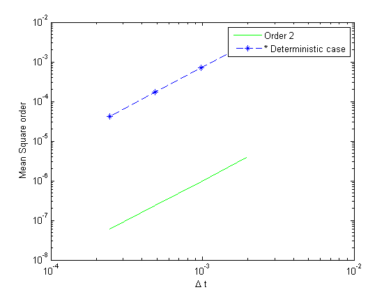 Figure 1
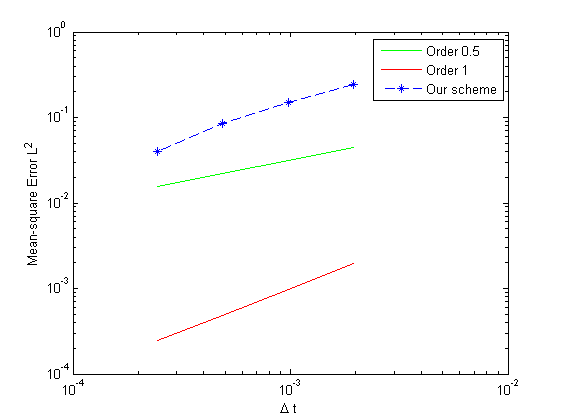 Figure 2
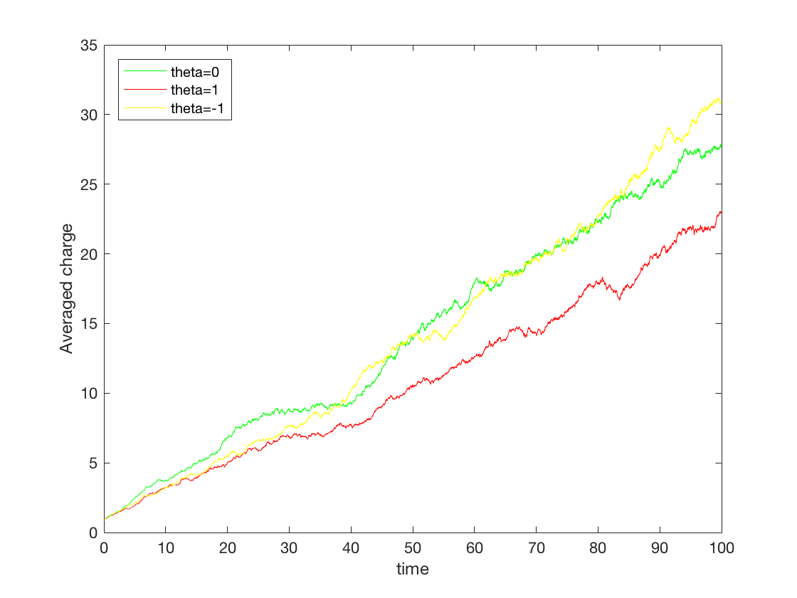 Figure 3
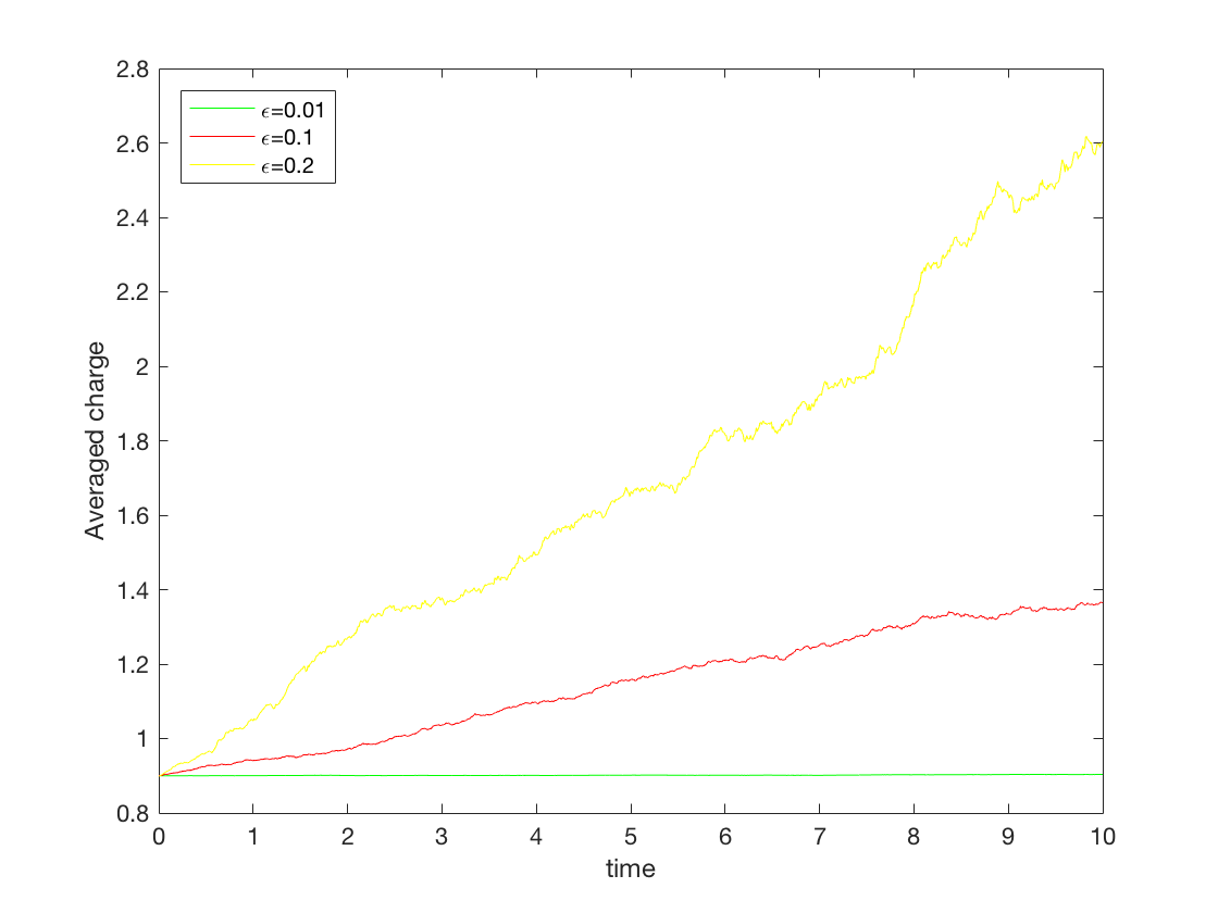 Figure 4
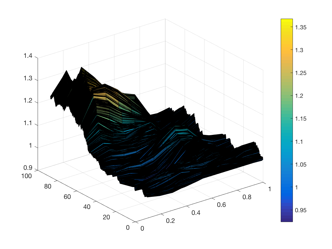 Figure 5
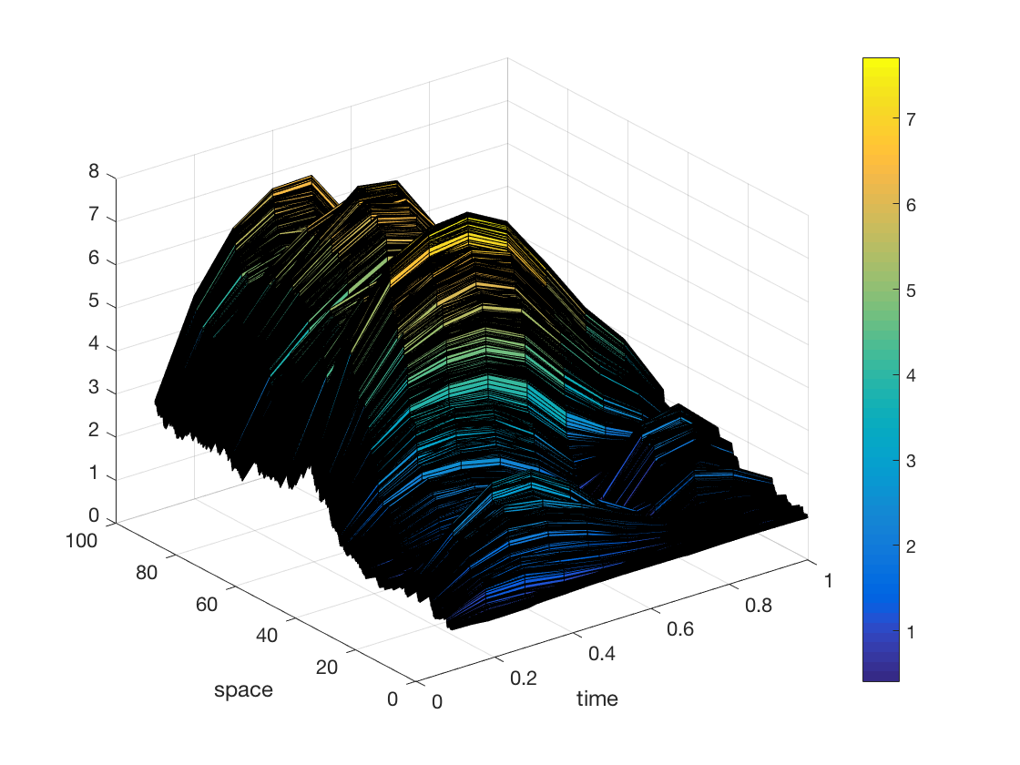 Figure 6
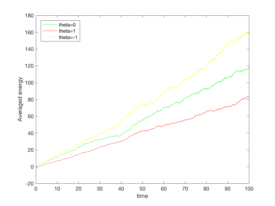 Figure 7
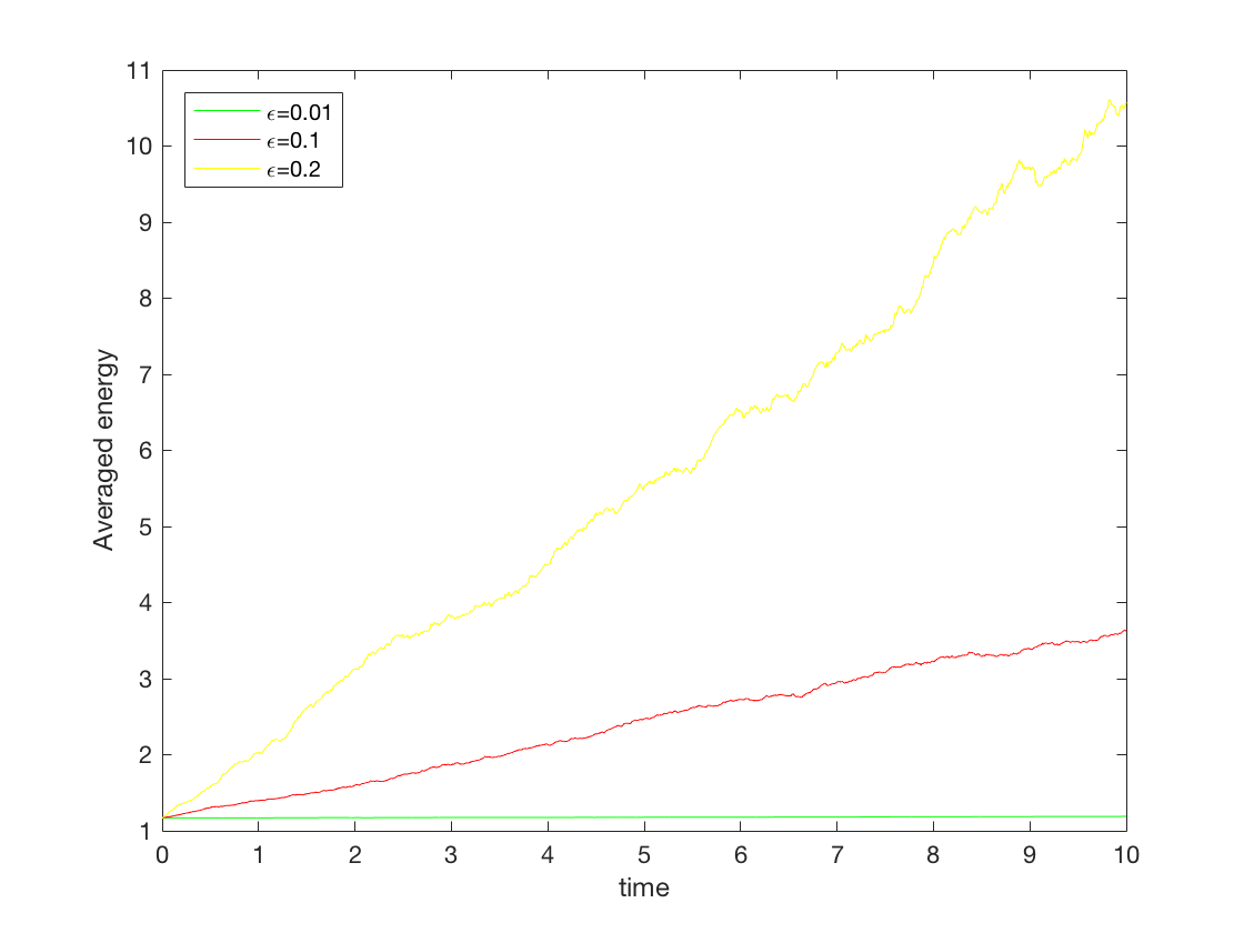 Figure 8
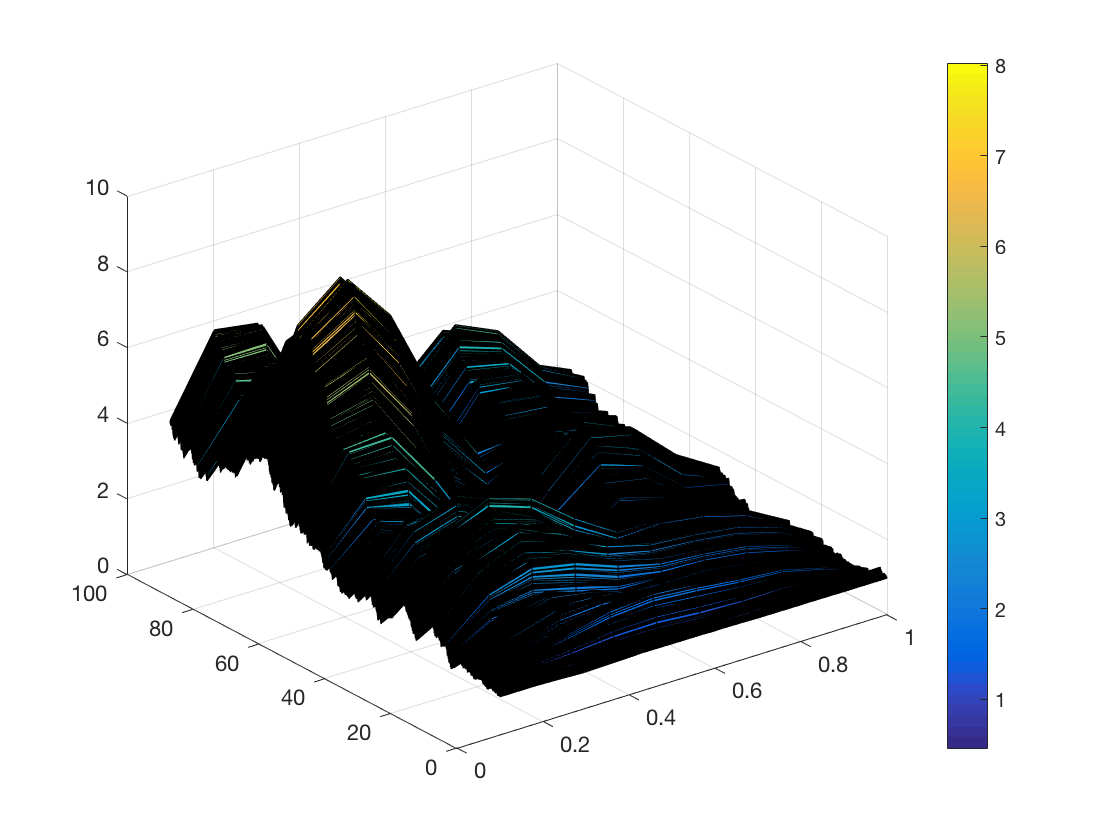 Figure 9
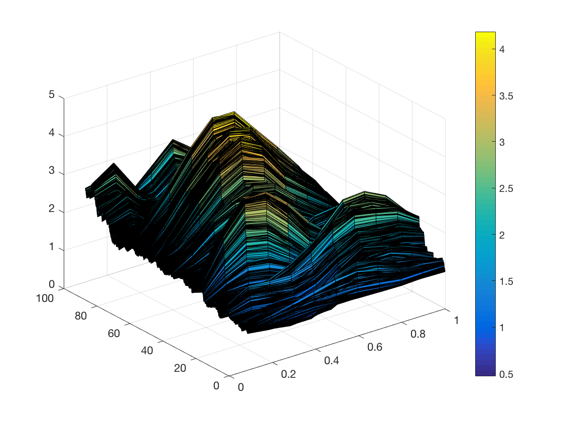 Figure 10
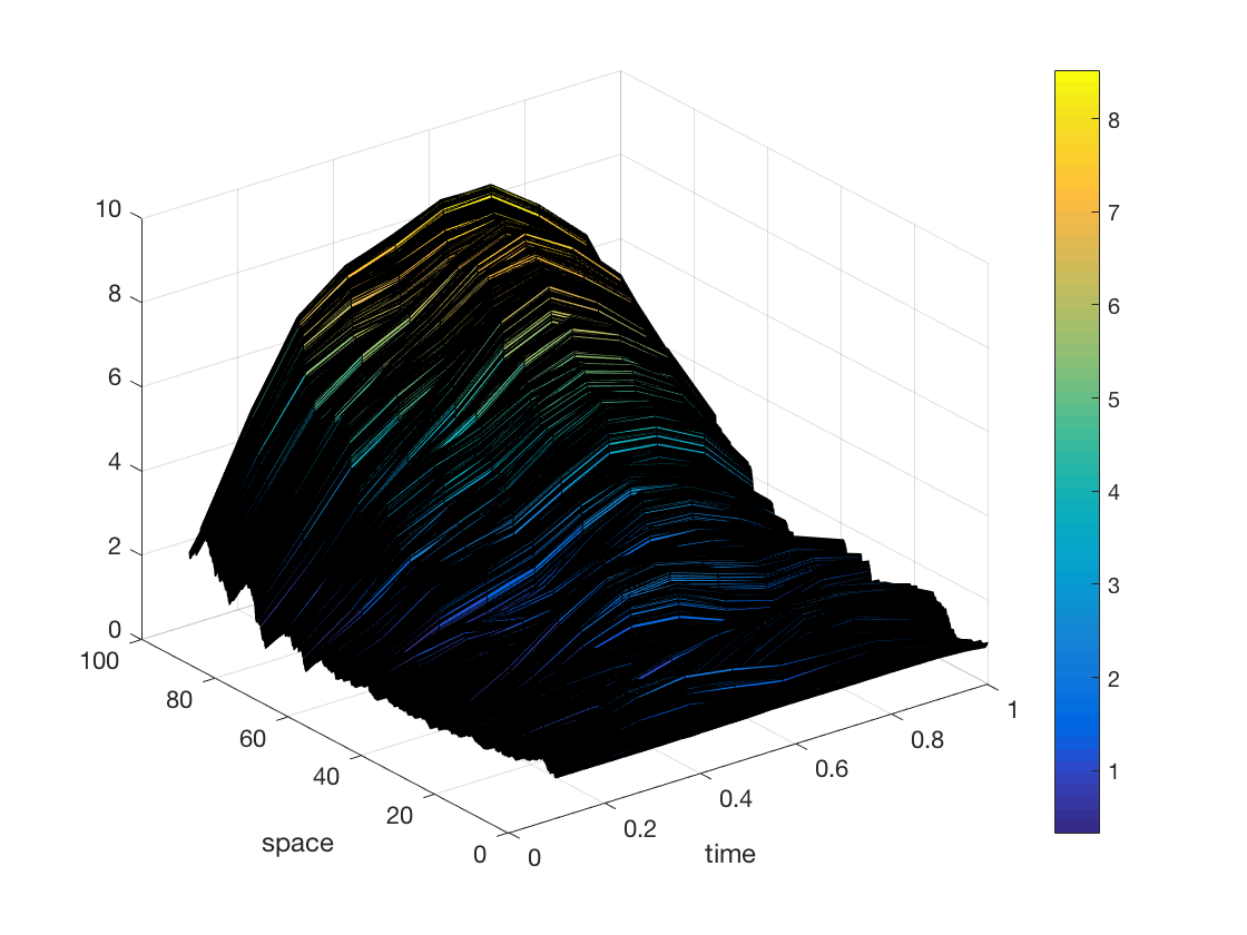 Figure 11
Peer Reviews
No public reviews on file for this paper yet. If you reviewed it on a platform where reviews are public (OpenReview, ICLR, NeurIPS, ICML), you can paste yours below so the community can read it here.
Videos
No videos yet. Explain this paper in a talk, walkthrough, or lecture? Add one.
Taxonomy
TopicsAdvanced Mathematical Physics Problems · Stochastic processes and financial applications · Financial Markets and Investment Strategies
Convergence analysis of a symplectic semi-discretization for stochastic NLS equation with quadratic potential
Jialin Hong
Institute of Computational Mathematics and Scientific/Engeering Computing, AMSS, Chinese Academy of Sciences, Beijing, 100190, P.R. China
School of Mathematical Science, University of Chinese Academy of Sciences, Beijing, 100049, China
,
Lijun Miao
School of Mathematics, Liaoning Normal University, Dalian, 116029, P.R. China
[email protected] (corresponding author )
and
Liying Zhang
Department of Mathematics, College of Sciences, China University of Mining and Technology, Beijing 100083, China.
Abstract.
In this paper, we investigate the convergence in probability of a stochastic symplectic scheme for stochastic nonlinear Schrödinger equation with quadratic potential and an additive noise. Theoretical analysis shows that our symplectic semi-discretization is of order one in probability under appropriate regularity conditions for the initial value and noise. Numerical experiments are given to simulate the long time behavior of the discrete average charge and energy as well as the influence of the external potential and noise, and to test the convergence order.
Key words and phrases:
stochastic nonlinear Schrödinger equation, quadratic potential, additive noise, stochastic symplectic scheme, stochastic multi-symplectic scheme
2010 Mathematics Subject Classification:
60H15, 60H35, 65P10
1. Introduction
In this paper, we consider the following stochastic nonlinear Schrödinger equation with quadratic potential and additive noise
[TABLE]
where , , , , and denotes a Wiener process expressing the random perturbations ([14]). This equation models Bose–Einstein condensations under a magnetic trap when , where the quadratic potential describes the magnetic filed whose role is to confine the movements of particles ([4]). [11] and [15] establish the well-posedness and blow up of the solution for (1.1). The authors in [15] indicate that the additive noise rather than the potential dominates the dynamical behaviors of the solutions.
It is known that numerical approximations have become an important tool to investigate the behaviors of the solutions. In order to guarantee the reliability and effectiveness of numerical solutions for longtime simulations, we expect numerical methods to preserve the intrinsic properties of the original systems as much as possible. For Hamiltonian systems, the symplectic schemes are shown to be superior to conventional ones especially in long time computation, artributed to their preservation of the qualitative property and the symplectic structure of the underlying continuous systems. The main goal of this work is to analyze the convergence rate of the symplectic scheme for (1.1). We propose a mid-point method in temporal direction of (1.1) in order to preserve the properties of the original problems as much as possible and to effectively simulate the influence of the external potential and noise on the long time behavior of the solution. It is shown that the mid-point semi-discretization is a symplectic scheme which preserves the symplectic structure of (1.1). The interested readers are referred to [2] and references therein for the numerical simulation of the deterministic Schrödinger equation with potentials. We also refer to [5] for the convergence analysis of the mid-point method applied to the stochastic Schrödinger equation with Lipschitz coefficients, to [6] for the mean-square convergence of a symplectic local discontinuous Galerkin method to stochastic linear Schrödinger equation with a potential and multiplicative noise and to [1] for the strong convergence rate of stochastic exponential method to the stochastic linear Schrödinger equations with a multiplicative potential.
Furthermore, we give the convergence order of the proposed scheme under non-Lipschitz condition. To this end, the higher regularity of the solution is needed due to the effect of semigroup. We get the stability of solution of (1.1) in by means of the estimates for the high moments of charge and energy. Because the nonlinear term of (1.1) is not global Lipschitz, it is difficult to analyze the convergence order of the symplectic scheme. Here we use the truncated technique to get the truncated equation whose nonlinear term is global Lipschitz. Then we prove that the convergence order is one in probability for the symplectic scheme under appropriate hypothesis on initial value and noise. In addition, we simulate the long time behavior of the discrete average charge and energy under the influence of the external potential and noise using a stochastic multi-symplectic scheme, owing to the multi-symplecticity of (1.1). Here we cite [12] and [13] as a partial list of the publications on the multi-symplectic scheme for the deterministic and stochastic Schrödinger equations. Numerical experiments present that the noise dominates the dynamics of the solution stronger than external potential.
The rest of the paper is organized as follows. Some properties of the solution, including the evolution law of charge, the uniform boundedness of energy and solution, are given in Section 2. In Section 3, we first show that (1.1) owns the stochastic symplectic structure, then we construct a stochastic symplectic scheme and prove that its temporal order of convergence is one in probability. In Section 4, we perform numerical experiments to test the convergence order in Section 3, and to simulate the long time behavior of the discrete average charge and energy under the influence of the external potential and noise. In the remainder of the article, is a generic constant whose value may vary in different occurrences, denotes the constant depending on some parameters.
2. Stochastic NLS equation with quadratic potential
In order to state precisely Eq. (1.1), we consider the probability space endowed with a normal filtration . Let with and being its real and imaginary parts, respectively. We assume that is a family of real-valued independent indentified Brownian motions. Let be an orthonormal basis of some Hilbert space . We consider the complex valued Wiener process
[TABLE]
where the space of Hilbert–Schmidt operators from to another Hilbert space . The corresponding norm is then given by
[TABLE]
In addition, denotes Hilbert space with inner product for . is denoted by , where is Sobolev space consisting of functions such that exist and are square integrable for all is positive integer. Throughout the paper, we assume that for a certain parameter , and Sobolev space will be used .
Now, we recall the mild solution of Eq. (1.1) from [8].
An -valued -adapted process is called a mild solution of (1.1) if for every holds -a.s.
[TABLE]
where denotes the semigroup of solution operator of the deterministic linear differential equation
[TABLE]
If the noise term is eliminated in (1.1), then it is the deterministic nonlinear Schrödinger equation with the quadratic potential
[TABLE]
it possesses the charge conservation law
[TABLE]
and energy conservation law
[TABLE]
But these conservation laws of Eq. (1.1) are invalid. Now, we state its charge evolution law and energy evolution laws, respectively.
Lemma 2.1**.**
Eq. (1.1) has the following global charge evolution law a.s.
[TABLE]
Moreover, for any there exists a constant
[TABLE]
Proof.
The proof is based on the application of Itô formula to functional Since is Fréchet derivable, the derivatives of along directions and are as follows:
[TABLE]
From Itô formula, we have
[TABLE]
To prove (2.5), we apply Itô formula to
[TABLE]
Taking the supremum and using a martingale inequality yields
[TABLE]
The lemma is proved using Hölder and Young’s inequalities in the second term of the right hand side and an induction argument. ∎
Taking expectation in both sides of (2.4), we have that
[TABLE]
The formula (2.6) indicates that the average charge is linear growth with respect to time Next, we present the energy evolution law of (1.1), which can be proved by Itô formula too.
Lemma 2.2**.**
Eq. (1.1) has the following global energy evolution law a.s.
[TABLE]
From the definition of energy in (2.3) and Gagliardo–Nirenberg’s inequality, we can conclude the following result.
Lemma 2.3**.**
*Assume that . There exist constants and such that
(i) if , then
(ii) if , then *
Using this lemma, we get the uniform boundedness of .
Lemma 2.4**.**
Let , , . There exists a constant such that
[TABLE]
Proof.
We first consider the case of . If applying the expectation to (2.2), we have
[TABLE]
the assertion (i) holds. If
[TABLE]
Since Hölder inequality, Young’s inequality and Gagliardo–Nirenberg’s inequality, we have
[TABLE]
the last inequality follows from Lemma 2.3 and is embedded into . Therefore,
[TABLE]
Then we use Gronwall’s inequality to get the assertion (i).
If we apply Itô formula to \big{(}H(u)\big{)}^{p}, then
[TABLE]
Since the second term on the right-hand side vanishes after taking expectation, there remains to estimate the third term and the last term. For the third term, there exists a constant such that
[TABLE]
The operator is bounded from into . Furthermore, is embedded into , is also bounded from into and Young’s inequality, so we obtain
[TABLE]
From Gagliardo–Nirenberg’s inequality and
[TABLE]
Substituting (2.11) into (2), and combining with (2.5) and Lemma 2.3, we have
[TABLE]
For the last term in (2), due to Young’s inequality, Lemma 2.3 and is embedded into we get
[TABLE]
Because of (2), (2), and Hölder inequality, we deduce
[TABLE]
we apply Gronwall’s inequality to obtain the estimate (i).
To show the assertion (ii) for we take the supremum over in (3) before taking the expectation. The main difference is the appearance of the supremum of a stochastic integral compared to assertion (i). This term can be estimated by a martingale inequality,
[TABLE]
The assertion (ii) for uses arguments similar to the above estimate, so we skip the details here. ∎
In [8], Theorem 4.6, a uniform boundedness for the energy is used to construct a unique mild solution with continuous -valued paths for stochastic nonlinear Schrödinger equation. We can follow the same strategy to construct the unique global mild solution with continuous -valued paths using Lemma 2.4.Moreover, we can get the same result in and have the following uniform boundedness of the solution under . Similar to Theorem 2.1 of [7], The proof of the stability of solution in Sobolev space is directly obtained by analyzing the functional
[TABLE]
Lemma 2.5**.**
Let , , and . There exists a constant such that
[TABLE]
3. Stochastic symplectic scheme
As we all know, the stochastic Schrödinger equation without quadratic potential is an infinite-dimensional stochastic Hamiltonian system, which characterize the geometric invariants of the phase flow and contribute to constructing the numerical schemes for long time computation. In the following, we show that Eq. (1.1) possesses stochastic symplectic structure.
Denote by and the real and imaginary parts of , respectively. Let be a cylindrical Wiener process with and being its real and imaginary parts. Then the Wiener process . Then Eq. (1.1) is equivalent to
[TABLE]
with initial datum Set
[TABLE]
Then the equation (3) can be rewritten as
[TABLE]
where and denote the variational derivative of with respect to and , respectively. In fact, (3) is an infinite-dimensional stochastic Hamiltonian system. Using the same procedure as [5], one can derive that (3) possesses the symplectic structure
[TABLE]
Theorem 3.1**.**
The phase flow of Eq. (1.1) preserves the symplectic structure (3.3).
In order to preserve the stochastic symplectic structure, we consider the mid-point scheme of the temporal discretization for (1.1),
[TABLE]
where is time step size, , Denote
[TABLE]
we have the following result.
Theorem 3.2**.**
The scheme (3.4) possesses the discrete symplectic structure, i.e.
[TABLE]
Proof.
For convenience, denote then (3.4) can be rewritten as
[TABLE]
Differentiating the above equation on the phase space, we obtain
[TABLE]
Then
[TABLE]
Substituting
[TABLE]
into the above equality, we have
[TABLE]
∎
In fact, we can prove that the scheme (3.4) exists a numerical solution.
Proposition 3.1*.*
Let and be -measurable with values in , then for sufficiently small , there exists an -valued -adapted solution of (3.4) .
Proof.
Fix a family of deterministic functions in , we also fix the existence of solution of
[TABLE]
follows from a standard Galerkin method and Brouwer theorem (see [9]). Assuming that is a solution of (3.5), multiplying (3.5) by the complex conjugate of , integrating over and taking the imaginary part of the resulting identity, we have
[TABLE]
Therefore,
[TABLE]
Using the same method, we multiply (3.5) by integrate over and take the imaginary part of the resulting identity. Therefore, using Hölder inequality and Young’s inequality, we obtain
[TABLE]
where the second inequality follows from Gagliardo–Nirenberg’s inequality and the last inequality follows from the fact that is sufficiently small. From (3.6) and Lemma 2.3, we have
[TABLE]
Define a map
[TABLE]
where is the set of subsets of , is the set of solutions of (3.5). From the closedness of the graph of and a selector theorem, there exists a universal and Borel measurable map such that for Assume that is -measurable random variable, then is -valued solution of (3.4). ∎
Now we investigate the convergence rate of the scheme (3.4) under . To deal with the power law of the nonlinear term, we introduce a cut-off function such that and on (see [10]). Write \mu_{R}(u)=\mu\big{(}\frac{\|u\|_{H^{1}}}{R}\big{)}, then we consider the truncated equation
[TABLE]
Denote f(u_{R})=\mu_{R}(u_{R})\big{(}|u_{R}|^{2}u_{R}\big{)}, the mild form of the corresponding mid-point scheme of (3.7) is
[TABLE]
where
[TABLE]
We have the following estimates to operators and ( [10]) with , which are are useful in the convergence analysis below :
[TABLE]
[TABLE]
The scheme (3.8) is well-defined and are uniformly bounded provided that the nonlinear term is global Lipschitz. This Lipschitz continuity can be guaranteed by Proposition 2.2 in [3] because is an algebra.
Assume that , . From the global Lipschitz continuity of the nonlinear term, we obtain that
[TABLE]
and
[TABLE]
using Sobolev embedding and Gronwall’s inequality. Now, we prove the following error estimate, the key of its proof lies in the mild solution and the unitarity of the both and .
Proposition 3.2*.*
Let , and , then for any , there exists a constant such that
[TABLE]
Proof.
For simplicity, we omit the dependence of and . Assume that , here denotes the Lipschitz constant of . Clearly,
[TABLE]
Define the mapping which maps to . For any sequences and with we have
[TABLE]
This fact provides that
[TABLE]
We know that
[TABLE]
and deduce
[TABLE]
From (3.9), the terms and are estimated as following,
[TABLE]
For the term , we divide it into the following parts
[TABLE]
Concerning the first term , we have
[TABLE]
so that
[TABLE]
In the context of mild solution of (3.7), we have
[TABLE]
Therefore,
[TABLE]
For is an isomery and
[TABLE]
Thus,
[TABLE]
which leads to
[TABLE]
Because , we have
[TABLE]
Due to , we get
[TABLE]
Using Fubini’s theorem and martingale inequality, we have
[TABLE]
For ,
[TABLE]
Using the definition of , we can estimate similarly.
It remains to estimate the term It can be decomposed into a sum
[TABLE]
For the term , we have
[TABLE]
Similar to the estimates of , we have
[TABLE]
Therefore,
[TABLE]
Using the definition of the mild solution and Taylor formula,
[TABLE]
Combined with the estimate of and (3.10),
[TABLE]
For the term , the estimate of and Lipschitz continuity of yield that
[TABLE]
Summarize the above estimates, we obtain
[TABLE]
Then, by (3.11) and Minkowski inequality, we have
[TABLE]
The result follows from the discrete Gronwall’s inequality. ∎
Theorem 3.3**.**
Let , and , then for any ,
[TABLE]
Proof.
Define a stopping time
[TABLE]
and the discrete solution if From Proposition 3.2, for any ,
[TABLE]
This yields that converges to 0 in probability as . Similar to [10], by Chebyshev inequality, we have
[TABLE]
Following from the uniform boundedness of and together with Proposition 3.2, we have \mathbf{P}\big{(}\max_{n=0,\cdots,N}\|u(t_{n})-u^{n}\|_{H^{1}}\geq C\tau\big{)} converges to 0 as and tend to ∎
4. Numerical experiments
In this section, we focus on the following example
[TABLE]
Here, denotes the size of noise and can be considered as the deterministic case in some sense. Next, we first present numerical experiments to verify the convergence order of the proposed stochastic symplectic scheme (3.4) on . In order to investigate the influence of quadratic potential and noise, we give some numerical experiment on the solution and evolution laws of charge and energy in the sense of expectation for stochastic multi-symplectic scheme
[TABLE]
where
[TABLE]
It is obtained by applying mid-point scheme to (4.1) in both temporal and spatial directions [13].
Under the homogeneous Dirichlet boundary condition, (4) possesses the discrete charge and energy properties deduced by similar method to [13], respectively:
[TABLE]
and
[TABLE]
Here, the global energy of (4) at time is defined as
[TABLE]
In the sequel, we choose , and consider the real-valued Wiener process with the truncated number , where is a family of independent –valued Brownian motions, and denotes the orthonormal basis of . Let be the uniform discretization of of size , and apply the uniform discretization of of size . The reference values are generated for the smallest mesh size In Fig.4.1, we plot the convergence curves based on the errors with We can see that the convergence order for the -error of the mid-point scheme is 2 if and the slope of our scheme (3.4) in stochastic case is 1. This observation verifies the theoretical result in Section 3.
We now investigate the behaviors of solitary wave solution under the influence of quadratic potential and noise. In these experiments, we take and the step sizes , . The profiles of amplitude are presented in Fig.4.2 and Fig.4.3. In Fig.4.2, these two figures give the propagation of solitary wave when taking different size of noise and . We find that the waveform of solution is obviously disturbed as the scale of noise becomes larger, that is the velocity of solitary wave is influenced. Fig.4.3 presents the long time behaviors of solution when we take the different kind of quadratic potential with . Combining these three figures, we find that the external potential influences the velocity of solitary wave, it can neither prevent the propagation, nor destroy the solitary. Moreover, it dominates the dynamics of the solution weaker than noise.
The average charge conservation law follows linearly grow evolution law with respect to time and the average energy conservation law follows linear evolution law at most. These phenomena are reflected in Fig.4.4 and Fig4.5, respectively, where the evolution of the average discrete charge and energy obey nearly linear growth over 100 trajectories. In Fig.4.4, the different external potential have small effects on the average charge and energy. But different size noises have obvious effects on them, the evolution laws of the charge and energy more and more tend to the conservation laws when tends to [math] especially.
The reference list from the paper itself. Each links out to its DOI / PubMed record.
- 1[1] R. Anton and D. Cohen. Exponential integrators for stochastic Schrödinger equations driven by itô noise. To appear in the special issue on SPD Es of J. Comput. Math.
- 2[2] W. Bao and Y. Cai. Mathematical theory and numerical methods for Bose-Einstein condensation. Kinet. Relat. Models , 6(1):1–135, 2013.
- 3[3] R. Belaouar, A. de Bouard, and A. Debussche. Numerical analysis of the nonlinear Schrödinger equation with white noise dispersion. Stoch. Partial Differ. Equ. Anal. Comput. , 3(1):103–132, 2015.
- 4[4] R. Carles. Critical nonlinear Schrödinger equations with and without harmonic potential. Math. Models Methods Appl. Sci. , 12(10):1513–1523, 2002.
- 5[5] C. Chen and J. Hong. Symplectic Runge–Kutta semidiscretization for stochastic Schrödinger equation. SIAM J. Numer. Anal. , 54(4):2569–2593, 2016.
- 6[6] C. Chen, J. Hong, and L. Ji. Mean-square convergence of a symplectic local discontinuous Galerkin method applied to stochastic linear Schrödinger equation. IMA J. Numer. Anal. , 37(2):1041–1065, 2017.
- 7[7] J. Cui, J. Hong, and Z. Liu. Strong convergence rate of finite difference approximations for stochastic cubic Schrödinger equations. J. Differ. Equ. , 263(7):3687–3713, 2017.
- 8[8] A. de Bouard and A. Debussche. The stochastic nonlinear Schrödinger equation in H 1 superscript 𝐻 1 H^{1} . Stochastic Anal. Appl. , 21(1):97–126, 2003.