Relation between Regge calculus and BF theory on manifolds with defects
Marcin Kisielowski

TL;DR
This paper establishes a connection between Regge calculus and BF theory by constructing manifolds with defects from simplicial complexes, enabling a reformulation of Regge geometry in terms of topological BF theory.
Contribution
It introduces a method to encode Regge geometry within BF theory on manifolds with defects, bridging discrete geometry and topological field theory.
Findings
The constructed action matches the standard BF action for regular manifolds.
Solutions of the field equations reproduce Regge actions at boundary data.
Degrees of freedom are transferred from Regge calculus to BF theory.
Abstract
In Regge calculus the space-time manifold is approximated by certain abstract simplicial complex, called a pseudo-manifold, and the metric is approximated by an assignment of a length to each 1-simplex. In this paper for each pseudomanifold we construct a smooth manifold which we call a manifold with defects. This manifold emerges from the purely combinatorial simplicial complex as a result of gluing geometric realizations of its n-simplices followed by removing the simplices of dimension n-2. The Regge geometry is encoded in a boundary data of a BF-theory on this manifold. We construct an action functional which coincides with the standard BF action for suitably regular manifolds with defects and fields. On the other hand, the action evaluated at solutions of the field equations satisfying certain boundary conditions coincides with an evaluation of the Regge action at Regge geometries…
Click any figure to enlarge with its caption.
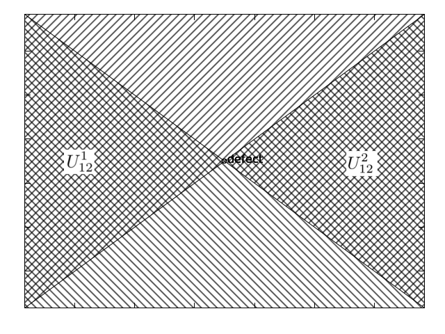 Figure 1
 Figure 2
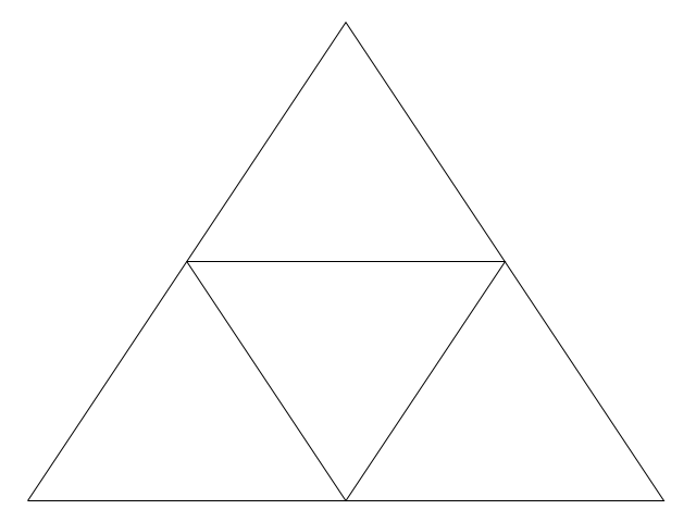 Figure 3
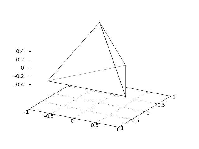 Figure 4
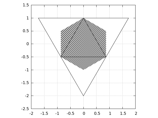 Figure 5
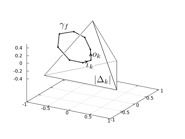 Figure 6
 Figure 7
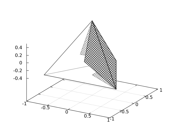 Figure 8
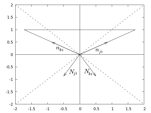 Figure 9
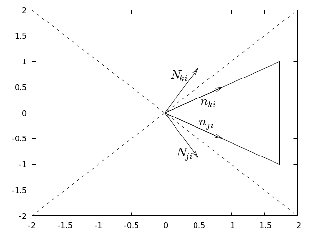 Figure 10
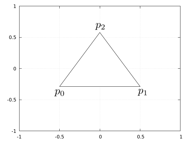 Figure 11
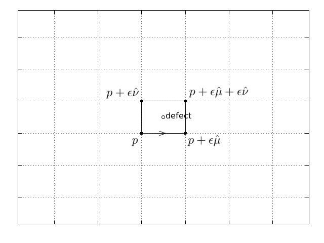 Figure 12
 Figure 13
Peer Reviews
No public reviews on file for this paper yet. If you reviewed it on a platform where reviews are public (OpenReview, ICLR, NeurIPS, ICML), you can paste yours below so the community can read it here.
Videos
No videos yet. Explain this paper in a talk, walkthrough, or lecture? Add one.
\typearea
[10mm]12
Relation between Regge calculus and BF theory on manifolds with defects
Marcin [email protected]
1* Institute for Quantum Gravity, Chair for Theoretical Physics III,
University of Erlangen-Nürnberg, Staudtstraße 7 / B2, 91058 Erlangen, Germany
2 Instytut Fizyki Teoretycznej, Uniwersytet Warszawski,
ul. Pasteura 5, 02-093 Warsaw, Poland*
Abstract
In Regge calculus the space-time manifold is approximated by certain abstract simplicial complex, called a pseudo-manifold, and the metric is approximated by an assignment of a length to each 1-simplex. In this paper for each pseudomanifold we construct a smooth manifold which we call a manifold with defects. This manifold emerges from the purely combinatorial simplicial complex as a result of gluing geometric realizations of its n-simplices followed by removing the simplices of dimension n-2. The Regge geometry is encoded in a boundary data of a BF-theory on this manifold. We construct an action functional which coincides with the standard BF action for suitably regular manifolds with defects and fields. On the other hand, the action evaluated at solutions of the field equations satisfying certain boundary conditions coincides with an evaluation of the Regge action at Regge geometries defined by the boundary data. As a result we trade the degrees of freedom of Regge calculus for discrete degrees of freedom of topological BF theory.
1 Introduction
1.1 Motivation
Our motivation for this research comes from the spin-foam approach to Quantum Gravity [1, 2, 3, 4, 5, 6, 7, 8, 9, 10]. The spin-foam models can be thought to be quantum versions of Regge calculus. They are based on the observation made by Ponzano and Regge [11] that an algebraic object called -symbol, appearing in recoupling theory of 4 quantum angular momenta, relates to the Regge action for 3-dimensional Euclidean gravity. This result has been extended to the physical case: 4-dimensional Lorentzian gravity. Such generalized symbol is called a vertex amplitude and is a basic building block of the so-called EPRL/FK spin-foam model [12, 13, 14, 15, 16, 17, 18, 19, 20, 21, 22, 23]. The derivation of the spin-foam model is based on the Plebański formulation of Gravity as a theory of BF type [24]. The spin-foam model is obtained by triangulating the space-time manifold, constructing a discrete path integral for BF theory and imposing the constraint on the 2-simplices of this triangulation.
If we remove the 2-simplices of the triangulation, we obtain a manifold with defects. As claimed in [25] spin-foam models can be interpreted as topological theories of BF type on such manifolds with defects. In fact, the vertex amplitude for the Lorentzian model with non-zero cosmological constant has been recently introduced as the Chern-Simons expectation value of certain Wilson-graph operator [26, 27, 28, 29].
In this paper we study a classical relation between the (topological) BF theory [30, 31, 32, 33, 34, 35] and Regge calculus [36]. Let us consider a triangulation of space-time. The Einstein-Hilbert action evaluated at locally flat metrics singular at the 2-simplices of the triangulation coincides with the Regge action [37] (see also [38]). In fact we can remove the 2-simplicies (together with appropriate neighborhood), creating thus a manifold with defects, and evaluate the Einstein-Hilbert action with the Gibbons-Hawking-York boundary term [39, 40] at appropriate locally flat metric. When evaluated on such metrics the interior part of the action vanishes and the boundary term becomes the Regge action [25]. This provides some classical justification for the interpretation of spin-foam models as topological theories of BF type on manifolds with defects. It is however not fully satisfactory. The first reason is that Einstein‘s theory of General Relativity is not a topological theory. When viewed as a theory of BF-type it involves constraints that are imposed not only at the boundary but also in the interior. If we relax these conditions and impose the constraints only at the boundary, we obtain a topological field theory (BF theory). In fact, we will show that the BF action evaluated at solutions of its field equations satisfying certain boundary conditions coincides with an evaluation of the Regge action at Regge geometries defined by the boundary data. Therefore we trade the topological degrees of freedom of the BF theory for the discrete degrees of freedom of Regge calculus. Second reason is that the locally flat metric is not the only solution of the Einstein‘s equations but this is the case for the BF theory. The third reason is that in the previous approach a starting point was a smooth space-time which is triangulated afterwards, whereas spin foams (and related to them Group Field Theories) refer to a combinatorial structure of abstract complexes and the space-time emerges as build from some basic building blocks [41, 42, 43, 44, 45, 46]. Such combinatorial characterization gives a better control over possible histories of quantum gravitational field. In this paper we will start with an abstract simplicial complex equipped with certain geometric structure and from this data we will construct a smooth manifold with defects. This approach will be more general than the previous approach because each manifold with defects obtained by removing simplicial complexes from the triangulation can be obtained by our procedure but we will obtain also manifolds with defects that cannot be completed to manifolds without defects.
1.2 Motivating example and our hypothesis
The basic building block of the Regge geometries is the -cone metric [36]. The simplest example of such metric is the metric on a 2-dimensional cone with the apex removed, i.e. on , induced by the flat metric on :
[TABLE]
where is the apex angle of the cone. A generalization of this metric to three dimensions is the -cone metric on :
[TABLE]
Let us switch to the triad formalism:
[TABLE]
where is a basis of the su(2) Lie algebra defined by the Pauli matrices . We denote by an invariant (positive-definite) scalar product on su(2) in which the basis is orthonormal. The -cone metric is related to the internal metric by the standard relation:
[TABLE]
for any . The connection 1-form is:
[TABLE]
Although the connection is flat
[TABLE]
on a holonomy around any loop encircling the defect is non-trivial
[TABLE]
It is the rotation by an angle preserving the direction of the defect. The angle is called a deficit angle.
The fact that a holonomy of a flat connection on a non-simply connected manifold can be non-trivial is a basis of mathematical formulation of the Aharonov-Bohm effect [47]. The defect models long and infinitely thin solenoid. Outside the solenoid the magnetic field (i.e. curvature form) vanishes but the magnetic flux through a surface cutting the solenoid transversely into two pieces is non-trivial. This can be interpreted as the fact that the magnetic field (i.e. curvature form) is concentrated on the defect:
[TABLE]
Indeed, with this interpretation of the curvature, we recover the (abelian) Stokes‘ theorem:
[TABLE]
where is any surface which boundary is .
In three dimensions the triad coincides with the -field and Palatini action coincides with the BF action:
[TABLE]
Let us note that outside of the defect, i.e. on , the configuration presented above satisfies the field equations:
[TABLE]
Although is only defined on the manifold with defect (), we can use the extended definition of the curvature form (1) to extend the measure
[TABLE]
to the manifold without defect (). Remarkably, the evaluation at such configuration
[TABLE]
coincides with (a part of) the Regge action if we interpret the number as a length of an edge (the defect) and the angle as a deficit angle associated to this edge. We expect that it is a general feature: * BF action evaluated at solutions of its field equations satisfying certain boundary conditions coincides with an evaluation of the Regge action at Regge geometries defined by the boundary data.*
1.3 Illustration of the construction of the action functional
The example above is very simple and is missing some essential features of the construction presented in this paper. One of the simplifications is that the flat connection is reducible: the holonomy matrix is an element of the abelian subgroup of the structure group . Thanks to this abelian Stokes‘ theorem can be used. Another simplification is that the manifold with defect can be completed to a manifold without defect. We will use a more general definition of manifold with defects where this will not always be possible. A way out to deal with both problems is to define the action functional as a Riemann-like series. This solves the first problem because the surface ordered integral from the non-abelian version of the Stokes‘ theorem [48] can be approximated by a regular surface integral for small loops. This infinitesimal version of the Stokes theorem has in fact been used in [48] to derive the non-abelian Stokes theorem. We will solve the second problem by appropriately choosing the lattice: such that only the data on the manifold with defects will be used. Let us illustrate this idea on the following example. Let us consider a connection and a triad on . We do not assume that the connection is flat or trosionless. We introduce the following cubical lattice:
[TABLE]
where is the lattice constant. We assume that for some positive natural number . For each point we consider a holonomy along a plaquette (see for example [49]) containing the points:
[TABLE]
where , . Let be an element of the so(3) Lie algebra such that
[TABLE]
We define the following functional
[TABLE]
Clearly, it is gauge invariant. If the fields and are defined by a restriction to of global 1-forms on (in particular, if the SO() principal fibre bundle over is trivial), then in the limit of lattice constant going to [math] we recover the BF action:
[TABLE]
Let us consider a flat connection (not necessarily torsionless) and a triad on . We introduce a covering of with two open sets:
[TABLE]
The intersection is formed by two disjoint components (see figure 1(b)):
[TABLE]
Clearly is gauge invariant. Let us fix the gauge such that the local connection 1-forms and defined on and , respectively, vanish:
[TABLE]
In this gauge the transition function is locally constant (see for example [50]):
[TABLE]
A triad defines and is defined by local 1-forms and defined on and , respectively. The so(3)-valued matrices defined by holonomies by relation (3) have the following properties:
[TABLE]
where is given by:
[TABLE]
Due to these properties the only non-zero contributions to come from points in the set . The limit becomes
[TABLE]
where is the integral of over the defect
[TABLE]
The action functional is similar to a part of the action functional in the tetrad formulation of the Regge calculus [51, 52]. The role of discretized triad is played by the vector and the role of discretized connection is played by (locally constant) transfer matrices of a flat bundle.
2 The space-time as a simplicial complex
In this section we describe the space-time as certain simplicial complex equipped with a geometric structure.
An abstract simplicial complex is a collection of non-empty finite sets called abstract simplices such that every non-empty subset of an abstract simplex in is an abstract simplex in [53, 54]. Every non-empty subset of an abstract simplex is called a face of . We will write if is face of . In the following we will restrict to finite complexes, i.e. to complexes that are finite sets. Any element of an abstract simplex is called a vertex of . A simplex with vertices is said to have dimension and will be called an -simplex. The maximum of the dimensions of simplices contained in is called the dimension of the complex and will be denoted by . We will denote by the set of all -simplices in . Clearly .
A pseudo-manifold [55] of dimension is a finite -dimensional simplicial complex with the following properties:
- •
each (n-1)-dimensional simplex is a face of precisely two -dimensional simplices,
- •
any two -simplices and can be connected by a chain of simplices such that is an -dimensional simplex,
- •
each simplex is a face of some -simplex.
We will further assume that the pseudomanifold is orientable, i.e. [56]. We will denote by a representative of the generator of this homology group.
We will now introduce additional structure on a pseudo-manifold, which we will call a geometric structure. This structure is equivalent to assigning lengths to edges in the Regge calculus and will carry the information about the orientation. Let us first recall the definition of a (geometric) -simplex [53]. A set of points in is called (affinely) independent if the system of vectors
[TABLE]
is linearly independent. A convex hull of a set of independent points in is called a (geometric) -simplex in . Let us denote by the -dimensional simplices of . Consider a family of maps , assigning a set of independent points in to the set of vertices of a simplex . Each map will be called a geometric realization of the (abstract) simplex . We will use the following notation:
[TABLE]
where denotes the convex hall of a set of points. We will call geometric simplices. By we will denote a barycenter of a (geometric) simplex:
[TABLE]
We will assume that each geometric simplex has an orientation that agrees with the standard orientation of , i.e.
[TABLE]
where is the Levi-Civita symbol such that . We say that two maps and are compatible if one of the following conditions is satisfied:
- •
,
- •
there is an affine isometry of the Euclidean/Minkowski space preserving the orientation such that
[TABLE]
Remark 1**.**
Maps are unique. The condition (5) specifies an affine isometry uniquely up to reflection about the hyperplane defined by points . Let be the unique element in and be the unique element in . The points and are on opposite sides of because the complex is orientable, the orientation of each geometric simplex has an orientation that agrees with the standard orientation of and is orientation preserving. This fixes the remaining ambiguity.
A geometric structure on an -dimensional pseudo-manifold is a family of pairwise compatible maps . The maps have the following properties:
[TABLE]
We will call it a gluing pattern. We say that two geometric structures and are equivalent if there exist affine isometries such that
[TABLE]
Example 1**.**
Let be a -dimensional pseudomanifold with Euclidean geometric structure . To any 1-simplex we assign its length
[TABLE]
where is any -simplex which face is . This way we obtain Regge variables corresponding to the geometric structure. Let us note that equivalent geometric structures lead to the same Regge variables. Since each geometric -simplex is defined uniquely up to an affine isometry by the lengths of its edges, there is 1-1 correspondence between Regge variables and equivalence classes of geometric structures.
Proposition 1**.**
Each pseudomanifold can be equipped with a geometric structure.
Proof.
We construct an Euclidean geometric structure on a pseudomanifold in the following way. Each map assigns to the vertices of the simplex the points of the standard regular -simplex 222The standard regular -simplex is an -simplex in which edges have unit length [57]. in such a way that the orientability condition (2) is satisfied. This orientability condition and congruence of the faces of regular simplices guarantees that any pair of maps , is compatible. ∎
3 The space-time as a manifold with defects
With a pseudo-manifold equipped with a geometric structure we can associate the following structure:
- •
a finite set of (geometric) -simplices;
- •
a choice of pairs of -dimensional faces of the geometric -simplices such that each face appears in precisely one of the pairs: by definition each -simplex is a face of precisely two -simplices; denote by the -simplex that is a face of -simplices and ; it defines a pair of geometric -simplices and that are faces of the geometric simplices and ;
- •
an affine identification map between the faces of each pair: such identification is given by the gluing pattern .
Such structure is called a gluing [50]. Each of the geometric -simplices is equipped with topology induced from the standard topology on . The quotient space of the topological sum of all the -simplices by the equivalence relation generated by the gluing pattern will be also called a gluing and denoted by 333For the definitions of the induced topology, topological sum and the quotient space we refer the reader to [56].. We remove from this space a closed subset formed by simplices of dimension not exceeding . The resulting topological space will be denoted by . It can be equipped with a smooth atlas making it a smooth manifold, which will be called a manifold with defects. We will now construct a coordinate system. For each pair of an -simplex and its -dimensional face we construct a closed subset of denoted by that is a convex hull of and the barycenter of . We will also denote by and the canonical inclusions of and into the gluing . The open covering of the manifold is of the following form:
[TABLE]
where denotes the interior of a subset of . The coordinate charts
[TABLE]
are homeomorphisms from to open subsets of defined in the following way:
- •
We consider a continuous map
[TABLE]
defined by the following properties:
[TABLE]
- •
Clearly it is continuous and has the property that whenever . Therefore this map descents to a continuous map on the quotient . The resulting map restricted to is the coordinate chart . Indeed, it is continuous. Thanks to the fact that is orientation preserving and satisfies property (5) it is also 1-1 (see also Remark 1).
Let and be two coordinate charts such that . It is easy to check that the transition functions coincide with the gluing pattern:
[TABLE]
Since are affine isometries of the transition functions are clearly smooth. Therefore is a smooth manifold. Let us note that this shows also that is also a piecewise linear manifold and if the metric is Euclidean it is also an Euclidean manifold (for the definitions we refer the reader to [50]).
Let and be two geometric structures on a pseudomanifold . The corresponding gluings are homeomorphic and will be denoted by . Denote by , the corresponding coordinate charts on .
Proposition 2**.**
The charts and are compatible.
Proof.
Let us note that for each there exists an affine map such that
[TABLE]
The transition functions are given by:
[TABLE]
Clearly, they are smooth diffeomorphism and therefore the charts are smoothly compatible. ∎
As a result different geometric structures on a pseudomanifold correspond to different charts in the same smooth structure (i.e. maximal smooth atlas). Let us recall that Proposition 1 guarantees that each pseudomanifold can be equipped with a geometric structure. As a result to each pseudomanifold there corresponds a unique manifold with defects.
Example 2**.**
Let be a 4-element set. We consider a simplicial complex that is the set of all proper subsets of . In fact, this is a pseudo-manifold, called also a simplicial sphere. We equip the pseudo-manifold with the geometric structure constructed in the proof of Proposition 1: to each 3-element subset of such that we assign a map defined by the following formula:
[TABLE]
where
[TABLE]
Clearly the geometric 2-simplices are equilateral triangles. The gluing pattern is
[TABLE]
where is a clockwise rotation around through the angle . The gluing is homeomorphic to (a boundary of a tetrahedron) and the manifold with defects is diffeomorphic with a sphere with 4 punctures – see figure 3.
Remark 2**.**
A gluing in general is not a topological manifold because there may be points which do not have any neighbourhood homeomorphic to a ball. Interesting example of such gluing is Example 1.4.8 from [50]. However such points may lay only inside simplices of dimension not exceeding . Since we remove such simplices from the gluing, we always obtain a manifold.
Remark 3**.**
A gluing is more general concept than a pseudo-manifold with geometric structure. The non-trivial requirement is that an intersection of two simplices has to be a simplex. However, our construction of a manifold can be easily generalized to gluings. In this generalization:
- •
The map should be constructed for sets .
- •
The intersection of two open sets could be disconnected. In such case the transition function is locally constant and coincides with different affine identification maps on different connected components.
There is a canonical metric on . In the coordinate system constructed above it coincides with the metric on :
[TABLE]
Indeed, since in this coordinate system the transition functions are SO() transformations and is SO() invariant, the family of tensors defines a tensor field on . In the following we will use the same symbol to denote the metric on and the canonical metric on .
4 BF theory on manifolds with defects
4.1 BF theory
BF theory is a gauge theory, which gauge group can be arbitrary group such that its Lie algebra is equipped with and invariant nondegenerate bilinear form. In this paper we will be interested only in the SO() group, i.e. the group of matrices acting in , having unit determinant and preserving a bilinear form . We consider an SO() principal fibre bundle over -dimensional oriented smooth manifold modeling the space-time and the fibre bundle associated to via the adjoint action of SO() on its Lie algebra. The field variables are: a connection on and an -valued -form . We will denote by the curvature of the connection . Let us assume for a moment that is compact. The action for the theory is:
[TABLE]
The theory of Gravity can be treated as a constrained BF theory [24]. In this case and is the Minkowski metric. Consider a fibre bundle associated to via the defining representation . Let be a vierbein, i.e. -valued -form. The constraints are restricting the fields to be of the form
[TABLE]
for some vierbein . The star denotes the Hodge star and the internal indices denoted by capital Latin letters are lowered and raised with the metric .
4.2 BF theory on manifolds with defects
There is a straightforward generalization of the action functional (6) to our manifolds with defects. One could simply define the action functional to be an integral over the manifold with defects of the form . However such definition does not deal properly with field configurations such that the curvature has distributional support concentrated on the defect. Since they are crucial in the Regge calculus, we will propose a regularization of the action functional that includes such configurations. Our regularization is based on appropriate discretization of the action functional. We will start with a subdivision of the manifold with defects and construct the action functional as a refinement limit of action functionals defined on subdivisions.
4.2.1 Subdivisions of a pseudomanifold
Let and be two pseudo-manifolds of dimension with geometric structures. We will say that is linear if the following condition is satisfied: if is an -simplex in and then the points belong to some simplex in and . Let and be two pseudomanifolds and let be the corresponding canonical geometric structures constructed in Proposition 1. Let us denote by and the corresponding gluings. We will say that is a subdivision of if there is a linear homeomorphism .
A diameter of an -simplex in a subdivision of will be defined by
[TABLE]
where is the standard Euclidean metric in . Let us note that the diameter of an -simplex in the subdivision is calculated with respect to the metric on . In this sense we use on a metric induced from . A mesh of a subdivision of will be defined by:
[TABLE]
A mesh of a subdivision can be arbitrary small [56]. We will say that a sequence of subdivisions is a regular refinement if it satisfies the following conditions:
- •
[TABLE]
- •
in each every -simplex is shared by at most -simplices, where the number does not depend on ,
- •
the number of -simplices in subdividing a -simplex satisfies:
[TABLE]
where .
The first condition on the sequence of subdivisions is obvious. The next two requirements will be used in Section 5.2. They exclude for example the barycentric subdivision [56] (see figure 4(a)). An example of a regular refinement is the following. The complex is obtained by performing an edgewise subdivision from [59] of each -simplex (see for example figure 4(b)). By the main theorem of [59] we know that each -simplex is divided into -simplices of equal volume which fall into at most congruence classes. Denote by the -simplices of and by representatives of the congruence classes of possible -simplices appearing in the subdivisions of the -simplices scaled such that the volume of is equal to the volume of . Let
[TABLE]
[TABLE]
Using this notation we have:
[TABLE]
This shows that and therefore the first property is shown. We will now show the second property. Denote by the sum of dihedral angles around the -simplex . Let
[TABLE]
Let us notice that the sum of dihedral angles around an -simplex in (in the Euclidean metric induced on the subdivision) is smaller or equal :
[TABLE]
Let be the minimal dihedral angle that can appear in the -simplices . The upper bound from the second point can be chosen to be the smallest integer greater or equal :
[TABLE]
What is left is to check the third point. Another property of the Edge Subdivision of a simplex is that its faces are subdivided in the same way. This in particular means that the number of -simplices subdividing a -simplex is :
[TABLE]
We have shown above that . Therefore
[TABLE]
4.2.2 The action functional
Let be a pseudomanifold of dimension and be the corresponding manifold with defects. We consider a sequence of -simplices satisfying the following properties:
- •
is an -simplex,
- •
is an -simplex for .
We will call a face dual to or simply a dual face. For each -simplex there exists a dual face, because each -simplex is a face of precisely two different -simplices, in a given simplex the simplex is a face of precisely two different -simplices, the simplicial complex is connected and finite. Let us note that whenever is a face dual to an -simplex, then so is . In fact, any cyclic permutation of the -simplices in or is a face dual to the -simplex and there are faces dual to this face.
Being given a dual face we construct a curve in encircling the defect (see figure 5(a)). For each -simplex in the sequence we construct two edges: one incoming to the barycenter of the -simplex
[TABLE]
and one outgoing from the barycenter of the -simplex:
[TABLE]
Let us define curves , as a compositions of with :
[TABLE]
The loop is a composition of such curves:
[TABLE]
Clearly and are inverses of each other.
We introduce the following vectors tangent to at the barycenter of , i.e. at a point :
[TABLE]
where are the vertices of and is a smooth function on some open neighbourhood of . We also consider two vectors
[TABLE]
From now on we focus on the physical case, when the pseudomanifold is 4-dimensional and the metric is the Minkowski metric
[TABLE]
Let be an SO() principal fibre bundle over . We define an element of the so() lie algebra such that
[TABLE]
where is the SO() matrix corresponding to the holonomy around the loop in the trivialization over . It will serve as a discretization of the curvature. Clearly, depends on the choice of orientation of : . We define the contribution to the action functional from the dual face in the following way:
[TABLE]
where . Clearly, is SO() gauge invariant. As we noted before for each -simplex and its -dimensional face there correspond two sequences and . Let us note that does not depend on the orientation of the dual face , i.e.
[TABLE]
If is a sequence of length , then to the -simplex there correspond different dual faces . We define
[TABLE]
The action functional corresponding to is a sum of the functionals (see also [10, 60]):
[TABLE]
We consider a regular refinement of . Since the manifold corresponding to and corresponding to can be identified is also a principal fibre bundle over . Our functional is a continuum limit of these discrete actions:
[TABLE]
Since each is SO() gauge invariant, so is .
5 Euler-Lagrange field equations
5.1 Boundary conditions
We assume the following boundary conditions:
Each form defined on extends smoothly to some neighborhood containing ; let us denote these extensions by . 2. 2.
We assume that the principal fibre bundle is flat (i.e. supports a flat connection). We choose a trivialization in which the transfer functions are constant and we assume that for each 4-simplex there exists a map assigning a set of independent points in to the set of vertices of a simplex , such that:
- (a)
Each vector , where , is space-like, . 2. (b)
The orientation of the geometric simplex agrees with the orientation of :
[TABLE] 3. (c)
Being given a dual face , we fix an orientation of each -simplex : consider two constant vector fields and on whose components are
[TABLE]
[TABLE]
The orientation is defined by a volume form where ;
[TABLE]
where are the vertices of such that
[TABLE]
for arbitrary .
Remark 4**.**
Let us note that the simplices for ranging in the set of 4-simplices sharing have consistent orientation, in the sense that if
[TABLE]
then
[TABLE]
In order to show it, let us note that the condition
[TABLE]
is equivalent to
[TABLE]
where , . Therefore . From orientability condition of the simplicial complex, it follows, that , where . Therefore
[TABLE]
This equation is equivalent to
[TABLE]
Although the constraints on the are imposed on each simplex separately, the geometries of the simplices match thanks to the implicit conditions
[TABLE]
This is proved in the following theorem.
Theorem 1**.**
The family of maps forms a geometric structure on .
Proof.
It is enough to show that the maps are pairwise compatible. Let be a translation in by a vector :
[TABLE]
Let us focus on two neighbouring 4-simplices and . We claim that
[TABLE]
is the isometry of the Minkowski space satisfying (5). We will now prove this claim. Let be normalized vectors orthogonal to the boundary triangles of the tetrahedron and , respectively. The vectors are unique up to transformations , . We fix this ambiguity by requiring that
[TABLE]
and
[TABLE]
where is the Levi-Civita symbol, , and . In other words is an outward pointing normal to the tetrahedron and is an outward pointing normal to the tetrahedron . Consider two SO(1,3) transformations , mapping the vectors and into and , respectively. Define maps , by the following formula
[TABLE]
The maps and are obtained from and by composing with affine isometries. Therefore the relation can be easily inverted. The conditions (8) and (9) become:
[TABLE]
and
[TABLE]
where , . Let us note that
[TABLE]
where . Therefore, in order to check the property (5) it is enough to check the primed version from the equation above. Let us note that
[TABLE]
Since the normal vectors and are defined uniquely up to overall factor by equations:
[TABLE]
it follows that . As a result, is a linear isometry of which maps vectors orthogonal to into vectors orthogonal to . Therefore, when restricted to , it is an orthogonal transformation. Denote by
[TABLE]
In particular (see remark 4):
[TABLE]
where . Denote also by
[TABLE]
From (12) it follows that
[TABLE]
Consider vectors
[TABLE]
where or . The vectors and are outward pointing normals to the boundary triangles of the tetrahedra and respectively. From equations (10), (11), (13) and (14) it follows that the orientation of agrees with the orientation of if and only if the orientation of agrees with the orientation of . As a result the map maps the outward pointing normals to the faces of the tetrahedron into outward pointing normals to the faces of the tetrahedron . Being an orthogonal transformation, it preserves the lengths of vectors:
[TABLE]
Therefore the area of a triangle is the same as the area of the triangle . From Minkowski theorem about convex polyhedra [61] it follows that differs from possibly by a translation. However, maps a barycenter of into barycenter of . Therefore
[TABLE]
Since it maps a normal to a face , to a normal of a face , it maps the points of to the points of , i.e.
[TABLE]
For each there is unique triangle such that . From equations (15) and (16) it follows that
[TABLE]
∎
5.2 The Euler-Lagrange field equations for the BF theory on manifolds with defects
We will now derive the Euler-Lagrange field equations characterizing the stationary points of the action functional (7). We will consider variations of the field preserving these boundary conditions, i.e. variations such that vanishes at the boundary. We do not assume vanishing of at the boundary. We require only that each local Lie-algebra-valued 1-form extends smoothly to some neighborhood containing .
We split the set of -simplices of a subdivision of into two disjoint sets
[TABLE]
where consists of those -simplices of that are contained in -simplices of , i.e. for each -simplex there exists an -simplex such that
[TABLE]
The action functional can be split into a sum of two contributions
[TABLE]
where
[TABLE]
This splitting of the functional leads to a splitting of the action functional (7):
[TABLE]
where
[TABLE]
and
[TABLE]
We will assume that the fields and are such that the form is Lebesgue integrable. With this assumption the part can be expressed as an integral444Let us notice that Riemann integrability would be not sufficient.:
[TABLE]
We calculate the Euler-Lagrange field equations. First, let us notice that
Theorem 2**.**
[TABLE]
for any variations and such that at the boundary.
Proof.
To show this notice that
[TABLE]
Let . We notice that . Since vanishes at the boundary, it follows that . On the other hand . From the assumptions about the subdivision stated in Section 4.2 it follows that . Therefore
[TABLE]
Now we will show that . Let us for simplicity assume that all the transition functions around an -simplex are identity matrices except for 555It is always possible to use an equivalent fibre bundle such that this holds.. In this case the holonomy around the loop is simply
[TABLE]
Let us denote by the Lie algebra element such that . Let us recall that the curve is composed from segments . Let us notice that . From the parallel transport equation it immediately follows that:
[TABLE]
where in the last equality we used the fact that the left Riemann sum (consisting of only one summand) approximates the integral up to an error of order . Using the Baker-Campbell-Hausdorff formula and the fact that the number of segments in a loop is bounded from above, we see that
[TABLE]
Applying the Baker-Campbell-Hausdorff formula again we obtain
[TABLE]
where is a linear operator not depending on defined by iterated adjoint actions of the Lie algebra element . Since the (Euclidean) length of the loop is of order , it follows that . Thus we conclude that
[TABLE]
Let us notice, that we did not need to assume that at the boundary. Since and , we see that
[TABLE]
Therefore in the limit we obtain that
[TABLE]
∎
An immediate consequence of this theorem is that the stationary points of the action (7) satisfying the boundary conditions coincide with the stationary points of . In particular, the Euler-Lagrange field equations are:
[TABLE]
on . Since the solutions of these field equations are flat connections, the part vanishes on the solutions of these field equations. We will choose a trivialization in which the transition functions are constant. The remaining contribution comes from the boundary:
[TABLE]
where is the unique triangle corresponding to a face and is any simplex in the sequence (due to the transformation properties of and the expression does not depend on the choice of simplex in the sequence ).
5.3 The canonical -field and flat connection on a manifold with defects
Let be 4-dimensional oriented pseudomanifold and let be a Lorentzian geometric structure such that each vector is space-like. In this section we will show that there exists a flat principal fibre bundle and solutions of the Euler-Lagrange field equations satisfying boundary conditions defined by (see Section 5.1, in particular Theorem 1).
We consider the corresponding manifold with defects and a bundle of linear frames over . The structure group of is reducible to O(1,3), because the transition functions are Jacobi matrices of affine isometries of the Minkowski space :
[TABLE]
Since is orientable, the structure group can be further reduced to SO(1,3). The resulting subbundle of oriented orthonormal frames will be our principal fibre bundle . We will denote by the fibre bundle associated to via the defining representation . Let be a connection form on and be a -valued 1-form, called a vierbein. It is well known that a connection form defines and is uniquely defined by a family of Lie algebra valued 1-forms each defined on satisfying the following conditions (see for example Chapter 2, Proposition 1.4. in [62]):
[TABLE]
Similarly, a vierbein is described by a family of -valued 1-forms each defined on subject to the condition:
[TABLE]
The canonical vierbein is given by:
[TABLE]
As always are the component functions of a coordinate map :
[TABLE]
The canonical -field satisfying the boundary conditions defined by is
[TABLE]
There is a canonical connection on :
[TABLE]
Clearly, the connection is flat
[TABLE]
and compatible with the vierbein :
[TABLE]
In particular,
[TABLE]
Remark 5**.**
Although the connection is flat, a holonomy around a defect can be non-trivial. Let us consider for example an simplex and its dual face . The holonomy around the loop is
[TABLE]
where are the transition functions. Let us note that the transition functions need to be constant, because . These equations are often interpreted in the literature as a discretization of the connection [52, 51, 3]. In our approach the connection is smooth (not discretized) and are transition functions defining an (in general non-trivial) principal fibre bundle.
6 Relation between Regge calculus and BF theory on manifolds with defects
6.1 Regge action
Since we focus on the (physical) Lorentzian signature, we use a Lorentzian version of the Regge action introduced in [63] (see also [16]). We will review it in this subsection.
Let be a 4-dimensional oriented pseudomanifold. Regge data is an assignment to each 1-simplex , called an edge, its length . A Lorentzian geometric structure on defines the length of each edge as the unique positive number such that
[TABLE]
where is any -simplex which face is the edge , . Let be the outward pointing normal to the tetrahedron . We can further classify the outward pointing normals as future pointing or past pointing according to the standard time-orientation of the Minkowski space. Following [63, 16] we define a dihedral angle between tetrahedra and at the triangle (we assume that is a 2-simplex) to be (see figure 6):
- •
the positive angle such that
[TABLE]
if one of the normals is future-pointing and the other is past-pointing;
- •
the negative angle such that
[TABLE]
if both normals are either future-pointing or past-pointing.
Following [63] we will say that tetrahedra and form a thin wedge at the triangle if is positive or thick wedge if it is negative.
We define the deficit angle to be the negative of the sum of dihedral angles at a triangle
[TABLE]
Let be the area of any triangle (let us note that the area is the same for any ). The Regge action takes the following form:
[TABLE]
6.2 Relation between Regge action and BF theory on manifolds with defects
Remarkably, the evaluation of the action action functional (7) on the solutions of its Euler-Lagrange field equations satisfying the boundary conditions from Section 5.1 coincides with the evaluation of the Regge action at Regge variables defined by the boundary data. This is shown by the following theorem.
Theorem 3**.**
Let be the solutions of the Euler-Lagrange field equations satisfying the boundary conditions defined by a family of maps (see Section 5.1). Denote by the map assigning to each edge the unique positive number such that
[TABLE]
The following equality holds:
[TABLE]
Proof.
In order to show it, it is enough to check that
[TABLE]
Without loss of generality, we can assume, that the -simplices are numbered such that . Since is gauge invariant, we will work in a convenient gauge in which
[TABLE]
where is the identity matrix. In fact, without loss of generality we can assume that
[TABLE]
whenever 666To this end we use an equivalent geometric structure obtained by appropriate translations.. Let and assume that the orientation of is such that:
[TABLE]
We will denote by the same symbol the Lie algebra element
[TABLE]
and by the Lie algebra element
[TABLE]
We consider a matrix
[TABLE]
Let be the vector parallel to the tetrahedron , orthogonal to the triangle and pointing inside the tetrahedron, i.e.
[TABLE]
Let be the outward pointing normal to the tetrahedron (considered as a boundary tetrahedron of ). Denote by the unique vertex of such that . Using this notation we have
[TABLE]
where . Let us note that
[TABLE]
This means in particular that
[TABLE]
for , where we used a notation . A straightforward calculation shows that
[TABLE]
Using these definitions we can easily calculate by expanding into power series:
[TABLE]
As a result
[TABLE]
Similarly
[TABLE]
We will consider now separately the two possibilities:
The tetrahedra and form a thin wedge at the triangle . In this case (see figure 6(a))
[TABLE]
[TABLE]
where and . Comparing with formula (17) and (18) we obtain:
[TABLE]
and
[TABLE] 2. 2.
The tetrahedra and form a thick wedge at the triangle . In this case (see figure 6(b))
[TABLE]
[TABLE]
Comparing with formula (17) and (18) we obtain:
[TABLE]
and
[TABLE]
Let us note that
[TABLE]
is an SO(1,3) transformation fixing each vector parallel to the triangle and mapping into .
Since we chose a gauge in which , we have
[TABLE]
Let us define
[TABLE]
Combining the observations above we conclude that
[TABLE]
is the unique SO(1,3) transformation that fixes each vector parallel to the triangle and maps into . Therefore it coincides with . This means that
[TABLE]
Since for and is orthogonal to , we conclude
[TABLE]
∎
7 Summary, discussion and outlook
For each pseudomanifold we constructed a smooth manifold, which we called a manifold with defects. In the standard approach a manifold with defects is obtained by triangulating a smooth manifold and removing simplices of dimension not exceeding . Our construction is more general, because it includes all manifolds with defects obtained by the standard procedure but allows also manifolds with defects that cannot be completed to smooth manifolds without defects. Thanks to this our manifolds have purely combinatorial characterization. This has important technical and conceptual consequences. From technical point of view, it gives a better control over the histories of gravitational field that contribute to the path integral. From the conceptual point of view, it supports a scenario where a smooth space-time emerges from more fundamental combinatorial object as expected for example in [64].
Our manifolds with defects are not simply connected. Therefore a holonomy of a flat connection around a closed loop can be non-trivial. As in the Aharonov-Bohm effect the curvature (describing magnetic field) has distributional support on the defect (describing thin and long solenoid). Since our manifolds in full generality cannot be completed to manifolds without defects these distributions have to be appropriately regularized. We regularized them by defining the action functional as a limit of Riemann-like sums. In our regularization we define (implicitly) the curvature at points of the gluing , where the metric is not smooth or even a neighbourhood of a point is not homeomorphic to an open subset of . It shares these features with the Lipschitz-Killing curvatures introduced in [65, 66, 67] for Riemannian metrics. However, we focus on 4-dimensional Lorentzian Gravity in the Plebański formulation and we do not use the Lipschitz-Killing curvatures explicitly.
We imposed certain boundary conditions that correspond to Regge geometries. We showed that the field equations resulting from our action functional are
[TABLE]
on the manifold with defects. It turned out that our action functional evaluated at solutions of the field equations satisfying our boundary conditions coincides with the Regge action evaluated at the Regge variables defined by the boundary data. As a result the Hamilton-Jacobi functional for our action has an interpretation in terms of the Regge action. Therefore we expect that at the quantum level the theory defined by our action is a quantum version of Regge calculus. This quantum theory should be constructed using the spin-foam approach. The starting point should be a discrete action corresponding to a subdivision . We expect that a refinement limit could be calculated exactly, because the spin-foam model of BF theory does not depend on a triangulation and we impose the constraints only at the boundary, not in the interior. The foams would be naturally embedded in the manifold with defects. Since each slice of such foam would be a spin-network state embedded in 3-dimensional manifold with defects and the curvature of the connection is concentrated on the defects, it seems possible that the spin foams constructed this way could define the dynamics of the Loop Quantum Gravity states in the recently introduced BF representation [68, 69, 70, 71, 72].
Our approach provides new interpretation of the imposition of the constraints in the spin-foam models. General Relativity can be viewed as a BF theory with constraints [24]. The constraints enforce equality of the right-handed area and the left-handed area defined by the B field [73] for any surface embedded in space-time (see also [74]). We propose that if we impose the constraints only on the surface corresponding to the defects we obtain an approximation of General Relativity which coincides with the Regge theory. As a result, we propose an alternative interpretation of a single spin foam – not as a truncation of the full theory obtained by discretization but rather by imposing the constraints only on certain surface, not on any surface.
A relation between a theory of discrete gravity and topological field theory with curvature defects has been recently studied in [75]. As in the model in [75] we obtain a field theoretic description of a theory of discrete gravity. In our case this theory is precisely the Regge theory. In particular the curvature is concentrated on 2-dimensional cells whereas in [75] it is concentrated on 3-dimensional cells. Another difference is that in [75] the defects are light-like whereas in our work they are space-like.
Acknowledgements
I would like to thank Marios Christodoulou, Fabio D‘Ambrosio, Klaus Liegener and Carlo Rovelli for interesting discussions. I am grateful for hospitality at the Centre de Physique Theorique de Luminy during my visit. This work has been partially supported by the grant of Polish Narodowe Centrum Nauki nr 2011/02/A/ST2/00300.
The reference list from the paper itself. Each links out to its DOI / PubMed record.
- 1[1] C. Rovelli and F. Vidotto, Covariant Loop Quantum Gravity: An Elementary Introduction to Quantum Gravity and Spinfoam Theory . Cambridge University Press, 2014.
- 2[2] C. Rovelli, Quantum Gravity . Cambridge University Press, 2004.
- 3[3] J. C. Baez, ’’An Introduction to spin foam models of quantum gravity and BF theory,‘‘ Lect.Notes Phys. , vol. 543, pp. 25–94, 2000.
- 4[4] A. Perez, ’’Spin foam models for quantum gravity,‘‘ Class.Quant.Grav. , vol. 20, p. R 43, 2003.
- 5[5] A. Perez, ’’The Spin Foam Approach to Quantum Gravity,‘‘ Living Rev.Rel. , vol. 16, p. 3, 2013.
- 6[6] C. Rovelli, ’’Zakopane lectures on loop gravity,‘‘ Po S , vol. QGQGS 2011, p. 003, 2011.
- 7[7] J. Engle, Springer Handbook of Spacetime , ch. Spin foams. Springer-Verlag, 2014.
- 8[8] C. Rovelli, ’’Loop quantum gravity: the first twenty five years,‘‘ Class.Quant.Grav. , vol. 28, p. 153002, 2011.