Modelling and Filtering for Non-Markovian Quantum Systems
Shibei Xue, Thien Nguyen, Matthew R. James, Alireza Shabani, Valery, Ugrinovskii, Ian R. Petersen

TL;DR
This paper introduces an augmented Markovian model for non-Markovian quantum systems using ancillary systems to convert white noise into colored noise, enabling the design of whitening quantum filters for better estimation.
Contribution
It proposes a novel augmented system model that represents non-Markovian dynamics as interactions with ancillary systems, facilitating filter design and analysis.
Findings
Successfully models non-Markovian behavior in quantum systems.
Designs effective whitening quantum filters for estimation.
Demonstrates applicability to quantum dots experiments.
Abstract
This paper presents an augmented Markovian system model for non-Markovian quantum systems. In this augmented system model, ancillary systems are introduced to play the role of internal modes of the non-Markovian environment converting white noise to colored noise. Consequently, non-Markovian dynamics are represented as resulting from direct interaction of the principal system with the ancillary system. To demonstrate the utility of the proposed augmented system model, it is applied to design whitening quantum filters for non-Markovian quantum systems. Examples are presented to illustrate how whitening quantum filters can be utilized for estimating non-Markovian linear quantum systems and qubit systems. In particular, we showed that the augmented Markovian formulation can be used to theoretically model the environment for an observed non-Markovian behavior in a recent experiment on…
Click any figure to enlarge with its caption.
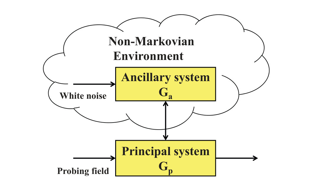 Figure 1
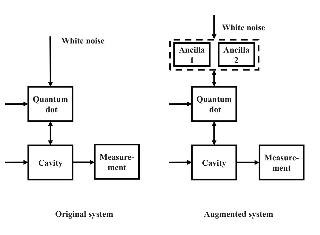 Figure 2
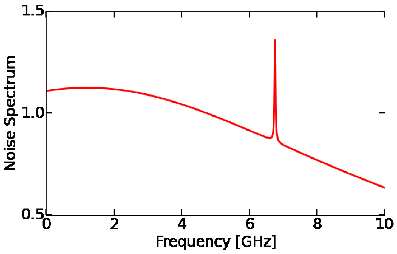 Figure 3
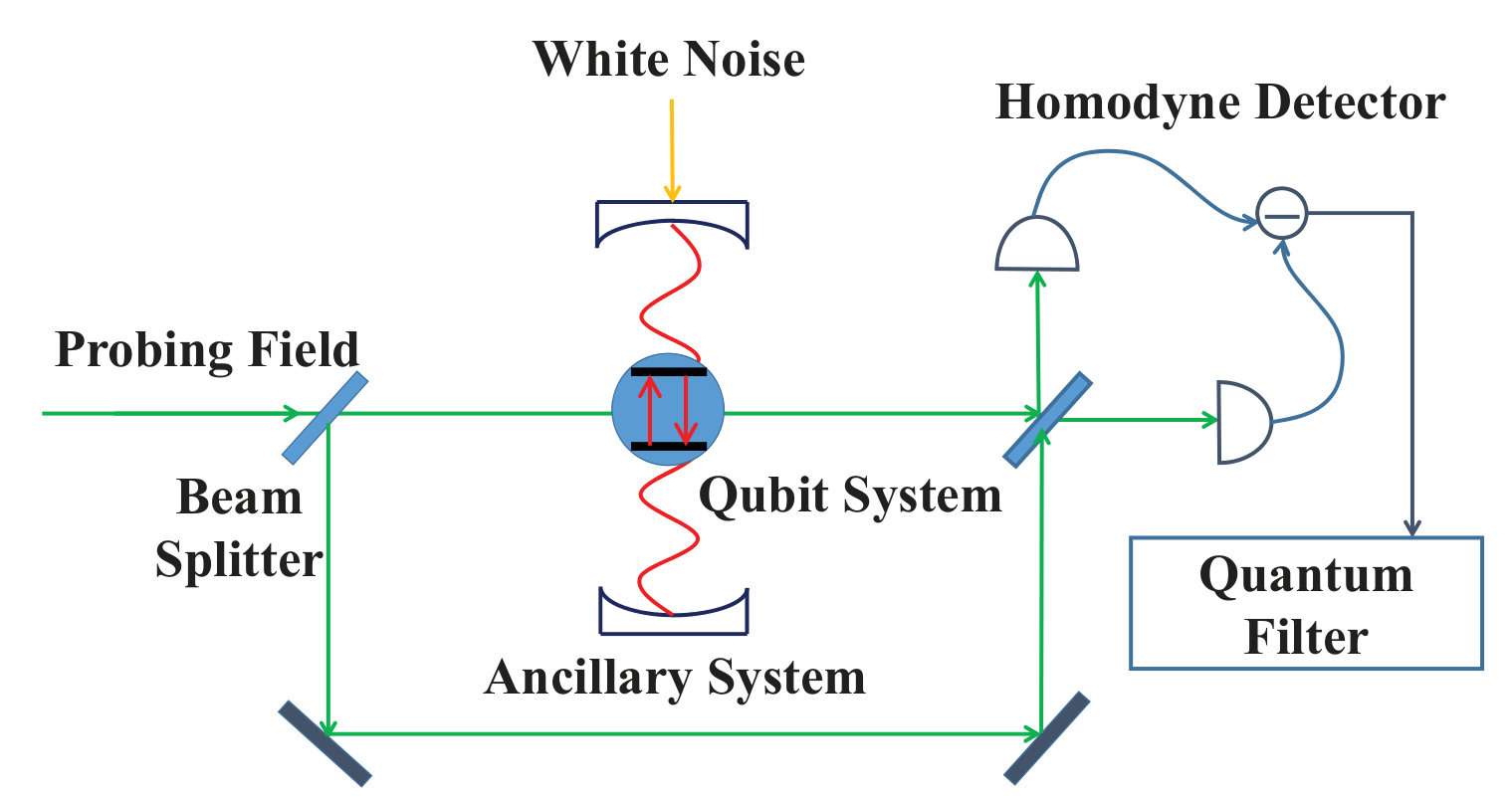 Figure 4
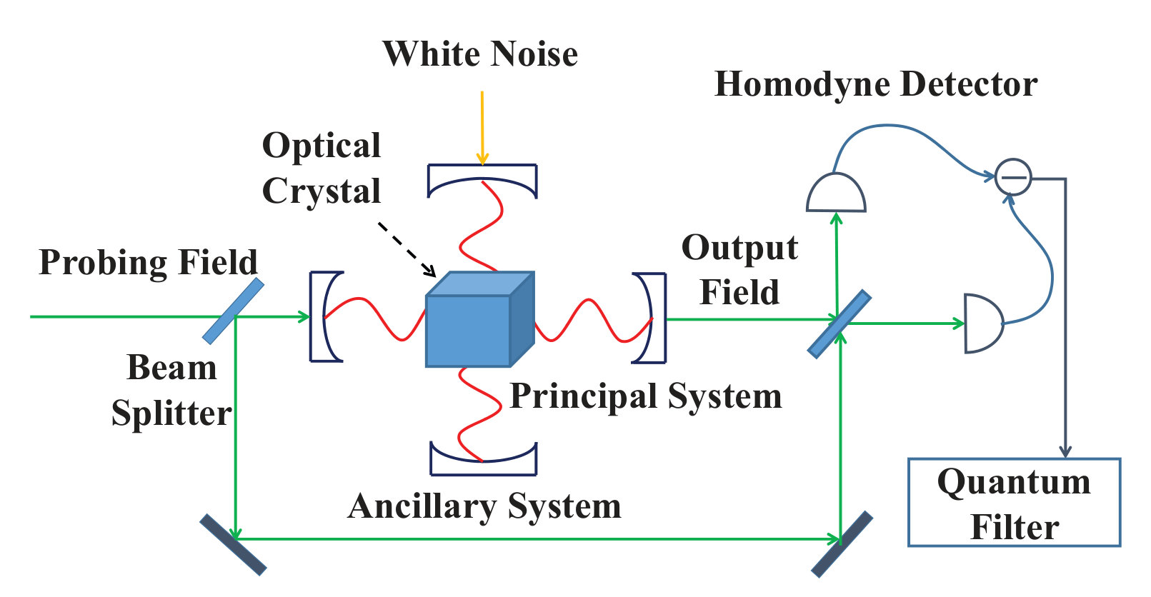 Figure 5
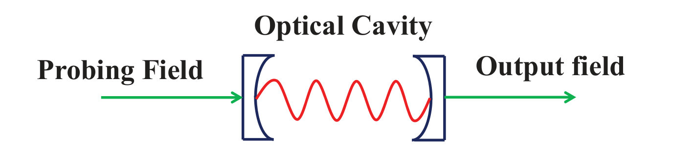 Figure 6
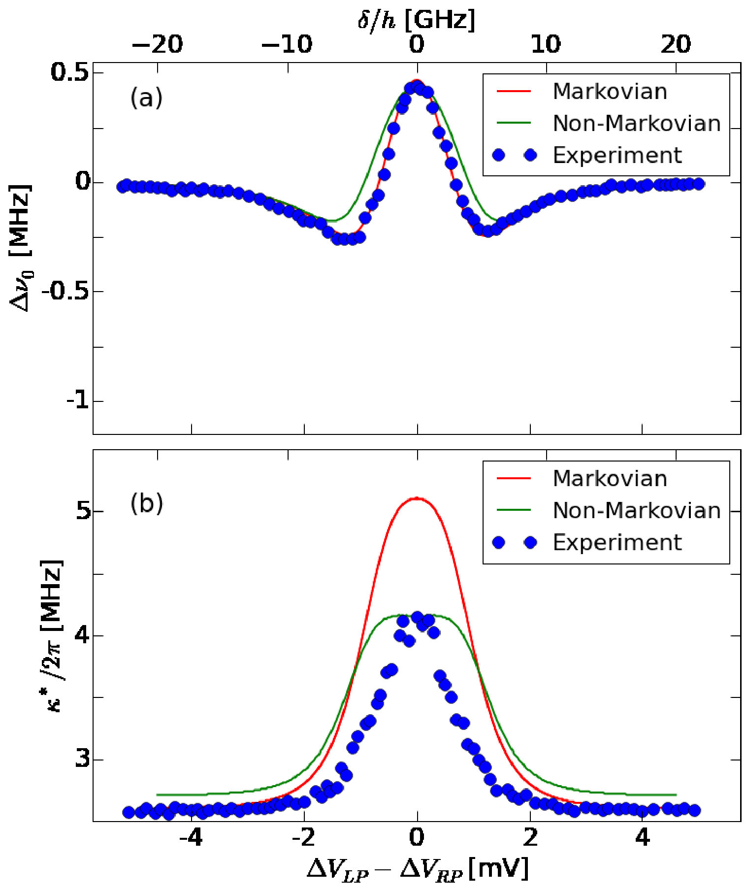 Figure 1
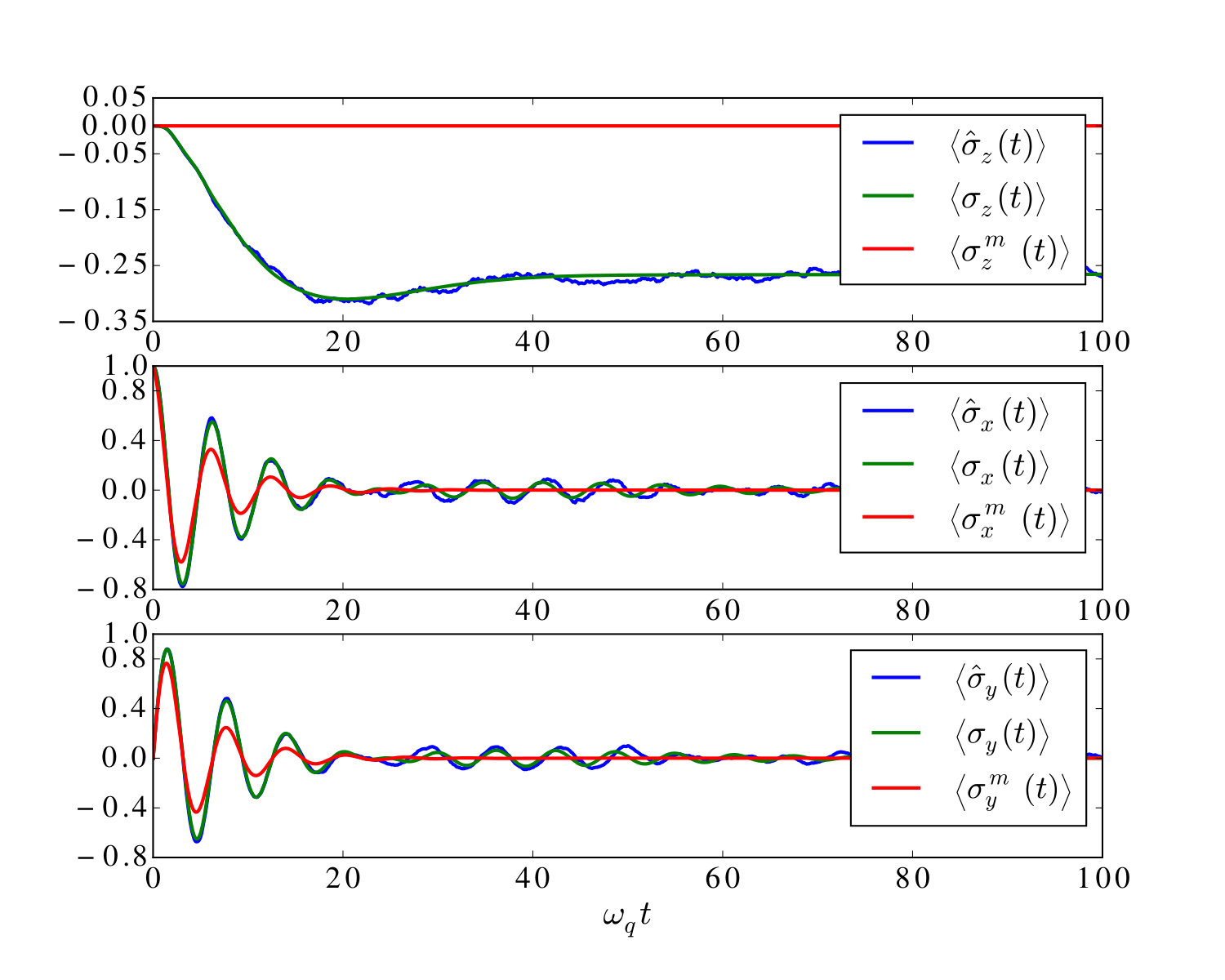 Figure 4
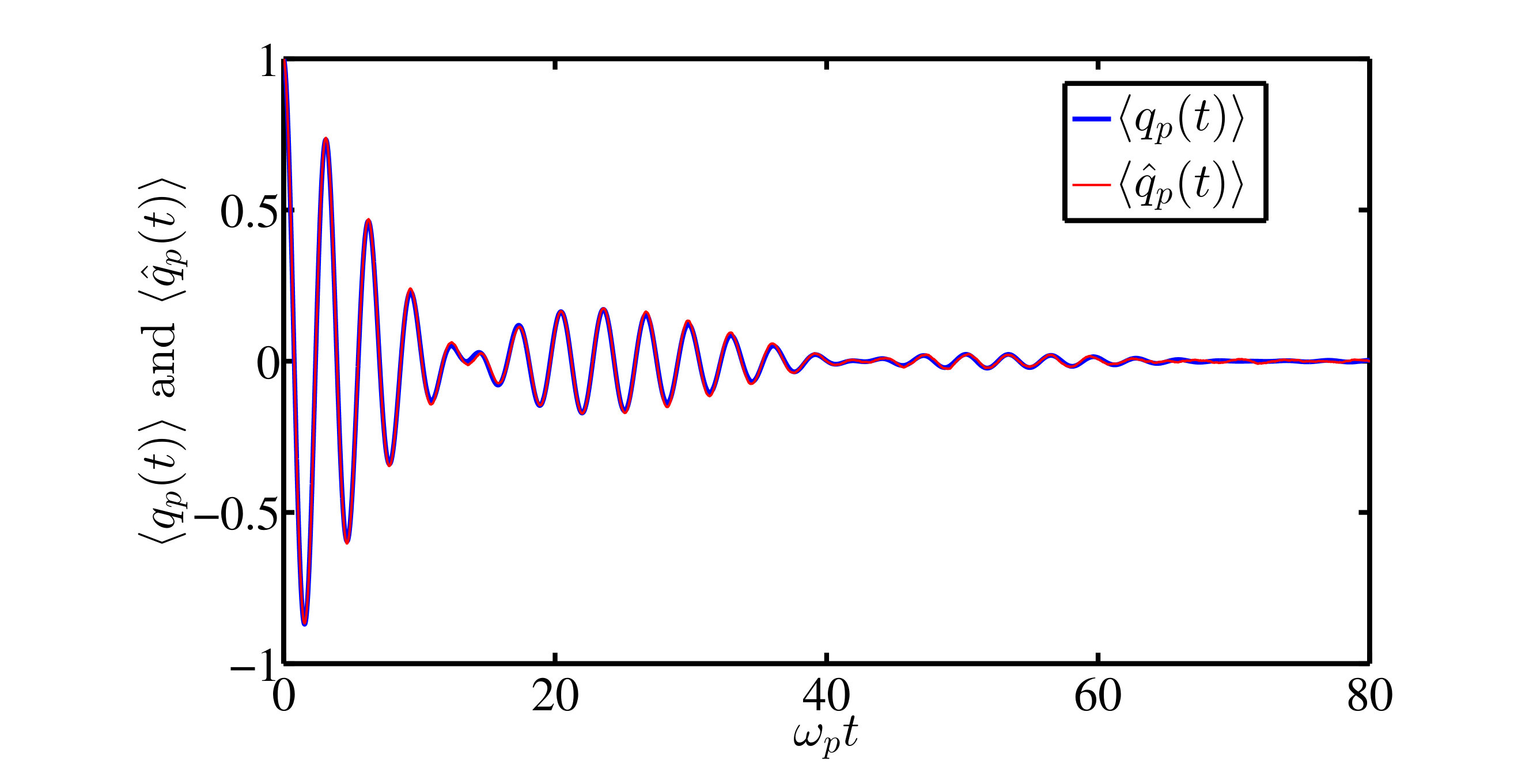 Figure 9
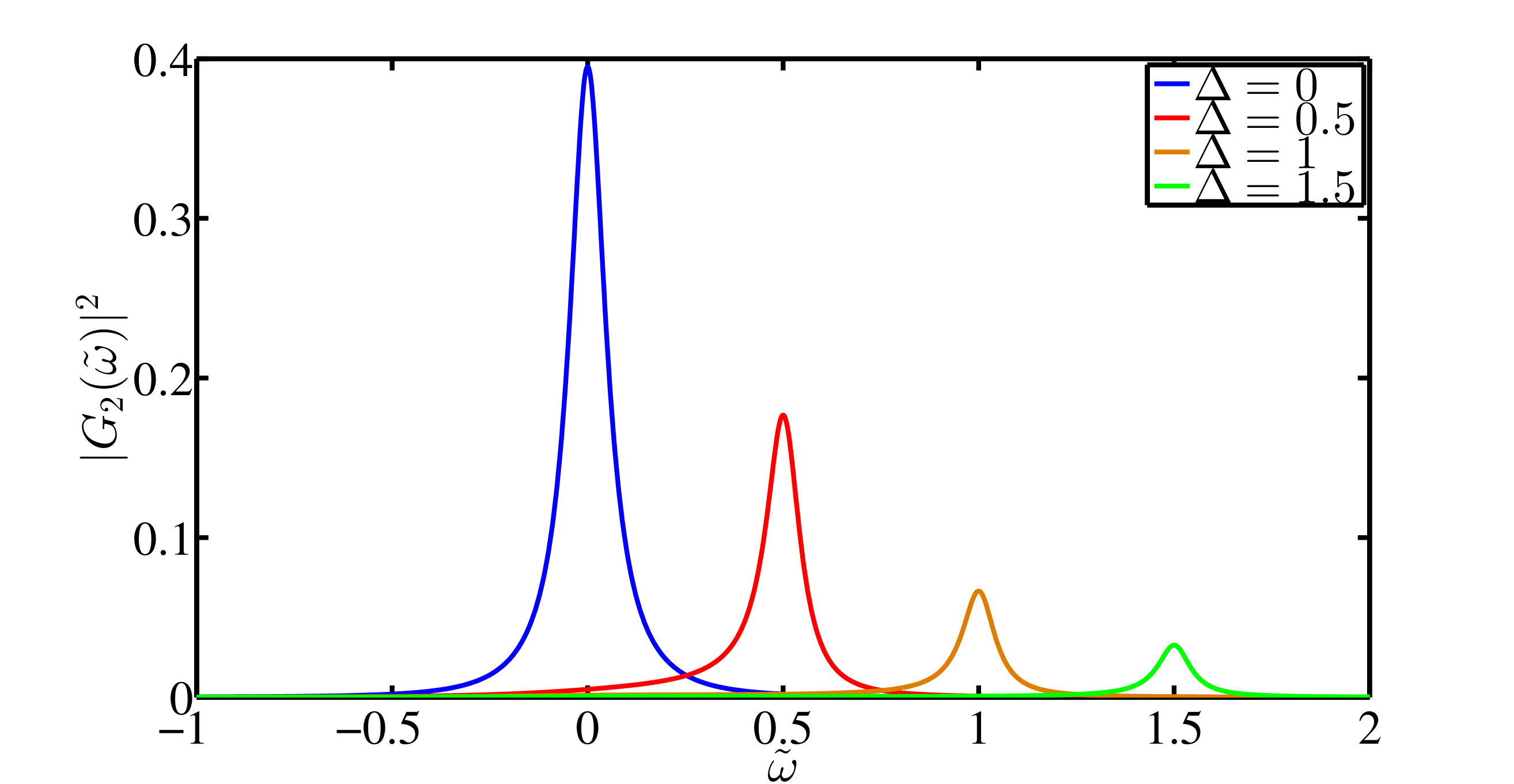 Figure 10
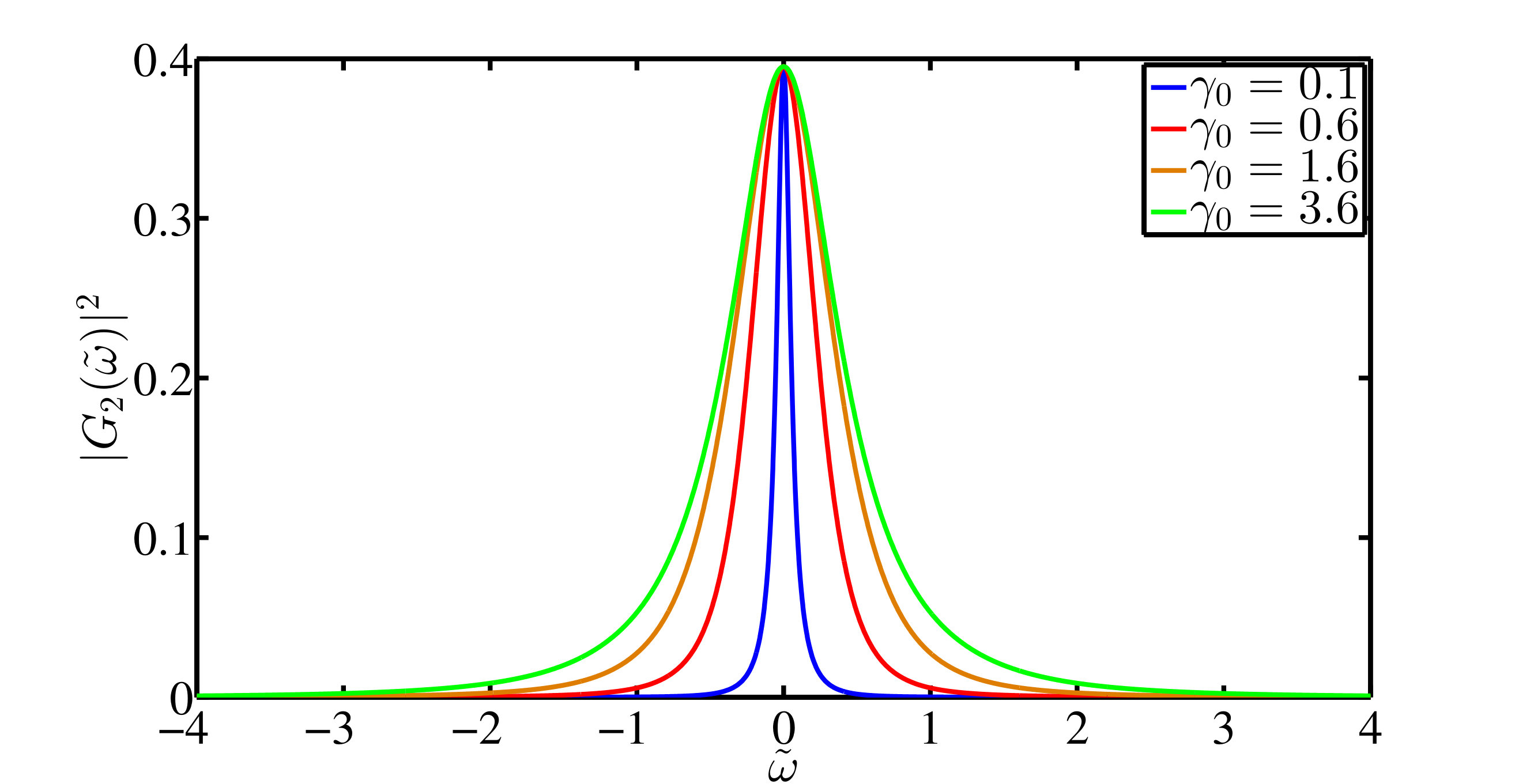 Figure 11
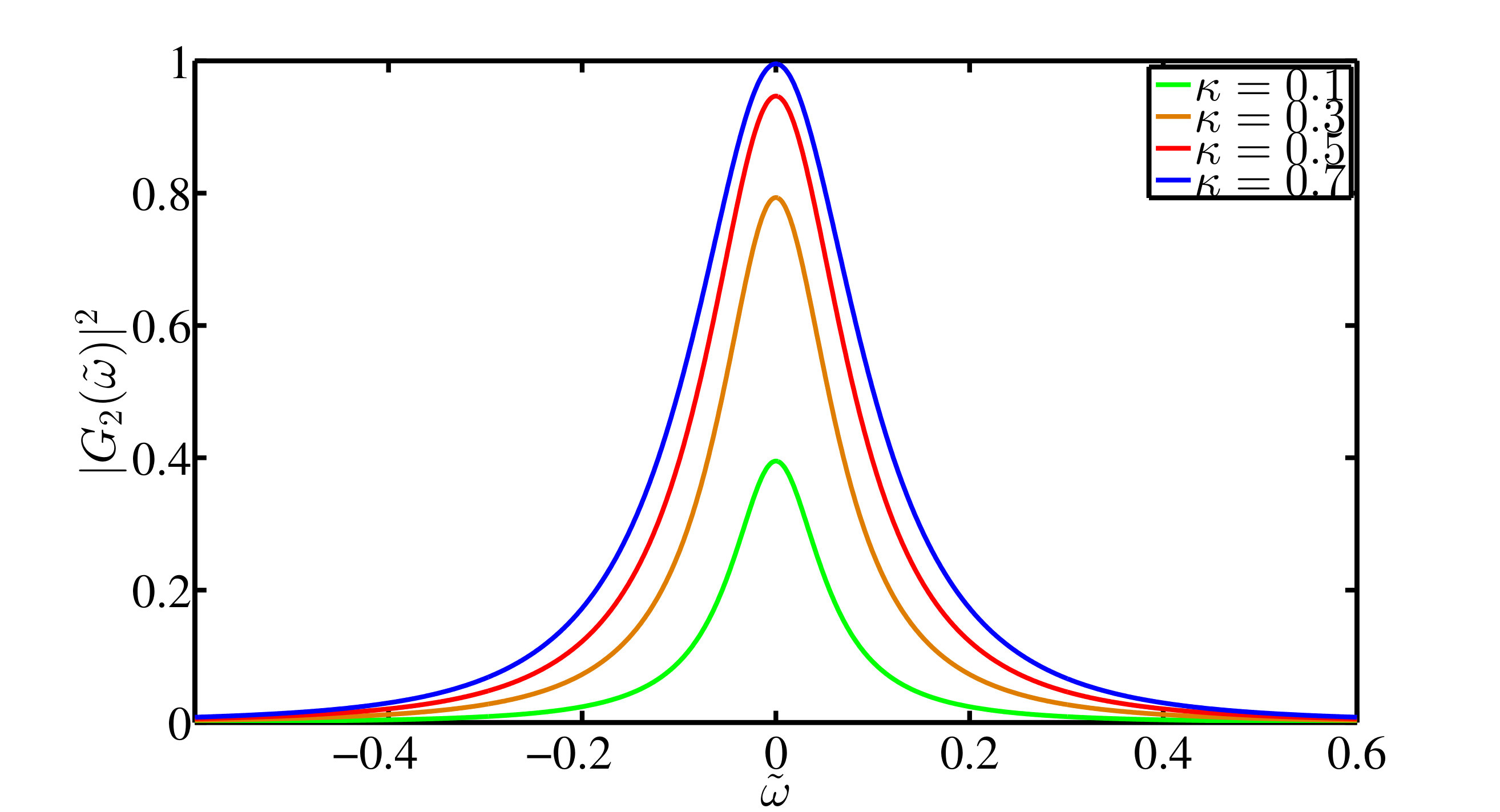 Figure 12
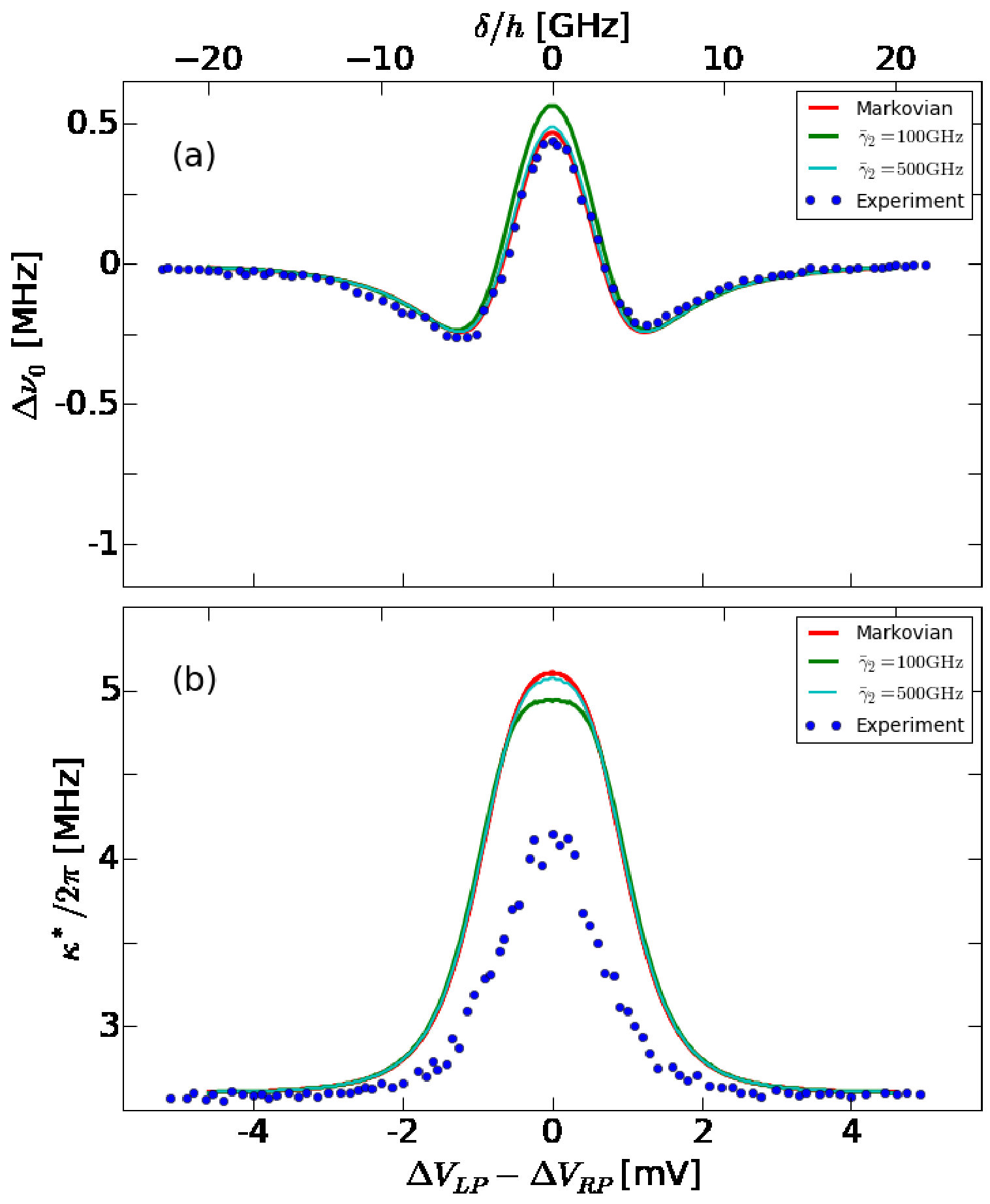 Figure 13
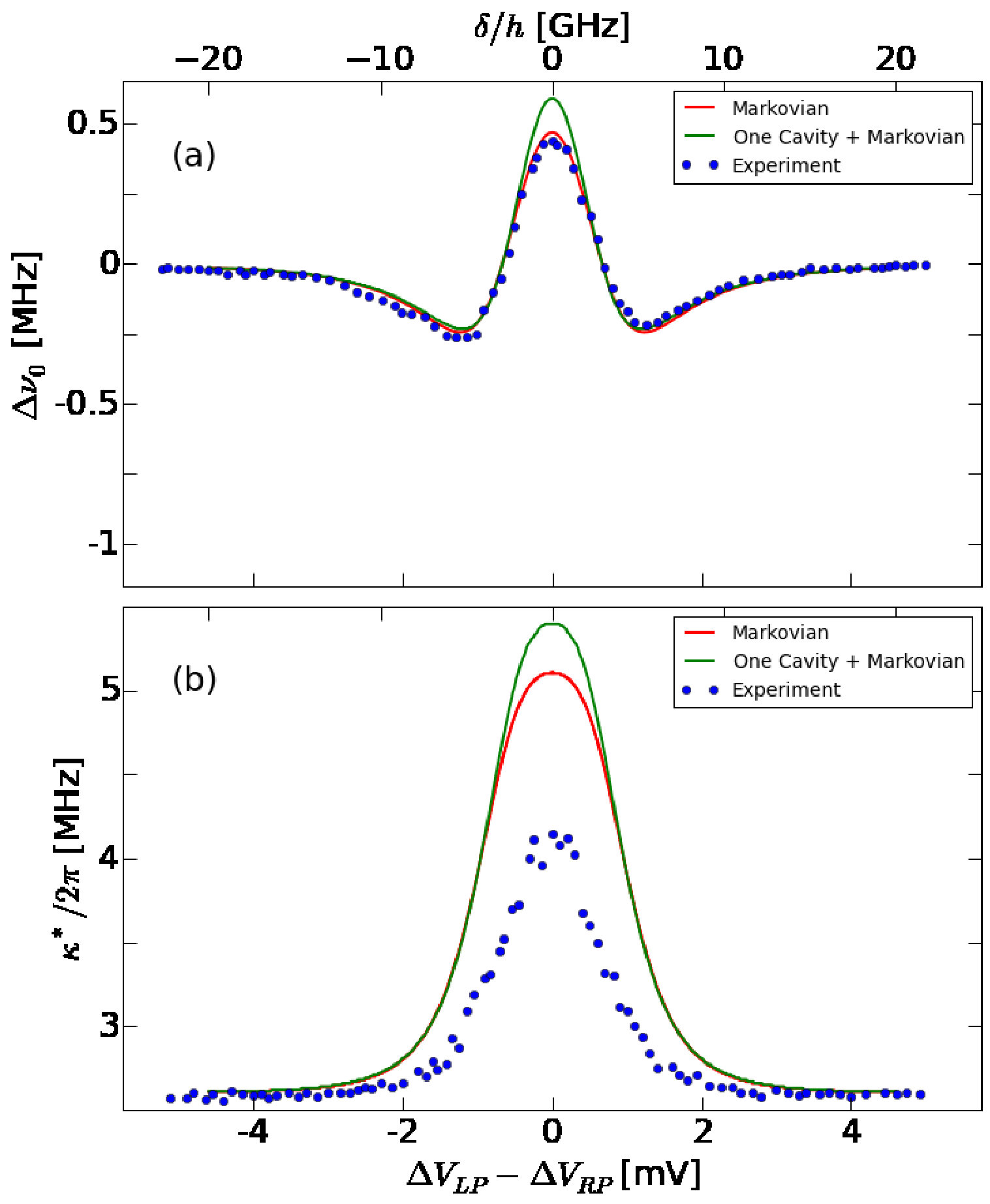 Figure 14
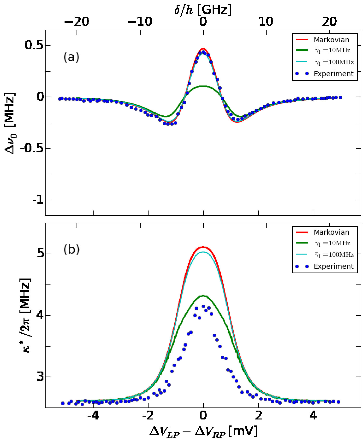 Figure 15
Peer Reviews
No public reviews on file for this paper yet. If you reviewed it on a platform where reviews are public (OpenReview, ICLR, NeurIPS, ICML), you can paste yours below so the community can read it here.
Videos
No videos yet. Explain this paper in a talk, walkthrough, or lecture? Add one.
Modelling and Filtering for Non-Markovian Quantum Systems
Shibei Xue [email protected]
Thien Nguyen [email protected]
Matthew R. James [email protected]
Alireza Shabani [email protected]
Valery Ugrinovskii [email protected]
Ian R. Petersen [email protected] School of Information Technology and Electrical Engineering, University of New South Wales at the Australian Defence Force Academy, Canberra, ACT 2600, Australia
Research School of Engineering, Australian National University, Canberra, ACT 2600, Australia
Quantum Artificial Intelligence Lab, Google, 340 Main St. Venice, CA 90291, U.S.A.
Abstract
This paper presents an augmented Markovian system model for non-Markovian quantum systems. In this augmented system model, ancillary systems are introduced to play the role of internal modes of the non-Markovian environment converting white noise to colored noise. Consequently, non-Markovian dynamics are represented as resulting from direct interaction of the principal system with the ancillary system. To demonstrate the utility of the proposed augmented system model, it is applied to design whitening quantum filters for non-Markovian quantum systems. Examples are presented to illustrate how whitening quantum filters can be utilized for estimating non-Markovian linear quantum systems and qubit systems. In particular, we showed that the augmented Markovian formulation can be used to theoretically model the environment for an observed non-Markovian behavior in a recent experiment on quantum dots [10].
keywords:
Non-Markovian quantum systems; Quantum stochastic differential equation; Whitening quantum filter; Quantum Kalman filter; Quantum colored noise.
††thanks: This paper was not presented at any IFAC meeting. This research was supported under Australian Research Councils Discovery Projects and Laureate Fellowships funding schemes (Projects DP140101779 and FL110100020), the Chinese Academy of Sciences President’s International Fellowship Initiative (No. 2015DT006), and the Air Force Office of Scientific Research (AFOSR) under agreement FA2386-16-1-4065. Corresponding author S. Xue, Tel. : (+61) 02-6268-9461
, , , , ,
1 Introduction
Control of open quantum systems has been rapidly advancing quantum information technology in recent years [5, 25, 33, 18, 29, 1, 8, 28], where an open quantum system refers to a quantum system interacting with an environment or other quantum systems.
Among open quantum systems, the most widely investigated class of quantum systems is that comprising quantum systems coupled with memoryless environment. Evolution of such systems can be described by master equations [5] in the Schrödinger picture and Langevin equaitons [5] or quantum stochastic differential equations [4] in the Heisenberg picture. Both mathematical models give rise to Markovian dynamics, thus this class of open quantum systems is commonly referred to as Markovian quantum systems. In addition, Markovian quantum systems can be coupled to a field satisfying a singular commutation relation, e.g., quantum white noise [12]. In terms of its stochastic description, the field has an independent increment over an infinitesimal time interval, which satisfies a non-demolition condition and can be measured to continuously extract information of the quantum system [3]. These properties of the environment are analogous to properties of a classical white noise and have served as a foundation for the well established quantum filtering theory aimed at estimation of Markovian quantum systems [4]. Such a theory underpins a number of successful control applications such the design of real-time feedback control laws for cooling a quantum particle [7], and stabilizing states [24] or entanglement [43, 47] of a quantum system.
However, many problems of interest involve more complicated environmental influences, which cannot be handled within the Markovian setting and require treating the environment as quantum colored noise. This necessitates the investigation of non-Markovian behavior of quantum systems [32, 40, 6, 39, 2, 38, 37]. A non-Markovian quantum system is a quantum system interacting with an environment with memory effects. To describe dynamics of non-Markovian quantum systems involving quantum colored noise, several models have been developed, for example, non-Markovian Langevin equations where non-Markovian effects are embedded in a memory kernel function [32] and time-convolutionless master equations where a time-varying damping function characterizes the non-Markovian damping processes [5], etc. However, these existing models for non-Markovian quantum systems are not compatible with the quantum filtering theory. In addition, unlike the quantum white nose, the quantum colored noise does not satisfy the singular commutation relations. For that reason, non-Markovian models are difficult to use for processing quantum measurements. Once the quantum colored noise is measured, the states of the quantum system interacting with this noise will be demolished.
A standard approach in classical control systems analysis and design is whitening of the colored noise by introducing additional dynamics so as to express the system with non-Markovian effects of colored noise as an augmented system model governed by a white noise. Thus a filter for the system involving colored noise can be constructed [19]; such filter is often referred to as whitening filter. Similar ideas have been explored for quantum systems as well. A pseudo-mode method was proposed for effectively simulating non-Markovian effects by using a Monte Carlo wave-function [15, 23], which was applied to model the energy transfer process in photosynthetic complexes [30]. Also, the dynamics of non-Markovian quantum systems can be described by using a hierarchy equation approach [21], which has been applied to indirect measurement of a non-Markovian quantum system [31]. An augmented system approach has been applied to obtain a quantum filter for quantum systems interacting with non-classical fields using a field-mediated connection method in a situation where the non-Markovian system does not introduce backaction on the environment [14].
In this paper we present a systematic augmented Markovian system approach to modelling non-Markovian quantum systems. To capture effects of the non-Markovian environment, we introduce ancillary systems to augment a principal system of interest, which are realized by linear open quantum systems. Compared to the principal system, the augmented system model is defined on an augmented Hilbert space. Also, we introduce a spectral factorization method to determine the structure of linear ancillary systems to ensure that its fictitious output has a power spectral density which is identical to that of the non-Markovian environment under consideration. Nevertheless, while these elements of our model follow the classical system modelling, the proposed model has a distinctively quantum feature in that the quantum plant and its non-Markovian environment mutually influence each other. This feature distinguishes quantum system-environment interactions from the classical case where the classical colored noise disturbs a plant but not vice versa [20]. To account for this special feature of non-Markovian quantum systems, in the proposed model the ancillary system is coupled to the principal system via their direct interactions rather than the field-mediated connection; cf. [14].
To describe the augmented Markovian system model for the non-Markovian quantum system, the paper adopts so-called description, where the internal energy, the couplings to the environment and the scattering process of the environmental field for a quantum system are captured by a Hamiltonian , a coupling operator , and a scattering matrix , respectively. An advantage of this approach is that it allows to describe system-environment interactions systematically using the formalism of quantum stochastic differential equations. To demonstrate this advantage and the utility of the proposed augmented Markovian modelling of non-Markovian quantum dynamics, we show how the proposed approach can be utilized to obtain whitening quantum filters for non-Markovian linear quantum systems and qubit systems. As an example application, this augmented Markovian model is utilized to explore quantum colored noise in a recent experiment for a hybrid solid-state quantum system [10].
The paper is organized as follows. In section 2, we briefly review a general description of Markovian quantum systems. Based on this description, an augmented Markovian system model is presented for non-Markovian quantum systems in section 3, where a spectral factorization method is proposed to obtain an ancillary linear quantum system model for a quantum environment with a given spectrum. Next, the application to derivation of a whitening quantum filter is presented in section 4 where examples of filters for linear non-Markovian quantum systems and single qubit systems are obtained. In section 5, an augmented Markovian system model is utilized to obtain an improved model for an experiment involving a hybrid solid-state system. Finally, conclusions and discussions are given in Section 6.
2 A brief review of the Markovian quantum system model
In this section, we will briefly introduce some standard facts about Markovian quantum systems. For more details, we refer the reader to references [11, 4].
2.1 Quantum white noise
In quantum physics, it is customary to describe an environment field as the Fourier transform of the annihilation operator of the field acting on the so-called Fock space [11]; that is
[TABLE]
The operator on the Fock space defined by (1) is called the quantum white noise field operator. It satisfies singular commutation relations
[TABLE]
where is the commutator of operators, i.e., for two operators and with suitable domain and image spaces. The symbol † denotes the complex conjugate of an operator.
The quantum white noise field can be interpreted as a quantum stochastic process. Associated with the field are an integrated operator , known as is a quantum Wiener process, and its adjoint . They satisfy the commutation relations [4]
[TABLE]
Under a common assumption that the initial state of the field is a vacuum field, the process is analogous to the standard Wiener process and the process is analogous to a Gaussian white noise with zero mean. For convenience, we summarize the Ito rules for the quantum infinitesimal increments of , in a vacuum state [11] which will be used in subsequent calculations,
[TABLE]
2.2 Quantum stochastic differential equation
Markovian quantum systems have been extensively investigated since they are suitable models for many physical systems. For example, optical modes trapped in a cavity (see Fig. 1) probed by a white noise field exhibit Markovian dynamics.
Markovian quantum systems can be described by quantum stochastic differential equations. Consider a Markovian quantum system and the associated triple characterizing its scattering matrix, the coupling operator and the Hamiltonian, respectively. In quantum mechanics, both the coupling operator and the Hamiltonian are represented as operators mapping an underlying Hilbert space into itself, As for the scattering matrix , from now on, we will assume since for simplicity the scattering process will not be considered here.
The unitary evolution operator of this Markovian quantum system is defined on the tensor product Hilbert space , it is known to satisfy the following quantum It stochastic differential equation
[TABLE]
In the Heisenberg picture, all quantum mechanical quantities of interest affected by the system evolution are operators that initially defined on the Hilbert space , and evolve on the Hilbert space . Specifically, an arbitrary operator defined on gives rise to the evolution of operators on the Hilbert space defined as . From (4), it follows that this evolution satisfies the quantum stochastic differential equation
[TABLE]
Here refers to the Lindblad generator [4]
[TABLE]
and the notation refers to the Lindblad superoperator defined as
[TABLE]
Quantum stochastic differential equations have been widely used in the analysis and control of Markovian quantum systems [4, 17, 42, 22].
2.3 Input-output relations
When a quantum white noise field passes through a quantum object and interacts with it, the resulting field is called an output field. It can be observed via measurement, e.g., homodyne detection [11]. Mathematically, the output field is described as . The quantum infinitesimal increment for the output field can be written as a quantum stochastic differential equation:
[TABLE]
which shows that the output field not only carries information about the quantum object but is also affected by the input noise. As a result, the output field can be utilized in estimating the dynamics of the quantum object [4, 44, 46].
2.4 Master equation
While this paper is exclusively setup in the Heisenberg picture, it is worth reminding about an alternative formulation known as the Schrödinger picture. In the Schrödinger picture, the state of a quantum system can be described by a wave function which is a complex vector in the Hilbert space . Based on the wave function , a trace class operator on is defined known as the density matrix of the quantum system [44].
In contrast to the Heisenberg picture introduced in the previous subsections, in which the operators evolve in time and the states are time independent, the states of a quantum system evolve in time while the operators are time independent in the Schrödinger picture. Of course, these two alternative representations of the quantum evolution are equivalent [5, 44].
The density matrix of a Markovian quantum system characterized by a triple and interacting with a quantum white noise obeys a so-called master equation
[TABLE]
where the adjoint of the Lindblad superopertor is calculated as .
3 An augmented model for non-Markovian systems
3.1 Preliminary remarks
A non-Markovian quantum system is a quantum system in an environment with memory, and is typically regarded as a quantum system disturbed by a quantum colored noise. In this paper we propose to model such environments as ancillary quantum systems excited by quantum white noise fields. This approach resembles the classical approach to modelling colored noise signals using shaping filters where the shape of the spectrum is related to internal modes of the filter. Similarly, in this paper we assume that the internal modes of the ancillary system correspond to dynamics of the non-Markovian environment. However different from the classical case, we show that the non-Markovian system behaviour and the system backaction on the environment can be explained using a direct coupling mechanism of environment-system interactions, within an augmented Markovian system picture.
This section begins with introducing a general framework for constructing such an augmented Markovian system model in Section 3.2. Next in Section 3.3, we show that the class of proposed augmented models is sufficiently rich in a sense that, given an environment with a rational power spectral density of its quantum colored noise, an ancillary linear quantum system model for this environment can be constructed to match that spectrum. This implies that a large class of non-Markovian environments can be modelled (exactly or with a sufficient accuracy) in terms of linear quantum systems consisting of quantum harmonic oscillators.
3.2 The general augmented Markov system framework
3.2.1 The description of the augmented Markovian
system model
Consider a quantum system operating in a non-Markovian environment. This system, which we call the principal system, has the following description
[TABLE]
where is the Hamiltonian of the principal system and is the coupling operator vector of the principal system with respect to a probing field defined on a Fock space . The operators and are defined on a system’s Hilbert space . Note that the coupling operator does not describe how the system is coupled with the environment, but allows the principal system to be probed for measurement, by shining an input field through probing channels and observing the output of the probing field so as to construct quantum filters.
The principal quantum system interacts with its environment by exchanging energy with the environment, i.e., they mutually influence each other. This energy exchange is captured by a direct interaction Hamiltonian
[TABLE]
where the operator vector describes the environmental effect, and is a coupling operator vector defined on the Hilbert space of the principal system.
In what follows internal modes of the environment are assumed to be stationary. Hence the quantum correlation matrix is independent of ; here denotes the quantum expectation defined as , where is the initial density matrix of the environment. Also the power spectral density characteristics of the environment can be defined in a standard fashion, as the Fourier transform of the quantum correlation function.
Definition 1**.**
The power spectral density of a stationary environment operator vector is defined as
[TABLE]
Note that since the definition of Fourier transform for quantum systems is actually the standard inverse Fourier transform but double sided Laplace transform in equation (11) is standard, we have .
It is straightforward to verify using singular commutation relations that when is the quantum white noise and the environment is Markovian, then . On the other hand, when defined by equation (11) is not equal to 1, this corresponds to a colored noise .
To model internal modes of the environment, we introduce an ancillary Markovian quantum system with a Hamiltonian operator and a collection of coupling operators with respect to ancillary quantum white noises, combined into a coupling operator vector . Using the compact notation, such an ancillary system is denoted
[TABLE]
as noted previously, the scattering matrix is assumed to be identity. Note that the ancillary system evolves on a Hilbert space , where the ancillary system and the corresponding white noise are defined on the Hilbert space and the Fock space , respectively. Also associated with this system is a vector of operators of the ancillary system defined on the Hilbert space . This vector of operators represents the quantum colored noise whereby the ancillary system interacts with the principal system; see (10). As the ancillary system is driven by a quantum white noise, it can be thought of whitening the quantum colored noise arising from the non-Markovian environment.
The general quantum feedback network theory [13] can now be applied to describe interactions between the principal system and the environment. From this theory, the combined system model representing the principal quantum system and the ancillary system model (12) for the non-Markovian environment interacting via the Hamiltonian (10) has the following parameters,
[TABLE]
A schematic diagram of the augmented system is shown in Fig. 2. The augmented system is defined on the tensor product Hilbert space . Since this augmented system only interacts with quantum white noise fields, namely with the ancillary white noise field and the probing field, the overall system is Markovian. However, as we will show in the next section, the principal subsystem is not Markovian due to the interaction with the ancillary system.
3.2.2 Quantum stochastic differential equations for the augmented
system
By substituting (13) into (4) the Heisenberg picture stochastic differential equation of the evolution operator for the augmented system (13) can be obtained to be
[TABLE]
Here, and are the quantum infinitesimal increments for the noise processes of the principal and ancillary system, respectively. Then using (14), the evolution of an augmented system operator can be defined as which satisfies the quantum stochastic differential equation
[TABLE]
where and other time-varying operators are obtained in the same way as .
Note that any operator of the augmented system can be written as , i.e., a tensor product of a principal system operator and an ancillary system operator . Thus, the generator for the augmented system can be expressed as
[TABLE]
where
[TABLE]
are the generators for the principal system and the ancillary system, respectively.
In particular, for , i.e., a principal system operator, Eq. (3.2.2) reduces to
[TABLE]
with . When , i.e., an operator of the ancillary system, we have
[TABLE]
with . Note that in quantum mechanics it is conventional to write and as and , respectively.
One can see form (3.2.2) that due to the direct coupling term induced by the ancillary system in the second line of Eq. (3.2.2), the principal system will not behave as a Markovian quantum system when it is coupled with the ancillary system. Indeed, the ancillary system operator can be treated as an input into the principal system generated by the ancillary system. As we noted earlier this input represents a colored noise generated by the environment, which explains a non-Markovian nature of the principal systems dynamics. Also, it can be seen from (3.2.2) that the evolution of the ancillary system operator depends on the principal system operator , which shows that the principal system acts back on the ancillary system. This explains the non-Markovian behaviour of the environment.
3.2.3 A master equation for the augmented system
Alternatively, dynamics of the augmented system can be described using a master equation. In particular, it is convenient to use master equations when the principal system is a qubit system involving nonlinear dynamics. This will be shown in section 5.
For the augmented system (13), the master equation (8) takes the form
[TABLE]
where is the density matrix of the augmented system. Once again we observe that the state evolution of the augmented system is Markovian, since future values of the density matrix only depend on the present density matrix. One can also obtain the density matrix of the principal system as the partial trace with respect to the ancillary system,
[TABLE]
3.3 Linear quantum systems models for non-Markovian
environments with rational power spectral densities
We now demonstrate that the proposed modelling of non-Markovain systems is sufficiently rich in a sense that for a broad class of environment power spectral densities , an ancillary system can be constructed whose characteristics match . Specifically, we show that when the environment has a rational power spectral density, the corresponding ancillary system can be realized within the class of linear quantum systems. Clearly, when is not rational, but can be approximated by a rational power spectral density, an approximating ancillary linear quantum system model can be constructed. From a practical perspective, such an approximation is often sufficient and leads to meaningful results as will be demonstrated in Section 5.
First, let us consider a linear quantum system comprised of harmonic oscillators interacting with channels of quantum white noise fields and obtain an expression of the associated power spectral density. Since our aim is to represent a non-Markovian environment in a form of an ancillary system and such environments do not generate energy, we restrict attention to the class of linear quantum systems whose quantum stochastic differential equations only involve annihilation operators.
To obtain an expression for the power spectral density of a linear annihilation only system, we begin with its description. Specifically, the Hamiltonian of such a linear system has the form
[TABLE]
where is a column vector of annihilation operators with an annihilation operator as its -th component, and is the corresponding row vector of creation operators. These operators are defined on the common Hilbert space and satisfy the singular commutation relations
[TABLE]
The diagonal and non-diagonal elements of the Hermitian matrix represent the internal angular frequencies and the couplings between the harmonic oscillators, respectively. Also, the system is coupled with a white noise field, and the corresponding coupling operator of such a linear annihilation only system with respect to the quantum white noise fields can be expressed as
[TABLE]
with a matrix . Also, according to our standing assumption, the identity scattering matrix is assumed.
With these Hamiltonian and coupling operators, the evolution operator of the linear ancillary system satisfies
[TABLE]
where is the quantum infinitesimal increment for the white noise field process. Then, the annihilation operators of the system evolve according to the linear quantum stochastic differential equation
[TABLE]
where and .
Our result concerning the modelling of a colored noise environment in terms of linear systems of the form (27) is summarized in the following theorem. Since non-Markovian quantum systems normally involve only one kind of colored noise, for simplicity we restrict attention to single input ancillary systems; that is, and the corresponding spectral density is scalar. The extension to the matrix case is quite trivial, as will be seen from the proof.
Theorem 2**.**
Suppose that the power spectral density of an environment colored noise process is rational and satisfies for all . Then there exists a linear quantum system in the form of (27) and a matrix , such that the process
[TABLE]
has the desired power spectral density .
Note that although the operator (28) is expressed in terms of operators of the system (27), unlike the input defined in Eq. (7) it is not an output field of the system available for quantum measurement. Yet it represents a physical quantity whereby the ancillary system can interact with other quantum systems.
The proof of Theorem 2 will be given later in this section. Before proving the theorem, it is instructive to compute the power spectral density of the operator (28). Since the system (27) is to represent internal modes of the environment, its dynamics can be assumed to start from a long time ago. Formally, this means that the initial time when the system (27), (28) was at rest is . Hence, can be expressed as
[TABLE]
where
[TABLE]
is the inverse Laplace transform of the transfer function matrix
[TABLE]
That is, is analogous to the stationary response of a linear system with the transfer function matrix to a white noise input.
The covariance of can be found using the quantum Ito calculus rules. Assuming that (the case is treated in the same way), we obtain
[TABLE]
The last integral vanishes since the time intervals do not overlap and thus we have
[TABLE]
Using Definition 1, its power spectral density can be computed to be
[TABLE]
where is the adjoint of the transfer function . The calculation is analogous to the calculation of the power spectral density for an output of a classical linear system driven by a white noise input [19].
It follows from (32) that the spectral factorization method can be employed to obtain a linear quantum system representation of the environment with a positive rational spectral density .
Proof of Theorem 2
Given a power spectral density , we will determine the corresponding Hamiltonian (23) and the coupling operator (25) which define the linear quantum system (27), (28). First we observe that according to [35, Theorems 5, 7], can be factorized as in (32) with a stable transfer function
[TABLE]
Next, a stable transfer function of the form (33) has a state-space realization with matrices
[TABLE]
i.e., ; e.g., see [19]. Since such a realization is Hurwitz and controllable, the Lyapunov equation
[TABLE]
for this realization has a unique and invertible solution [19]. Hence, we can find a factorization for the inverse of , i.e., and thus equation (45) can be reexpressed as
[TABLE]
Define
[TABLE]
and substituting this notation into (46):
[TABLE]
This equation shows the new realization (47) obtained from (42) by applying the coordinate transformation satisfies the physical realizability condition of [22]. Also, it follows from [22] that we can obtain expressions for the Hermitian matrix and the coupling operator as
[TABLE]
These quantities define the system (27) as a linear quantum system.
As an example, let us particularize the result of Theorem 2 for the Lorentzian power spectral density of the form
[TABLE]
which commonly arises in solid-state systems [48, 34].
Corollary 3**.**
The power spectral density (50) of the Lorentzian noise can be realized by a single mode linear quantum system
[TABLE]
with the annihilation operator .
{pf}
The Lorentzian spectrum (50) can be factorized as in (32) with
[TABLE]
The order of the denominator of this transfer function is one, i.e., , which means the ancillary system can be realized by a single mode linear quantum system. Then, the matrices , , and reduce to scalars. From (42), we obtain
[TABLE]
Substituting (53) into the Lyapunov equation (46), we have , which can be solved to give
[TABLE]
According to (47), the realization of the system (27) with
[TABLE]
satisfies the physical realizability condition (48). Hence, equation (51) corresponds to a physically realizable linear quantum system. Indeed, from (49), the Hamiltonian and the coupling operator of this system can be obtained
[TABLE]
where is the annihilation operator of the system.
Remark 4**.**
The central frequency of the Lorentzian power spectral density (50) determines the angular frequency of the ancillary system, and the bandwidth of the power spectral density determines the system damping rate with respect to the white noise field.
4 Application to quantum filtering
4.1 Whitening quantum filter for non-Markovian quantum systems
In quantum physics, to force a quantum system to generate an output field, it must be excited with a probing field. Typically, such a filed is a quantum white noise field, . The quadrature of the output field,
[TABLE]
can be monitored via homodyne detection, and the measurement results can be utilized to construct a filter for the system. In this section we show that when the probing field is applied to a principal system directly interacting with an ancillary system, an augmented-system-based quantum filter, i.e., a whitening quantum filter can be derived to process measurements of the output field. Our derivation is based on the following assumptions regarding the physical apparatus.
Assumption 5**.**
The probing field is a quantum white noise field in a vacuum state, which satisfies a non-demolition condition such that the dynamics of the augmented system can be continuously monitored **[4]**. 2. 2.
The monitored channels are assumed to be coupled with the principal system via the operator . 3. 3.
The homodyne detector is perfect with detection efficiency.
Definition 6**.**
The quantum filtering problem is to determine an estimate of an observable which is the conditional expectation
[TABLE]
i.e, the projection of on , the commutative subspace of operators generated by the measurement results .
By applying the existing quantum filtering theory, we immediately obtain the whitening filter for the augmented system derived in Section 3.
Theorem 7**.**
Under the Assumption 5, a quantum filter for the augmented system can be constructed as
[TABLE]
The measurement process induces an innovation process satisfying
[TABLE]
and whose increment is independent of , .
{pf}
This whitening filter can be derived by applying the standard orthogonal projection approach developed in [4, 3] to the augmented system model .
Our next result concerns estimating the density matrix of the augmented system.
Definition 8**.**
The conditional density matrix of a quantum system is a density matrix which satisfies the equation
[TABLE]
Remark 9**.**
According to the above definition, the conditional density matrix is a density matrix for which the quantum expectation of in the Schrödinger picture coincides with the orthogonal projection of onto the commutative subspace .
Theorem 10**.**
The conditional density matrix for the augmented system satisfies the stochastic master equation
[TABLE]
with
[TABLE]
where the superoperator is the adjoint of .
{pf}
The stochastic master equation for the conditional density matrix defined in (59) can be derived from the whitening quantum filter (58) by using the methods in [4, 3].
In practice, when one is interested in estimating the principal non-Markovian system, it is the conditional density matrix of the principal system that will be of interest. Formally, it can be obtained as the partial trace of , by tracing out the ancillary system
[TABLE]
Earlier in Section 3.3 we have proposed representing ancillary systems using linear quantum systems. In this case, equation (62) reduces to where the number of bases for the linear quantum system is infinite. This makes obtaining an exact expression for from (62) rather difficult. However, approximating the linear ancillary system with a -level system will have an effect of truncation, and thus it is possible to calculate an approximation to the partial trace (62) [1].
4.2 Whitening quantum filter for linear non-Markovian quantum
systems
In this section, we consider the case where the principal system is a linear quantum system whose description involves only annihilation operators. For such quantum systems, we show that the whitening quantum filter is actually a quantum Kalman filter.
As noted previously, the Hamiltonian of a linear annihilation only principal system is quadratic and can be expressed as
[TABLE]
where is a column vector of annihilation operators for the principal system. Also as before, is the corresponding row vector of creation operators for the principal system. These operators satisfy the singular commutation relations, cf. (24):
[TABLE]
The diagonal and off-diagonal elements of the Hermitian matrix are determined by the angular frequencies of components of the principal system and their couplings, respectively.
Also, the coupling operator with respect to channels of the quantum white noise process and the direct coupling operator are specified as
[TABLE]
respectively, where and .
As described in the previous section, the system interacts with a non-Markovian environment. These interactions can be captured using a model where the principal system is directly coupled with a linear ancillary system. Thus, the quantum stochastic differential equation for the augmented system including both the principal and the ancillary systems can be obtained
[TABLE]
where and . Also, the output field excited by the probing the principal system with the white noise filed process is
[TABLE]
with .
Suppose that the position quadrature of the output,
[TABLE]
is observed via homodyne detection. Also, since the operators in Eqs. (77) and (78) are not self-adjoint and the coefficients may be complex valued, it is convenient to transform Eqs. (77) and (78) into a phase space in terms of position and momentum operators as
[TABLE]
with , ,
[TABLE]
where
[TABLE]
are the quadrature representations of the operators of the principal and ancillary systems and the probing and quantum white noise fields, respectively. The components of and are calculated by applying the coordinate transformation matrix \Pi=\frac{1}{\sqrt{2}}\left[\begin{array}[]{cc}\rm I&\rm I\\ -{\rm i}\rm I&{\rm i}\rm I\\ \end{array}\right] to the corresponding components of the vectors of annihilation operators of the principal and ancillary systems:
[TABLE]
Note that the noise processes and are correlated, and the covariance matrix of is , where
[TABLE]
We are now in the position to present the whitening quantum filter for computing the estimate of the vector of dynamical variables of the linear augmented system model (79).
Theorem 11**.**
The whitening quantum filter for the linear augmented system (79) is a steady-state quantum Kalman filter
[TABLE]
with the Kalman gain
[TABLE]
obtained from the solution of the algebraic Riccati equation
[TABLE]
This theorem is obtained by applying the existing quantum Kalman filtering results for linear quantum systems [16, 41] to the linear augmented Markovian system (79). The obtained whitening quantum filter is driven by the output . Note that the symmetrized covariance matrix is independent of the measurement process.
4.3 An illustrative example: A non-Markovian optical system
The system
In this example, we consider a single mode non-Markovian bosonic quantum system disturbed by Lorentzian noise, which can be realized by two coupled cavities as shown in Fig. 3. In this figure, the horizontally oriented cavity is the principal system to be estimated. The vertically oriented cavity is the ancillary system converting white noise to Lorentzian noise. The optical modes in the two cavities are directly and strongly coupled by an optical crystal. A probing field is applied to the principal cavity, whose output is observed via homodyne detection. These measurements are used as the data for a quantum filter.
The Hamiltonian operators of the principal and ancillary cavities are and , respectively, with angular frequencies and . They are expressed in terms of respective annihilation and creation operators , and , satisfying the corresponding singular commutation relations (64) and (24). Then, the coupling operators of the principal cavity and are specified to be and , with constant , . Also, the coupling operator of the ancillary system with respect to the white noise is . The cavities interact through the operators and ; see (10). With these definitions, the quantum stochastic differential equations for the augmented system can be expressed in the of form (79)
with matrices
[TABLE]
The corresponding operators and in this example are the quadrature representations of the operators of the principal and ancillary systems and the probing and quantum white noise processes, respectively:
[TABLE]
Note that is the position quadrature of the output of the probing field process.
Whitening filter estimates vs the mean of the principal system
Assume the initial state of the augmented system is Gaussian [27] and thus, the mean of the system operators satisfying can serve as an estimate of the system dynamics; here the quantum expectation is with respect to the initial quantum state , . On the other hand, the estimates conditioned on the homodyne detection data are generated by the quantum Kalman filter (86). We now compare these estimates.
We choose the parameters of the system as , , , and and assume that the initial mean of the unconditional dynamical variables is the same as the initial conditional expectation for the quantum Kalman filter, i.e., where the first element of is . In Fig. 4, the red line is the trajectory of the mean of the unconditional position operator for the principal system. The oscillations of the curve envelopes are caused by the disturbance of the ancillary system, which indicates that energy is exchanged between the principal and the ancillary system showing non-Markovian characteristics. Compared with the unconditional trajectory, the blue line in Fig. 4 shows the average trajectory of the conditional expectation of the position obtained by averaging over 10000 realizations. It matches the red line very closely. This shows that on average, the whitening quantum filter estimates dynamics of the unconditional variable of the principal system.
The spectrum with respect to the white noise field
Generally, the output field spectrum is indicative of properties of the system. To calculate the power spectral density of the output of the probing field, we recall the quantum stochastic differential equation of the augmented system
[TABLE]
where and are the probing field and ancillary white noise field processes, respectively. The output equation with respect to the probing field is
[TABLE]
By detecting the position quadrature of the output field , the power spectral density of the output field can be calculated to be
[TABLE]
where , and and are the transfer functions from the probing field process and the quantum white noise process to the output field process, respectively. The square of their norms are expressed as
[TABLE]
with , .
Although the total output spectrum given in (106) is flat due to the passivity properties of the system [45], we can apply a coherent probing field whose strength is much higher than the strength of the ancillary quantum white noise and thus the spectrum can be observed. This allows us to calculate the spectrum which reflects the influence of the ancillary system on the output field.
Fig. 5(a) shows the power spectral density varying with the coupling strength . Here, we assume that there is no detuning (i.e., ) and the damping rates of the principal system to the probing field and of the ancillary system to the quantum white noise field are and . As the coupling strength is increased, the amplitude of the noise spectrum is increased, which means that the disturbance for the principal system becomes stronger.
The power spectral density varying with the detuning is plotted in Fig. 5(b) with parameters , and . When there is no detuning, the noise is strong at the system frequency, as the blue line shows. As the detuning is increased via decreasing the angular frequency of the ancillary system, the spectrum is driven away from the system frequency, and its amplitude is reduced as well. This illustrates that the non-Markovian effect generated by the ancillary system becomes weaker as the detuning is increased. When the detuning is large enough, the dynamics of the ancillary system become negligible. This is consistent with the results in [7].
Fig. 5(c) shows the power spectral density varying with the damping rate . As predicted, the bandwidth of the Lorentzian spectrum is broader as increases.
4.4 Quantum filter for a non-Markovian single qubit system
A qubit is a basic unit of quantum information, and is defined on a two-dimensional complex Hilbert space spanned by the Pauli matrices [26]
[TABLE]
In addition, the ladder operators for the qubit system
[TABLE]
are utilized to describe a state flip between the ground state and the excited state . The ladder operators can also be used to describe the interaction with external systems, e.g., in the Jaynes-Cummings model [36].
The Hamiltonian of the single qubit system we consider is given as
[TABLE]
where is the qubit working frequency characterizing the energy difference between the ground state and and the excited state.
A non-Markovian qubit system can also be represented as an augmented system (13), where the Hamiltonian of the principal system is replaced by and the coupling operator and the direct coupling operator are defined on the Hilbert space . Thus, we can write down a quantum filter for the qubit system in the Heisenberg picture as Eq. (58). However, these filter equations are infinite dimensional. Hence, for a non-Markovian qubit system, it is useful to calculate the evolution of the unconditional and conditional states in the Schrödinger picture using the master equation (21) and the stochastic master equation (60), respectively.
As an example, consider a single qubit system disturbed by Lorentzian noise arising from an ancillary system as shown in Fig. 6. As in the previous section, the ancillary system is a single mode linear quantum system with the Hamiltonian , the coupling operator , and the fictitious output . Here, the damping rate of the ancillary system with respect to the quantum white noise field is . In addition, the qubit is coupled with the ancillary system and the probing field through the direct operator and the coupling operator , respectively, with the direct coupling strength and the damping rate of the qubit ., The single qubit system is initialized in a state , where is the density matrix of the qubit and is the identity matrix. The angular frequency of the ancillary system is equal to that of the qubit, . Note that the dynamics of the ancillary systems cannot be eliminated via the adiabatic elimination which is only valid for the off-resonant case, i.e., when there exists a large detuning between the qubit system and the ancillary systems [7].
Fig. 7 shows the evolution of both the unconditional and averaged conditional expectation values of the observables , , and for the non-Markovian qubit system. The conditional state for the augmented system can be obtained from the quantum filter (60) and thus the conditional expectation of the observables for the qubit system can be calculated as , where . Here, is the identity matrix defined on the Hilbert space of the ancillary system. The averages of the three conditional expectations , and are plotted as blue lines; they are obtained by averaging over 500 realizations of the trajectories. The green lines represent the unconditinal expectations , and which are obtained from the master equation for the augmented system (21). Once again, we observe that the whitening quantum filter can estimate the non-Markovian evolution of the single qubit system.
To compare with the non-Markovian trajectories, the unconditional expectation values of the observables , , and for the qubit system in the Markovian case are also plotted as the red lines in Fig 7, where the qubit is directly open to the quantum white noise field and the probing field. In this case, the system dynamics obey a Markovian master equation
[TABLE]
The comparison shows that not only does the qubit in the Markovian case damp faster than that in the non-Markovian case but also the stationary states of the qubit in the two cases are different.
5 Application to an experiment on a hybrid solid-state quantum device
In some experiments involving solid-state systems, Markovian system models cannot completely explain some subtle phenomena. For example, in the experiment for effectively measuring a double quantum dot qubit in a superconducting waveguide resonator [10], the experimental data on the broadened resonator linewidth under suitable parameters disagrees with a calculation based on a Markovian system model. This discrepancy in [10] was predicted to be caused by colored noise. In this section, we assume that the discrepancies in the experiment are caused by colored noise and apply our augmented system model to explore the effect of the colored noise assumption.
A block diagram of the hybrid solid-state system in [10] is shown in Fig. 9. In the Markovian system model considered in [10], a double quantum dot qubit is directly coupled with a superconducting waveguide resonator (i.e., a cavity) which can be described by a Jaynes-Cumming Hamiltonian as
[TABLE]
where the angular frequency of the resonator is and the frequency of the qubit is with . Here, is the detuning frequency between the qubit states, which can be varied when measuring the resonator. The coupling strength between the resonator and the qubit can be modulated via a sine function . The annihilation and creation operators for the resonator are denoted as and , respectively. The symbols and represent the frequency and amplitude of the driving field, which is a weak and fixed strength field; see [9] for more details.
Furthermore, the qubit is coupled with one dissipative channel and one dephasing channel which are characterized by coupling operators and where and with and . In addition, the cavity is probed by a field; the corresponding coupling operator is with . Hence, the dynamics of this hybrid system obey the master equation
[TABLE]
where is the density matrix for the resonator and qubit system.
With this model, the transmission amplitude through the cavity is calculated as where represents the steady state of Eq. (112). The shift of the resonance frequency and the broadened linewidth of the cavity can be obtained from the square of the transmission amplitude, which are plotted as red lines in Fig. 8 (a) and (b), respectively. Compared to the experimental data plotted as blue dots, the shift of the resonance frequency curve in Fig. 8 (a) is in good agreement but the broadened linewidth curve in Fig. 8 (b) has a large discrepancy. This discrepancy is potentially caused by colored noise as conjectured in [10].
To explore the reason for the discrepancy in the broadened linewidth curves and obtain better curve matching, an augmented system model is utilized to describe the system dynamics. We assume that the dissipative channel of the quantum dot in the original system is a colored noise channel. However, since the spectrum of the colored noise is unknown for this hybrid solid-state system, it is difficult to realize the ancillary system in the augmented system by using the spectral factorization method. From Corollary 3, we have known that Lorentzian noise can be generated using a single-mode linear quantum system. When a suitable number of single-mode linear ancillary systems are coupled with the quantum dot through an identical operator of the quantum dot, the Lorentzian noises generated by the ancillary systems can be combined to approximate an arbitrary colored noise. We have tried several such approximations; the results of these trials are given in the appendix.
One case we considered is where only one ancillary system is coupled to the quantum dot. When the ancillary system is resonant or off-resonant to the cavity, the peak values of the broadened resonator linewidth can be modified to provide a good fit to the experimental data. However, the peak values of the resonator frequency shift vary in an opposite direction.
Next, we considered the situation where the quantum dot is coupled to two ancillary systems, one of them was a resonant system and another one was an off-resonant ancillary system. The block diagram for the model with two ancillary systems is shown in Fig. 9. This modified model with refined parameters can be described as follows. The Hamiltonian of this modified model can be written as
[TABLE]
where , and , denote the annihilation and creation operators for the ancillary systems, and the respective angular frequencies of the two ancillary systems are and . The coupling strengths between the ancillary systems and the quantum dot are and , respectively. The coupling operators of the ancillary systems with respect to quantum white noise fields are and with and , respectively. Thus, the dynamics of the augmented system can also described by a master equation
[TABLE]
where is the density matrix of the augmented system. The transmission amplitude through the cavity is now , where is the steady state of Eq. (114), and thus with the modified model the shift of the resonance frequency and the broadened linewidth of the cavity can be obtained as well.
After several trials using the two-ancillary model, we obtained a broadened linewidth which matches the experimental data significantly closer then the Markovian model; see the green lines in Fig. 8. At the same time, the curve for the shift of the resonance frequency deviates only slightly from the experimental data. The spectrum of the colored noise generated by the two ancillary systems is shown in Fig. 10, it has a double Lorentzian shape. One Lorentzian spectrum is sharp with an identical frequency to the cavity and the other one is very broad with a center frequency far away from that of both the resonator and the quantum dot. These results indicate that the discrepancies in [10] can indeed be attributed to colored noise. Possibly even better results could be achieved if more ancillary systems were utilized. However, the computation time increases considerably in this case due to the dimensions of the augmented system.
6 Conclusions
In this paper, we have presented an augmented Markovian system model for non-Markovian quantum systems. Also, a spectral factorization approach has been used to systematically represent a non-Markovian environment by means of linear ancillary quantum systems. Importantly, direct interactions between the ancillary and principal systems are introduced, which result in non-Markovian dynamics of the principal system. Next, we demonstrated that using this augmented system model, a whitening quantum filter can be constructed for continuously estimating dynamics of non-Markovian quantum systems. Such a filter has been derived for both linear and qubit principal systems. The proposed augmented Markovian system model has also been applied to explore the structure of unknown colored noises in the experiment for the hybrid resonator and quantum dot system.
The augmented Markovian system model is defined on an extended Hilbert space whose dimension is determined by the number of the linear ancillary systems. When the dimension of the extended Hilbert space is large, the calculation speed for the whitening quantum filter may be slow. Hence, for future studies, it is worthwhile to explore more efficient techniques for representing colored noise by means of ancillary systems which can improve the computational speed of the whitening quantum filter.
Appendix A Additional simulation results for the hybrid solid-state system
We also consider three possible cases which might happen to the hybrid solid-state system in section 5. The first case is that the quantum dot is distrubed by Lorentzian noise where it directly interacts with one linear ancillary system with a resonant frequency, i.e., . The results for this case are plotted in Fig. 11, where the experimental data and the curves for the Markovian case are plotted as blue dots and red lines, respectively. When the damping rate of the ancillary system is , the curve for the broadened resonator linewidth in Fig. 11(b) can get closer to the experimental data. However, the peak value of the corresponding curve for the resonator frequency shift in Fig. 11(a) is decreased too much compared with that of the experimental data. As increasing the damping rate of the ancillary system, e.g., , the curves approach to that of the Markovian case.
In the second case, the quantum dot is coupled to one linear ancillary system with an off-resonant frequency, i.e., . When the damping rate of this ancillary system is , the peak value of the curve for the resonator frequency shift in Fig. 12(a) is higher than that in the Markovian case. However, the corresponding peak value of the broadened resonator linewidth in Fig. 12(b) becomes lower than that in the Markovian case. Also, as increasing the damping rate , e.g., , both curves for and approach to the curves in the Markovian case.
In addition, the case that the quantum dot is coupled to both one ancillary system and a Markovian dissipative channel is considered. The frequency of the ancillary system is and the damping rates of the ancillary system is . The damping rate of the quantum dot with respect to the Markovian dissipative channel is kept the same as . In this case, both the peak values of the resonator frequency shift and the broadened resonator linewidth are increased.
In the first two cases, the peak values of the broadened resonator linewidth can be modified to approach to the experimental data . However, the peak values of the resonator frequency shift vary in an opposite direction. Hence, we consider to couple the quantum dot to one resonant and one off-resonant ancillary systems and thus obtain the results in section 5.
The reference list from the paper itself. Each links out to its DOI / PubMed record.
- 1[1] H. Amini, M. Mirrahimi, and P. Rouchon. Stabilization of a delayed quantum system: The photon box case-study. IEEE Trans. Autom. Control , 57(8):1918–1930, Aug 2012.
- 2[2] A. Barchielli, C. Pellegrini, and F. Petruccione. Quantum trajectories: Memory and continuous observation. Phys. Rev. A , 86:063814, Dec 2012.
- 3[3] V. P. Belavkin. Quantum difusion, measurement, and filtering. Theory Probab. Appl. , 38(4):573–585, 1994.
- 4[4] L. Bouten, R. V. Handel, and M. R. James. An introduction to quantum filtering. SIAM J. Control Optim. , 46(6):2199–2241, 2007.
- 5[5] H. P. Breuer and F. Petruccione. The Theory of Open Quantum Systems . Oxford: Oxford University Press, 2002.
- 6[6] L. Di o ¨ ¨ o \rm\ddot{o} si, N. Gisin, and W. T. Strunz. Non-markovian quantum state diffusion. Phys. Rev. A , 58:1699–1712, Sep 1998.
- 7[7] A. C. Doherty and K. Jacobs. Feedback control of quantum systems using continuous state estimation. Phys. Rev. A , 60:2700–2711, Oct 1999.
- 8[8] D. Y. Dong and I. R. Petersen. Sliding mode control of two-level quantum systems. Automatica , 48(5):725 – 735, 2012.