Equidistribution of Phase Shifts in Obstacle Scattering
Jesse Gell-Redman, Maxime Ingremeau

TL;DR
This paper proves that phase shifts in obstacle scattering become uniformly distributed on the unit circle at high frequencies for convex obstacles, providing new insights into spectral asymptotics and scattering theory.
Contribution
It establishes the equidistribution of scattering matrix eigenvalues for convex obstacles and offers an alternative proof of the total scattering phase asymptotics.
Findings
Eigenvalues of the scattering matrix equidistribute on the unit circle as frequency increases.
Number of eigenvalues in sectors scales with $k^{d-1}$ and the sector size.
Provides an alternative proof of the two-term asymptotic expansion of the total scattering phase.
Abstract
For scattering off a smooth, strictly convex obstacle with positive curvature, we show that the eigenvalues of the scattering matrix -- the phase shifts -- equidistribute on the unit circle as the frequency at a rate proportional to , under a standard condition on the set of closed orbits of the billiard map in the interior. Indeed, in any sector not containing , there are eigenvalues for large, where is a constant depending only on the dimension. Using this result, the two term asymptotic expansion for the counting function of Dirichlet eigenvalues, and a spectral-duality result of Eckmann-Pillet, we then give an alternative proof of the two term asymptotic of the total scattering phase due to Majda-Ralston.
Click any figure to enlarge with its caption.
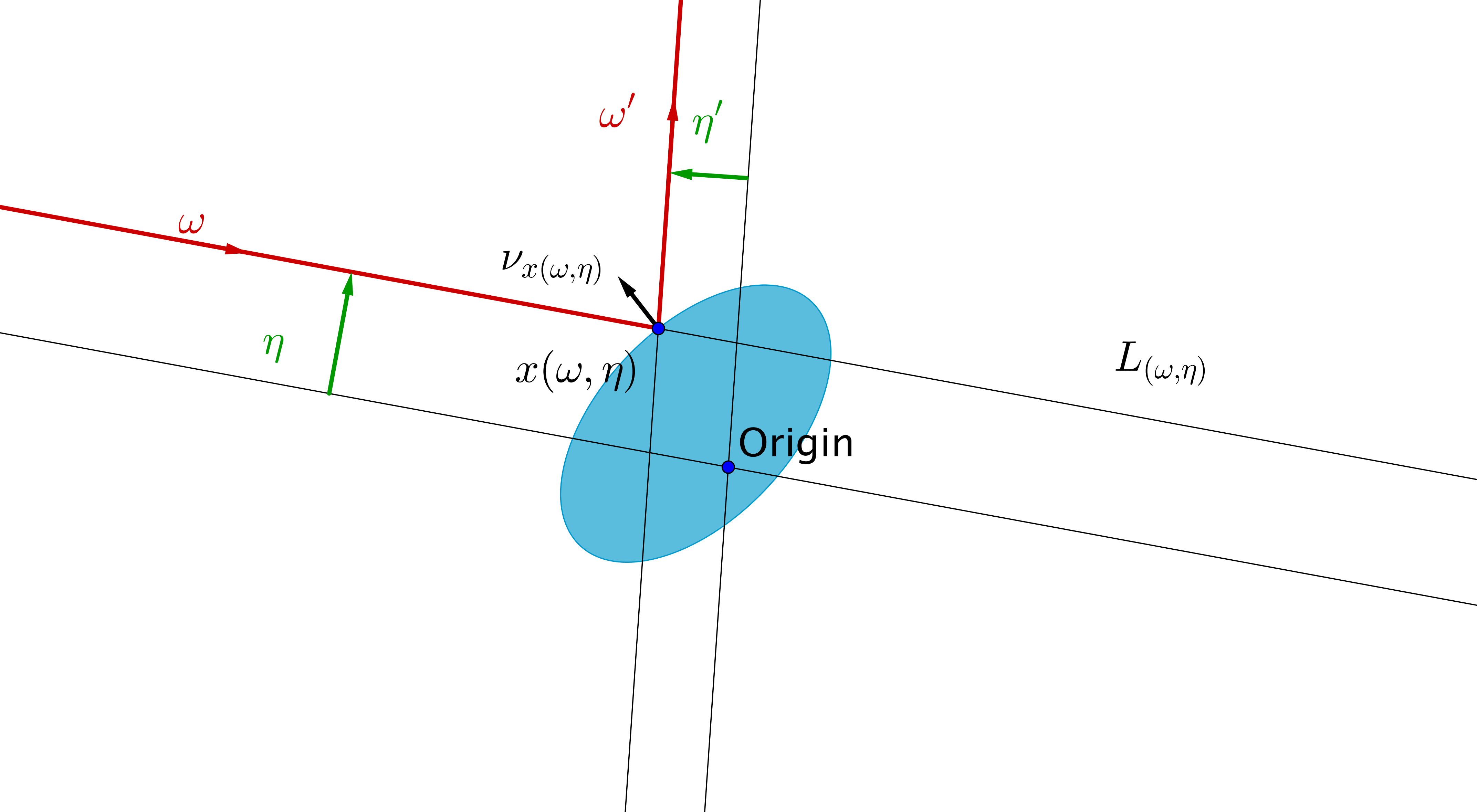 Figure 1
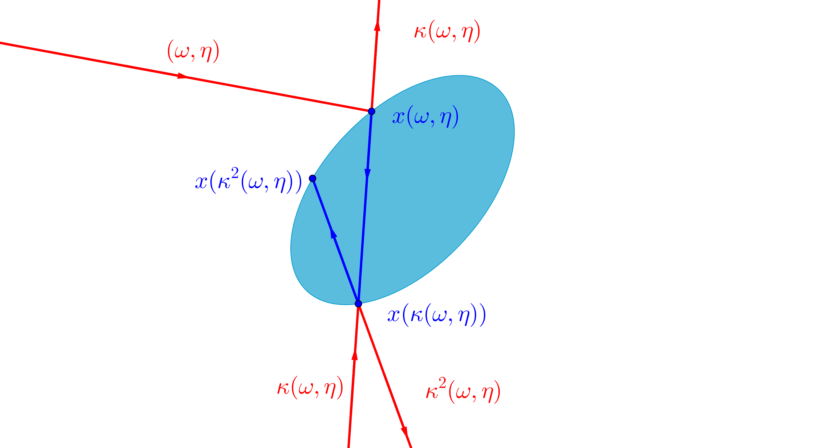 Figure 2
 Figure 3
 Figure 4
Peer Reviews
No public reviews on file for this paper yet. If you reviewed it on a platform where reviews are public (OpenReview, ICLR, NeurIPS, ICML), you can paste yours below so the community can read it here.
Videos
No videos yet. Explain this paper in a talk, walkthrough, or lecture? Add one.
Equidistribution of phase shifts in obstacle scattering
Jesse Gell-Redman
School of Mathematics and Statistics, University of Melbourne
and
Maxime Ingremeau
Institut de Recherche Mathématique Avancée, Université de Strasbourg
Abstract.
For scattering off a smooth, strictly convex obstacle with positive curvature, we show that the eigenvalues of the scattering matrix – the phase shifts – equidistribute on the unit circle as the frequency at a rate proportional to , under a standard condition on the set of closed orbits of the billiard map in the interior. Indeed, in any sector not containing , there are eigenvalues for large, where is a constant depending only on the dimension. Using this result, the two term asymptotic expansion for the counting function of Dirichlet eigenvalues, and a spectral-duality result of Eckmann-Pillet, we then give an alternative proof of the two term asymptotic of the total scattering phase due to Majda-Ralston [MR78].
1. Introduction
Let denote a strictly convex domain whose boundary is smooth and has positive sectional curvature. We shall write . It is well-known (see for instance [Mel95, §5] or [DZ, §4.4]) that for any and any , there is a unique solution to the Dirichlet problem
[TABLE]
such that
[TABLE]
where we write and . In particular is determined by and we define the scattering matrix , which depends on and , by
[TABLE]
extends to a unitary operator acting on with the property that is trace class [Tay11, RS79]. Therefore, for any , has purely discrete spectrum, accumulating only at 1, which we denote by . Our aim in this paper is to study the asymptotic distribution of the as .
Our main result is an estimate for the number of phase shifts in a sector as . Define the counting function
[TABLE]
where the eigenvalues are counted according to multiplicity. Letting where is the unit ball in , we will prove
[TABLE]
In particular, the phase shifts accumulate in each sector at a rate proportional to as times . The estimate in (1.2) follows from Theorem 1.1, see Section 5.
To study the asymptotic distribution of the phase shifts, consider the measure on the circle , defined for continuous functions by
[TABLE]
Note that is finite if . The following theorem describes the behavior as , provided (2.6) holds, which is a standard assumption on the volume of the periodic points of the inside billiard map. Note that this assumption holds if our smooth convex obstacle, is generic (see the discussion at the end of Section 2).
Theorem 1.1**.**
Let be a smooth strictly convex open set with positive sectional curvature, such that (2.6) holds. Then for any with , we have
[TABLE]
Remark 1.2**.**
The factor in front of the integral in (1.4) arises as the volume of the ‘interacting region’ in phase space of incoming rays from the sphere at infinity that make contact with the obstacle. See Section 2 for further description of the classical dynamics. In [GRHZ15], in which the first author and collaborators studied the same problem for semiclassical potential scattering, they defined a measure , depending on a semiclassical parameter , analogously to the measure in (1.3) except they included the volume of the interacting region. Here we prefer not to, so that the dependence on the interacting region appears explicitly in the limit measure.
As an application of the equidistribution of the measure , we will give an alternative proof of the following result of Majda-Ralston, generalized by Melrose and then by Robert, regarding the asymptotic development of the total scattering phase
[TABLE]
The scattering phase can be defined in a natural way so that .
Theorem 1.3** ([MR78, Mel88, Rob96]).**
Let be a smoothly bounded, strictly convex obstacle whose set of periodic billiard trajectories has measure zero. Then
[TABLE]
In fact, Theorem [Mel88, Rob96] holds for all smoothly bounded, compact domains satisfying the stated assumption on the periodic trajectories.
As we describe in Section 5, the novelty in our proof comes from its use of the explicit relationship between the counting function for the Dirichlet eigenvalues,
[TABLE]
and the scattering phase which arises from the spectral duality result of Eckmann-Pillet [EP95]. Indeed, note that the leading order term in (1.6) is times the leading order term in Weyl’s law [Ivr80], which is to be expected since, as explained in Section 5, ‘inside-outside’ duality says that a phase shift makes a complete rotation of the unit circle for each Dirichlet eigenvalue of .
Relation to other works
Since the pioneering works of Birman, Sobolev, and Yafaev (see for example [SY85, BY84]), there has been a wealth of literature on the asymptotic behavior of the scattering matrix at high energy, in particular about the distribution of phase shifts. In semi-classical potential scattering, an analogous result for compactly supported potentials was proven by the first author, Hassell, and Zelditch in [GRHZ15] for non-trapping potentials, and was generalized to trapping potentials by the second author in [Ing16a]. See [GRHZ15] for a complete literature review of phase shift asymptotics for potential scattering. The behaviour of the phase shifts in the semi-classical limit has been studied in various settings: for magnetic potentials ([BP12]), for scattering by radially symmetric potentials, in [DGRHH13], near resonant energies in [NP14]…
The idea of using trace formulae to analyze the asymptotics of the spectra comes from [Zel92, Zel97], and was the starting point of [GRHZ15], [Ing16a] and of the present paper. The main tool we use here is the Kirchhoff approximation, which was proven in its optimal form in [MT85]. Finally, our proof is simplified by describing the micro-local properties of the scattering matrix in terms of its action on Gaussian states, an approach which was introduced in [Ing16a] for potential scattering.
There do exist perturbations of the free Hamiltonian for which the phase shifts do not equidistribute. Indeed, for Schrödinger operators of the form where , , the first author and Hassell showed in [GRH15] that an appropriatly rescaled spectral measure for converges to the pushforward via the map of a homogeneous measure
[TABLE]
on , where and the are determied by . It would be interesting to know if there are circumstances under which equidistribution fails in the setting of obstacle scattering.
Organisation of the paper
In Section 2, we will recall a few facts about the classical scattering dynamics, and its links with the interior billiard dynamics. In Section 3, we will recall the main tools we use to prove Theorem 1.1. In Section 4, we prove Theorem 1.1 in the special case when is a polynomial vanishing at one. Finally, we prove Theorems 1.1 and 1.3 in Section 5. The appendix contain rather elementary facts of semiclassical analysis, and a proof of a resolution of identity formula on the sphere.
Acknowledgements
J.G.R. acknowledges the support of the Australian Research Council through Discovery Grant DP180100589. M.I. was funded by the LabEx IRMIA, and partially supported by the Agence Nationale de la Recherche project GeRaSic (ANR-13-BS01-0007-01). Both authors wish to thank the Australian Mathematical Sciences Institute and the Mathematical Sciences Institute at the Australian National University for their partial funding of the workshop “Microlocal Analysis and its Applications in Spectral Theory, Dynamical Systems, Inverse Problems, and PDE” at which part this project was completed.
2. Classical scattering dynamics and interior dynamics
Let and . We will always identify with a point in . Consider the line . By strict convexity of , it intersects in zero, one or two points. We define the interaction region,
[TABLE]
If , then there exists such that . We then set (see Figure 1)
[TABLE]
where is the outward pointing normal vector at the point . We then set
[TABLE]
If , we shall set . The map may then be seen as a map , which is smooth (and even symplectic) away from the glancing set .
Using Cauchy’s surface area formula, it is straightforward that
[TABLE]
For , we will denote by the set of fixed points of . Note that we then have
[TABLE]
and that is exactly the ‘glancing set’, i.e. the set of such that consists of a single point. We define
[TABLE]
the set of non-trivial glancing periodic points with period , also an invariant subset.
The sets will play a central role in our proof, and can be better understood in terms of the periodic points of the interior billiard map, as follows. Consider the set . If , there will be a unique such that . We shall then write , and . We have , and we may define by . The map , and we shall denote by the set of periodic points of period of .
The following elementary lemma makes explicit the link between and , as can be seen on Figure 2.
Lemma 2.1**.**
Let . We then have
[TABLE]
As a consequence of this lemma, we see that is homeomorphic to .
The volume of the set of fixed points
Let us denote by the (symplectic) volume on . We will always assume that we have
[TABLE]
This condition may of course be rephrased in terms of the dynamics of on . If is any Riemannian volume and is any Riemannian distance on the manifold , Equation (2.5) is equivalent to
[TABLE]
Condition (2.6) is conjectured to hold for all domains , not necessarily convex. This conjecture, known as Ivrii’s conjecture, has implications in terms of remainders for the Weyl’s law for the eigenvalues of the Laplacian (see [Ivr80]). In the generic case, it was shown in [PS88] that is finite for all , so that (2.6) holds. If the manifold is analytic, then the map will be analytic, and we can show that (2.6) will hold (see for instance [SV97]).
3. Tools for the proof of Proposition 4.1
Before proving Proposition 4.1, let us recall a few facts we will need in the proof.
3.1. An integral representation for the scattering amplitude
The operator
[TABLE]
can also be defined as follows. Let be the unique solutions to
[TABLE]
satisfying the Sommerfeld radiation condition.
may then be written as
[TABLE]
One can show (see for instance [HR76], page 381) that is given by an integral kernel
[TABLE]
where satisfies
[TABLE]
3.2. The Kirchhoff approximation
The function was studied in [MT85], where the authors write
[TABLE]
The main result we need from them can be summed up as follows. (The definition of the symbol classes is recalled in Appendix A.)
Theorem 3.1** (Melrose-Taylor, [MT85]).**
[TABLE]
where is the outward pointing normal vector at the point , and where satisfies
[TABLE]
In particular, we have
[TABLE]
We therefore have
[TABLE]
3.3. The use of Gaussian states
From now on, we fix a smooth compactly supported function
[TABLE]
taking value in a neighborhood of [math]. Let . We set
[TABLE]
Note that . The term \chi\big{(}k^{1/4}|\omega-\omega_{0}|\big{)} is not very important here, and we could replace it by \chi\big{(}k^{p}|\omega-\omega_{0}|\big{)} for any . It is here only to ensure that the integrals in (3.10) and (3.11) below makes sense.
The following lemma, whose proof can be found in [Ing16b, §4], says that any function can be decomposed along the through a resolution of identity formula.
Lemma 3.2**.**
1) Let . We have
[TABLE]
where is a parameter depending on , with
[TABLE]
2) Let a trace class operator, then
[TABLE]
Let be some Riemannian distance on . For any , the set
[TABLE]
has volume . Therefore, since , we have
[TABLE]
3.4. The action of the scattering matrix on a Gaussian state
The main tool we use in the proof of Theorem 1.1 is the following proposition, which describes the action of the scattering matrix on a Gaussian state
Proposition 3.3**.**
Let . Let us write . We have
[TABLE]
where
[TABLE]
* has a non-negative imaginary part vanishing only at , and , and has a positive definite imaginary part.*
Proof.
Thanks to (3.9, we have
[TABLE]
This is an oscillatory integral with a phase
[TABLE]
Let be the points such that and . Let be such that and . We also set . Note that
[TABLE]
The phase has a vanishing gradient and imaginary part at four points: , , and .
We will show below that the second derivative of is non-degenerate at these critical points. In particular, this implies thanks to Lemma A.1 that \big{(}(S_{k}-Id)\phi_{\omega_{0},\eta_{0}}\big{)}(\theta)=O(k^{-\infty}), unless, for some , we have .
We shall write
[TABLE]
so that , and .
Let us take a partition of unity on :
[TABLE]
with , satisfying in a neighborhood of . We shall consider the two integrals
[TABLE]
To analyse these integrals, let us introduce more convenient local coordinates.
Local Coordinates
We shall write the points close to as
[TABLE]
where , , . Here, is the second fundamental form of at , and is therefore a positive definite symmetric matrix.
Similarly, we shall write the points close to as
[TABLE]
where , , .
Finally, for , we shall write the points close to , as
[TABLE]
where , , .
In these coordinates, using the fact that , we have
[TABLE]
Since we are working away from the glancing set, the space is of dimension . By definition of , we have
[TABLE]
for . Starting from an orthonormal basis of , we may find an orthonormal basis of , an orthonormal basis of and an orthonormal basis of such that, if , and are written in the coordinates associated to these bases, we have
[TABLE]
where, notation as in (3.19),
[TABLE]
and where we denote by the canonical scalar product on .
We therefore have
[TABLE]
where
[TABLE]
We may then write
[TABLE]
where comes from the Jacobian of the change of coordinates , and satisfies .
3.4.1. Behavior for close to
The matrix is invertible, with inverse
[TABLE]
and we have, notation as in (3.19),
[TABLE]
For close to , is still invertible, with inverse
[TABLE]
By applying Lemma A.2, we obtain that
[TABLE]
Recall that we assume in this paragraph that |\theta-\theta_{0}|=O_{\varepsilon}\big{(}k^{-1/2+\varepsilon}\big{)} for all . Noting that , we deduce that
[TABLE]
Therefore, we have for all close to .
[TABLE]
3.4.2. Behavior for close to
Note that the matrix
[TABLE]
is invertible, since the second term is real symmetric, so that it does not have in its spectrum. It is then straightforward to check that is invertible, with inverse
[TABLE]
Applying Lemma A.2, we obtain that for , we have
[TABLE]
where
[TABLE]
Therefore, we have
[TABLE]
We therefore have
[TABLE]
where
[TABLE]
and satisfies the announced properties, thanks to (3.18). ∎
4. Proof of Theorem 1.1
The main ingredient in the proof of Theorem 1.1 is a trace formula for powers of :
Proposition 4.1**.**
Suppose that (2.6) holds. Let . We have
[TABLE]
In particular, for any trigonometric polynomial vanishing at and for the measure in (1.3), as ,
[TABLE]
Theorem 1.1 can be deduced from Proposition 4.1 in exactly the same way as in [Ing16a, §5]. We refer the reader to this paper for the argument.
Before proving Proposition 4.1, we shall prove the following corollary of Proposition 3.3.
Corollary 4.2**.**
Let , let . Let us write . We have
[TABLE]
where for all ,
[TABLE]
and is such that we have
[TABLE]
for all satisfying for some .
Proof.
We shall prove this result by induction. For , the result is an immediate corollary of Proposition 3.3 and of the non-stationary phase Lemma A.1. Suppose that we have proven the result for some , and let us prove it for . By assumption, we have
By Lemma 3.2, we have
[TABLE]
where is equivalent to some power of .
We therefore have
[TABLE]
We shall write
[TABLE]
In , the term is small in norm by recurrence hypothesis, since is unitary. For the other term, we note that the term in the integrand is as soon as is at a distance larger than from . Hence, the integrand is away from a set of volume for some . On this set, the integrand has an norm bounded by . Therefore, .
As for , we have
[TABLE]
Now, by the induction hypothesis, we know that the above integrand is unless \mathrm{d}(\kappa(\omega^{\prime},\eta^{\prime}),(\omega_{p},\eta_{p}))=O\big{(}k^{-1/2+\varepsilon}\big{)} and \mathrm{d}((\omega,\eta),(\omega^{\prime},\eta^{\prime}))=O\big{(}k^{-1/2+\varepsilon}\big{)}. The result follows. ∎
We are now ready to prove Proposition 4.1.
Proof of Proposition 4.1.
First of all, let us note that it is enough to show the result for . Indeed, since is unitary, we have
[TABLE]
Therefore, let us fix from now on . By (3.11), we have
[TABLE]
By (3.13), the second term in the right-hand side of (4.2) is
To deal with the first term, we note that, when computing \big{(}S_{k}-Id\big{)}\phi_{\omega_{0},\eta_{0}}(\theta), the phase satisfies . Therefore, Lemma A.1 implies that we have
[TABLE]
Therefore, the first term in the right-hand side of (4.2) is
We now compute
[TABLE]
Now, by Corollary 4.2, the integrand is as soon as . But, by (2.6), the volume of the set of satisfying is a . All in all, we obtain that
[TABLE]
Therefore, (4.2) gives us
[TABLE]
and the result follows since this is true for all . ∎
5. Proof of theorem 1.3
We now give our alternative proof of the scattering phase asymptotics in Theorem 1.3. We begin by recalling that the scattering phase can be defined continuously in such a way that and thus defined is in fact smooth for all . We define the ‘reduced’ scattering phase by the sum
[TABLE]
where the logarithms of the eigenvalues, the are chosen to take values in . For fixed the eigenvalues accumulate at from the bottom half plane and thus contribute positive values to the sum, which is nonetheless finite. A result of Eckmann-Pillet [EP95] shows that eigenvalues approach with positive imaginary part if and only if approaches a Dirichlet eigenvalue of . In fact, with as in (1.7), we have
[TABLE]
Under the hypothesis that the measure of the periodic billiard trajectories in is zero, it is known [Ivr80] that
[TABLE]
We claim that
[TABLE]
We will prove this by breaking up the unit circle into sectors of size estimating the sum defining in these sectors. Namely, let and , so that
[TABLE]
We begin with , which is distinct from since there are infinitely many phase shifts in . We are going to show that
[TABLE]
Thanks to equation (2.3) in [Chr15] (which relies on the methods developed in [Zwo89]), we have that there exists independent of and such that
[TABLE]
Let us write
[TABLE]
Using (5.1) and a constant whose value changes from line to line, we see that
[TABLE]
For , we estimate from above and below, and clearly
[TABLE]
It follows from the (1.2), since our sectors are size , that for , for any and , there is a constant such that
[TABLE]
Since we have
[TABLE]
and thus
[TABLE]
for any . Taking and sending gives the result.
Appendix A Symbol classes and stationary phase
Let be a compact manifold, and let be a family of -valued functions in , and let . We shall write that if
[TABLE]
The following lemma follows from [Hör83, Lemma 7.7.1].
Lemma A.1**.**
Let . Let , and . Suppose that there exists such that for all in the support of , we have . We then have
[TABLE]
The following stationary phase result is a variant over [Hör83, Theorem 7.7.5], but we recall its proof for completeness. Note that we do not assume that the derivative of the phase vanishes at the origin, but only that for all .
Lemma A.2**.**
Let have a positive imaginary part, and be such that
- •
There exists such that for all , .
- •
* is invertible for every , and there exists independent of such that*
[TABLE]
Let . Let us write . We have
[TABLE]
where the square-root of the determinant is defined as in [Hör83, §3.4].
In particular, if , we have , so that we have
[TABLE]
Proof.
Let be such that if , and . Set . We may write
[TABLE]
By Lemma A.1 and the assumption we made on , the second integral is .
We have
[TABLE]
and
[TABLE]
Indeed, all the derivatives of will vanish for such , and, when differentiating e^{ik\big{(}\varphi_{k}(x)-\varphi_{k}(0)-x\cdot\partial\varphi_{k}(0)-\frac{1}{2}x\cdot\partial^{2}\varphi_{k}(0)x\big{)}} once, we get a factor of size . Differentiating again, each derivation makes the function grow at most of a factor .
Let us write b_{k}(x):=a_{k}(x)\chi_{k}(x)e^{ik\big{(}\varphi_{k}(x)-\varphi_{k}(0)-x\cdot\partial\varphi_{k}(0)-\frac{1}{2}x\cdot\partial^{2}\varphi_{k}(0)x\big{)}}, so that . We have
[TABLE]
Let us write , and . We have
[TABLE]
so that, setting , we have
[TABLE]
Writing and , we therefore have
[TABLE]
Now, we have
[TABLE]
so that by Plancherel’s equality,
[TABLE]
Thanks to [Hör83, Theorem 7.6.5], this quantity is equal to
[TABLE]
Since and , the remainder can be made smaller than any power of by taking large enough.
Using (A.2), we see that there exists such that
[TABLE]
The first term in the sum is , and the following ones are . The statement follows. ∎
The reference list from the paper itself. Each links out to its DOI / PubMed record.
- 1[BP 12] Daniel Bulger and Alexander Pushnitski. The spectral density of the scattering matrix for high energies. Comm. Math. Phys. , 316(3):693–704, 2012.
- 2[BY 84] M. Sh. Birman and D. R. Yafaev. Asymptotic behaviour of the spectrum of the scattering matrix. J. Sov. Math. , 25:793–814, 1984.
- 3[Chr 15] T.J. Christiansen. A sharp lower bound for a resonance-counting function in even dimensions. ar Xiv preprint ar Xiv:1510.04952 , 2015.
- 4[DGRHH 13] K. Datchev, J. Gell-Redman, A. Hassell, and P. Humphries. Approximation and equidistribution of phase shifts: spherical symmetry. to appear in Comm. Math. Phys. , 2013.
- 5[DZ] Semyon Dyatlov and Maciej Zworski. Mathematical theory of scattering resonances, book in preparation.
- 6[EP 95] Jean-Pierre Eckmann and Claude-Alain Pillet. Spectral duality for planar billiards. Comm. Math. Phys. , 170(2):283–313, 1995.
- 7[GRH 15] Jesse Gell-Redman and Andrew Hassell. The distribution of phase shifts for semiclassical potentials with polynomial decay. ar Xiv:1509.03468 , 2015.
- 8[GRHZ 15] Jesse Gell-Redman, Andrew Hassell, and Steve Zelditch. Equidistribution of phase shifts in semiclassical potential scattering. J. Lond. Math. Soc. (2) , 91(1):159–179, 2015.