The properties of the first galaxies in the BLUETIDES simulation
Stephen M. Wilkins, Yu Feng, Tiziana Di-Matteo, Rupert Croft,, Christopher C. Lovell, Dacen Waters

TL;DR
This study uses the BLUETIDES simulation to predict properties of early galaxies during reionisation, matching observational data and revealing insights into star formation, dust attenuation, and black hole activity at high redshift.
Contribution
First large-scale hydrodynamical simulation to predict detailed properties of galaxies during reionisation, aligning with observations and exploring black hole contributions.
Findings
Galaxy population matches observed stellar mass and UV luminosity functions.
Star formation rates increase rapidly and are largely independent of stellar mass.
Active SMBHs contribute around 3% to galaxy UV luminosities on average.
Abstract
We employ the very large cosmological hydrodynamical simulation BLUETIDES to investigate the predicted properties of the galaxy population during the epoch of reionisation (). BLUETIDES has a resolution and volume () providing a population of galaxies which is well matched to depth and area of current observational surveys targeting the high-redshift Universe. At BLUETIDES includes almost 160,000 galaxies with stellar masses . The population of galaxies predicted by BLUETIDES closely matches observational constraints on both the galaxy stellar mass function and far-UV () luminosity function. Galaxies in BLUETIDES are characterised by rapidly increasing star formation histories. Specific star formation rates decrease with redshift though remain largely insensitive to stellar mass. As a result of the…
Click any figure to enlarge with its caption.
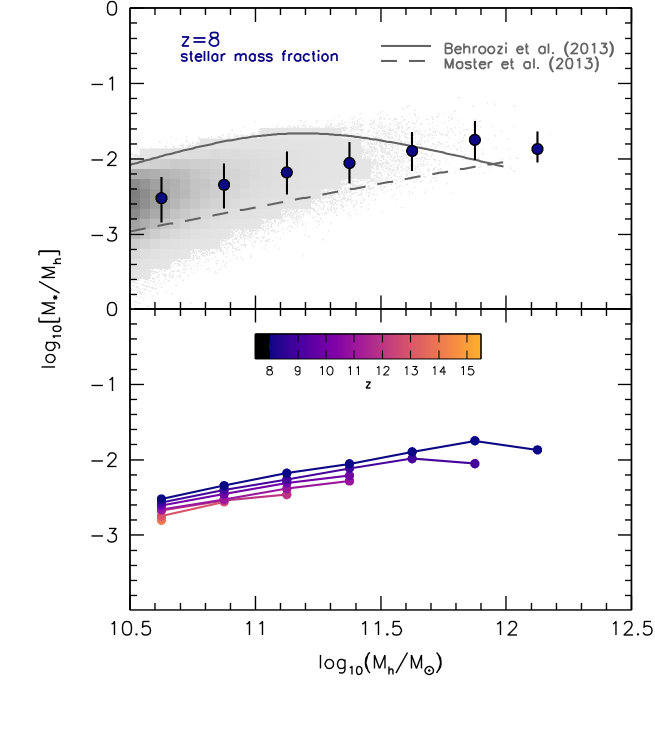 Figure 1
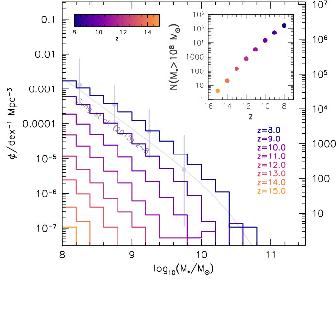 Figure 2
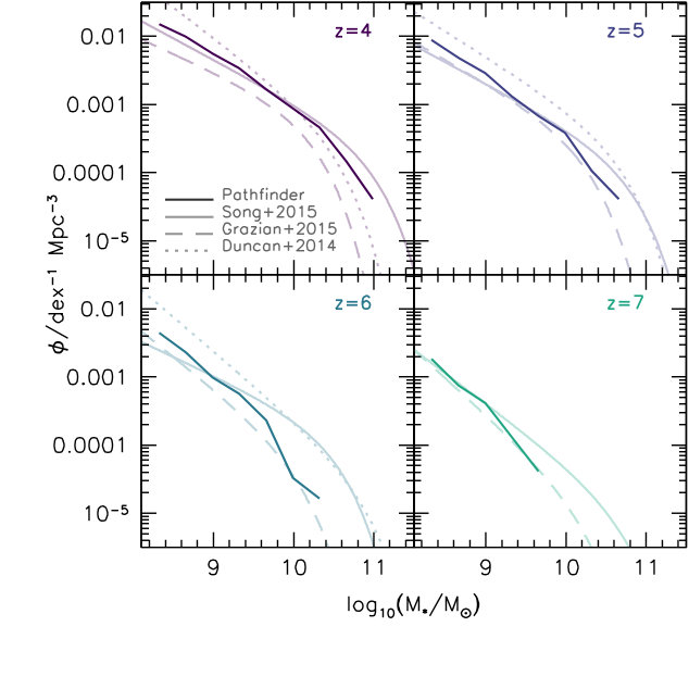 Figure 3
 Figure 4
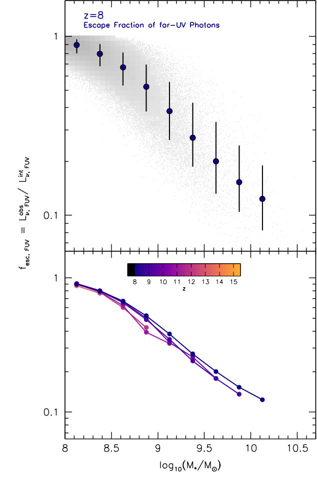 Figure 5
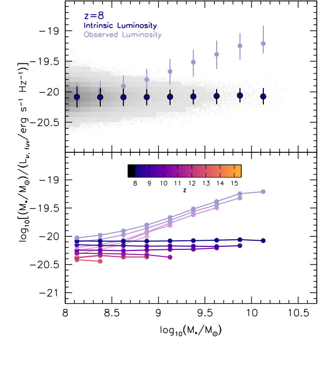 Figure 6
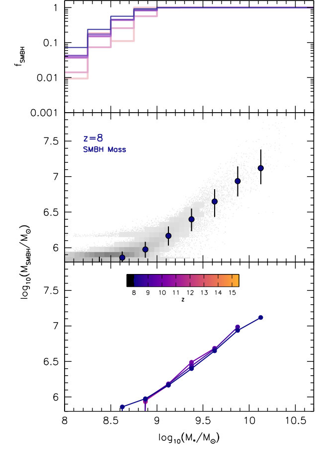 Figure 7
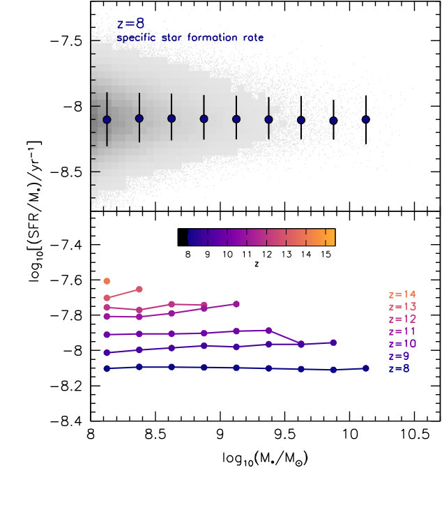 Figure 8
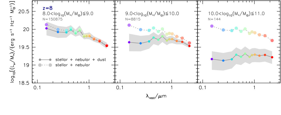 Figure 9
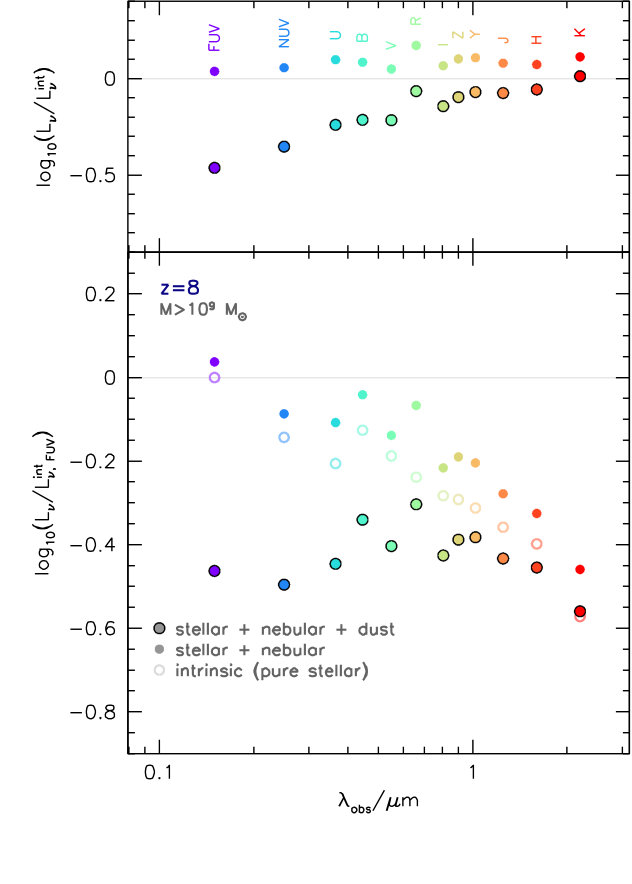 Figure 10
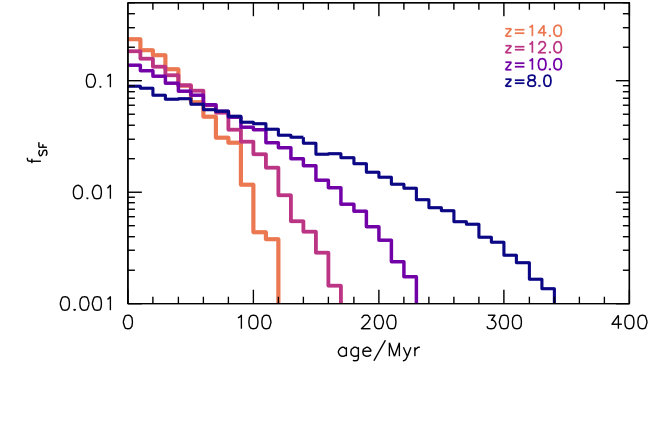 Figure 11
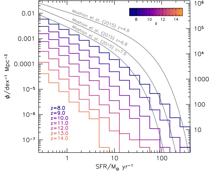 Figure 12
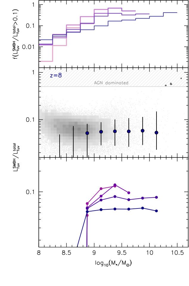 Figure 13
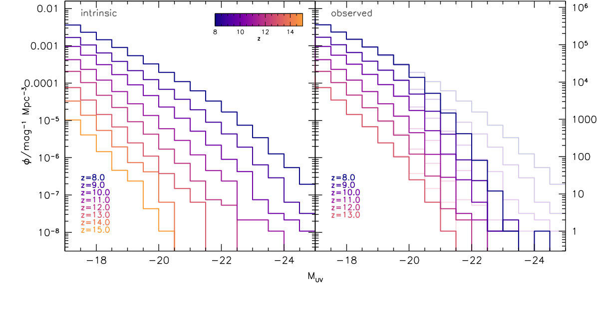 Figure 14
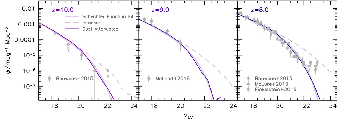 Figure 15
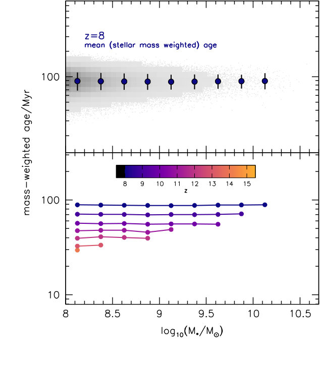 Figure 16
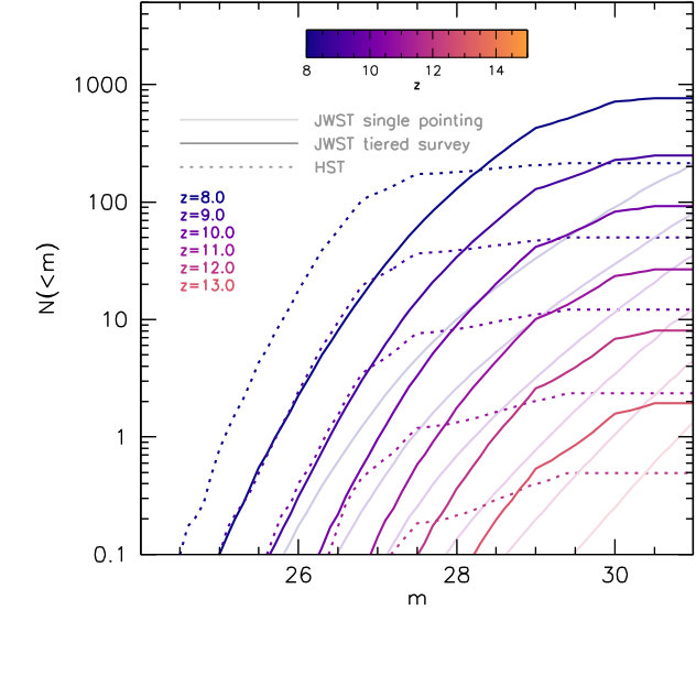 Figure 17
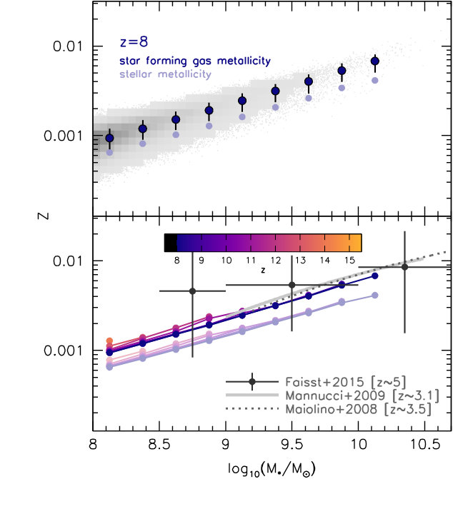 Figure 18
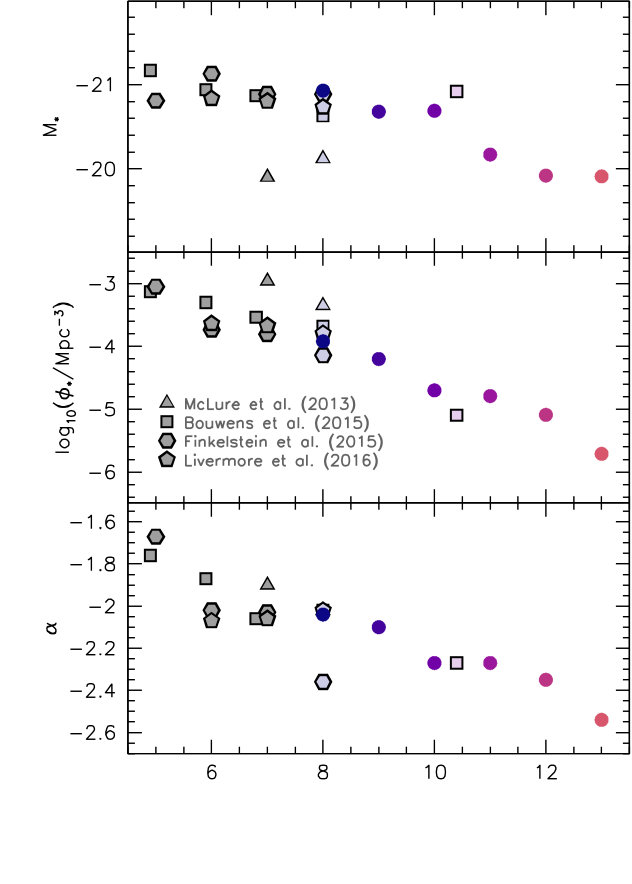 Figure 19
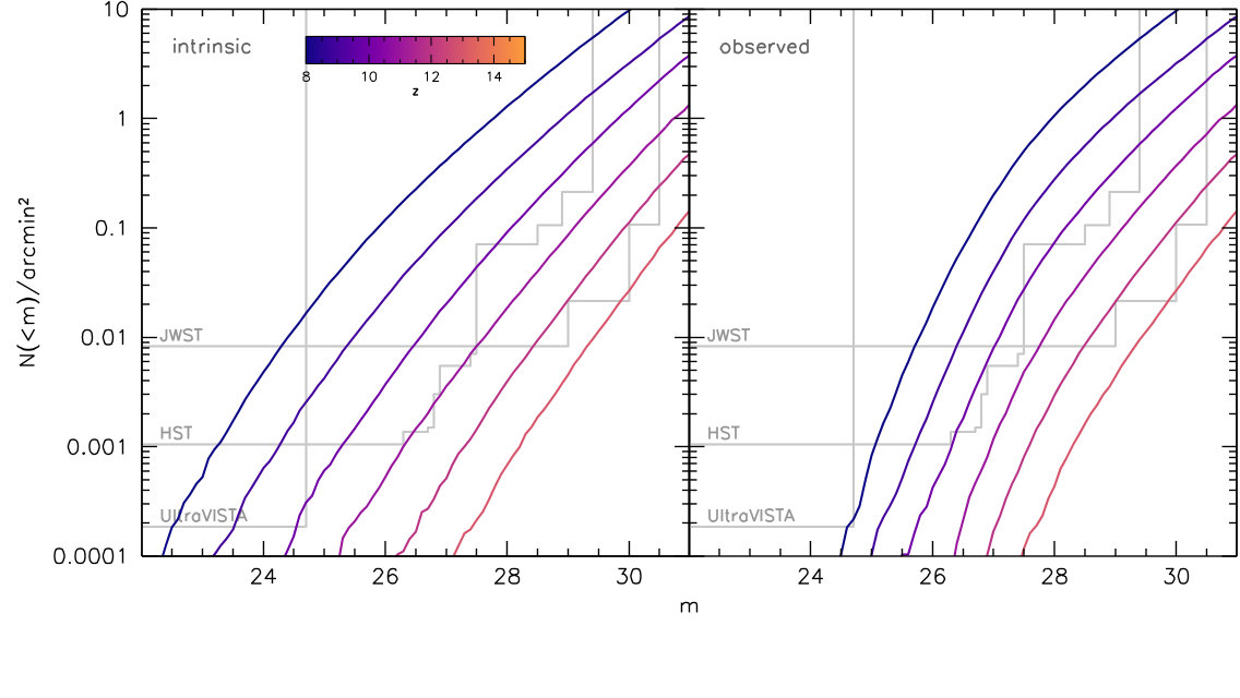 Figure 20
| 13 | -19.91 | -5.71 | -2.54 |
|---|---|---|---|
| 12 | -19.92 | -5.09 | -2.35 |
| 11 | -20.17 | -4.79 | -2.27 |
| 10 | -20.69 | -4.70 | -2.27 |
| 9 | -20.68 | -4.20 | -2.10 |
| 8 | -20.93 | -3.92 | -2.04 |
| - | - | - | - | - | - | - | |
| stellar-to-dark matter mass ratio - | |||||||
| 13.0 | - | - | - | - | - | ||
| 12.0 | - | - | - | - | |||
| 11.0 | - | - | - | ||||
| 10.0 | - | - | - | ||||
| 9.0 | - | ||||||
| 8.0 | |||||||
| - | ||||||
| - | ||||||
| - | ||||||
| - | - | |||||
| - | - | |||||
| - | - | - | ||||
| - | - | - | - | |||
| - | - | - | - | |||
| - | - | - | - | - | ||
| - | - | - | - | - | ||
| - | - | - | - | - | - | |
| - | - | - | - | - | - | |
| - | ||||||
| - | ||||||
| - | ||||||
| - | ||||||
| - | ||||||
| - | ||||||
| - | ||||||
| - | ||||||
| - | - | |||||
| - | - | - | ||||
| - | - | - | ||||
| - | - | - | - | |||
| - | - | - | - | - | ||
| - | - | - | - | - | ||
| - | - | - | - | - | - | |
| - | - | - | - | - | - | |
| - | - | - | - | - | - | - | - | - | |
| median specific star formation rate - | |||||||||
| 13.0 | - | - | - | - | - | - | - | ||
| 12.0 | - | - | - | - | - | ||||
| 11.0 | - | - | - | - | |||||
| 10.0 | - | - | |||||||
| 9.0 | - | ||||||||
| 8.0 | |||||||||
| median mass-weighted age - | |||||||||
| 13.0 | 33 | 33 | - | - | - | - | - | - | - |
| 12.0 | 39 | 41 | 40 | 40 | - | - | - | - | - |
| 11.0 | 47 | 48 | 48 | 46 | 49 | - | - | - | - |
| 10.0 | 57 | 56 | 56 | 56 | 56 | 56 | 56 | - | - |
| 9.0 | 71 | 71 | 70 | 70 | 70 | 70 | 70 | 71 | - |
| 8.0 | 89 | 88 | 88 | 88 | 87 | 88 | 88 | 89 | 89 |
| median star forming gas metallicity - | |||||||||
| 13.0 | - | - | - | - | - | - | - | ||
| 12.0 | - | - | - | - | - | ||||
| 11.0 | - | - | - | - | |||||
| 10.0 | - | - | |||||||
| 9.0 | - | ||||||||
| 8.0 | |||||||||
| median stellar metallicity - | |||||||||
| 13.0 | - | - | - | - | - | - | - | ||
| 12.0 | - | - | - | - | - | ||||
| 11.0 | - | - | - | - | |||||
| 10.0 | - | - | |||||||
| 9.0 | - | ||||||||
| 8.0 | |||||||||
| - | - | - | - | - | - | - | - | - | |
| median far-UV photon escape fraction | |||||||||
| 13.0 | 0.87 | 0.77 | - | - | - | - | - | - | - |
| 12.0 | 0.91 | 0.78 | 0.6 | 0.43 | - | - | - | - | - |
| 11.0 | 0.9 | 0.79 | 0.62 | 0.39 | 0.32 | - | - | - | - |
| 10.0 | 0.91 | 0.8 | 0.67 | 0.5 | 0.33 | 0.26 | 0.18 | - | - |
| 9.0 | 0.9 | 0.8 | 0.65 | 0.49 | 0.35 | 0.24 | 0.18 | 0.14 | - |
| 8.0 | 0.89 | 0.8 | 0.67 | 0.52 | 0.38 | 0.27 | 0.2 | 0.15 | 0.12 |
| - | - | - | - | - | - | - | - | - | |
| median intrinsic mass-to-light ratio - | |||||||||
| 13.0 | - | - | - | - | - | - | - | ||
| 12.0 | - | - | - | - | - | ||||
| 11.0 | - | - | - | - | |||||
| 10.0 | - | - | |||||||
| 9.0 | - | ||||||||
| 8.0 | |||||||||
| median observed mass-to-light ratio - | |||||||||
| 13.0 | - | - | - | - | - | - | - | ||
| 12.0 | - | - | - | - | - | ||||
| 11.0 | - | - | - | - | |||||
| 10.0 | - | - | |||||||
| 9.0 | - | ||||||||
| 8.0 | |||||||||
| intrinsic far-UV luminosity function | ||||||
| - | - | - | - | - | - | |
| - | - | - | - | - | - | |
| - | - | - | - | - | ||
| - | - | - | - | - | ||
| - | - | - | - | |||
| - | - | - | ||||
| - | - | - | ||||
| - | - | |||||
| - | ||||||
| - | ||||||
| - | ||||||
| - | ||||||
| - | ||||||
| - | ||||||
| - | ||||||
| - | ||||||
| observed (dust-corrected) far-UV luminosity function | ||||||
| - | - | - | - | - | - | |
| - | - | - | - | - | ||
| - | - | - | - | |||
| - | - | - | ||||
| - | - | |||||
| - | ||||||
| - | ||||||
| - | ||||||
| - | ||||||
| - | ||||||
| - | ||||||
| - | ||||||
| - | - | - | - | - | - | - | - | - | |
| median SMBH mass - | |||||||||
| 13.0 | - | - | - | - | - | - | - | - | - |
| 12.0 | - | - | - | 5.93 | - | - | - | - | - |
| 11.0 | - | - | - | 5.95 | 6.17 | - | - | - | - |
| 10.0 | - | - | - | 5.96 | 6.19 | 6.49 | 6.69 | - | - |
| 9.0 | - | - | - | 5.97 | 6.18 | 6.44 | 6.68 | 6.99 | - |
| 8.0 | - | - | 5.86 | 5.98 | 6.17 | 6.4 | 6.65 | 6.94 | 7.12 |
Peer Reviews
No public reviews on file for this paper yet. If you reviewed it on a platform where reviews are public (OpenReview, ICLR, NeurIPS, ICML), you can paste yours below so the community can read it here.
Videos
No videos yet. Explain this paper in a talk, walkthrough, or lecture? Add one.
The properties of the first galaxies in the BlueTides simulation
Stephen M. Wilkins,1 Yu Feng,2,3 Tiziana Di-Matteo,2 Rupert Croft,2Christopher C. Lovell,1 Dacen Waters2,
1 Astronomy Centre, Department of Physics and Astronomy, University of Sussex, Brighton, BN1 9QH, UK
2 McWilliams Center for Cosmology, Carnegie Mellon University, Pittsburgh PA, 15213, USA
3 Berkeley Center for Cosmological Physics, University of California, Berkeley, Berkeley CA, 94720, USA E-mail: [email protected]
(Accepted XXX. Received YYY; in original form ZZZ)
Abstract
We employ the very large cosmological hydrodynamical simulation BlueTides to investigate the predicted properties of the galaxy population during the epoch of reionisation (). BlueTides has a resolution and volume () providing a population of galaxies which is well matched to depth and area of current observational surveys targeting the high-redshift Universe. At BlueTides includes almost 160,000 galaxies with stellar masses . The population of galaxies predicted by BlueTides closely matches observational constraints on both the galaxy stellar mass function and far-UV () luminosity function. Galaxies in BlueTides are characterised by rapidly increasing star formation histories. Specific star formation rates decrease with redshift though remain largely insensitive to stellar mass. As a result of the enhanced surface density of metals more massive galaxies are predicted to have higher dust attenuation resulting in a significant steepening of the observed far-UV luminosity function at high luminosities. The contribution of active SMBHs to the UV luminosities of galaxies with stellar masses is around on average. Approximately of galaxies with are predicted to have active SMBH which contribute of the total UV luminosity.
keywords:
galaxies: high-redshift – galaxies: photometry – methods: numerical – galaxies: luminosity function, mass function
††pubyear: 2015††pagerange: The properties of the first galaxies in the BlueTides simulation–LABEL:lastpage
1 Introduction
Within the first few hundred million years after the big bang the first stars and galaxies began to form, subsequently bringing an end to the cosmological dark ages. These early galaxies likely produced the ionising photons (either through star formation or from accretion on to super-massive black holes) responsible for the reionisation of hydrogen (e.g. Wilkins et al., 2011; Bouwens et al., 2012; Robertson et al., 2013; Robertson et al., 2015; Bouwens et al., 2015b).
This critical period of the Universe’s history is now observationally accesible thanks largely to the Hubble Space Telescope. Large samples of star forming galaxies have now been identified at and beyond (e.g. Bouwens et al., 2011, 2012, 2015a; Oesch et al., 2010, 2012b; Bunker et al., 2010; Wilkins et al., 2010; Wilkins et al., 2011; Finkelstein et al., 2010, 2012, 2015; Lorenzoni et al., 2011, 2013; McLure et al., 2011, 2013; Ellis et al., 2013; Laporte et al., 2014, 2015, 2016; Schmidt et al., 2014; Atek et al., 2015a, b).
Recently, the first small samples have been identified at (e.g. Oesch et al., 2012a, 2013, 2014, 2015, 2016; Ellis et al., 2013; McLeod et al., 2015; McLeod et al., 2016), approximately after the big bang. By taking advantage of gravitational lensing (e.g. Atek et al., 2015a, b) and wider-area ground based surveys (e.g. Bowler et al., 2014, 2015) galaxies have now been observed at with luminosities spanning a range of four orders of magnitude. The large samples now assembled allow constraints to be placed on the observed UV luminosity function, the star formation rate distribution function (e.g. Smit et al., 2012), and the galaxy stellar mass function (e.g. Grazian et al., 2015; Song et al., 2015).
In the near future, the James Webb Space Telescope (JWST) will revolutionise the study of the early phase of galaxy formation. JWST will provide sensitive near/mid-IR imaging and spectroscopy with high-spatial resolution. This will potentially allow the discovery of star forming galaxies to and allow the characterisation of the rest-frame UV-optical spectral energy distributions of high-redshift galaxies, providing both accurate redshifts and the robust determination of physical properties (e.g. gas phase metallicities, and star formation rates) through optical emission lines. JWST will be complemented by the Atacama Large Millimetre Array (ALMA) which will provide constraints on rest-frame far-IR emission of galaxies at high-redshift (e.g. Watson et al., 2015). In the longer term the Wide Field Infrared Survey Telescope (WFIRST) is expected (Waters et al., 2016a) to identify large numbers of galaxies to while the upcoming generation of extremely large telescopes will provide much greater spatial and spectral resolution allowing the detailed study of galaxies at very-high redshift.
Through comparisons with predictions from galaxy formation models the observations obtained by Hubble, and in the future JWST and WFIRST, will provide the opportunity to test and refine the physics of structure formation, reionisation, and early galaxy formation and evolution. Galaxy formation models can also be used to test and refine observational techniques, for example by assessing how accurately and precisely various physical properties can be recovered (e.g. Pforr et al., 2012, 2013; Smith & Hayward, 2015) and to influence observational survey strategy; this is particularly important at high-redshift where there are limited existing observations.
As part of an effort to understand the evolution of galaxies in the Universe and specifically make predictions for both JWST and WFIRST (Waters et al., 2016a) we have carried out a new simulation, BlueTides (Feng et al., 2015, 2016). BlueTides builds upon our previous simulations MassiveBlack-I (Di Matteo et al., 2012) and MassiveBlack-II (Khandai et al., 2015; Wilkins et al., 2013) and reaches an unprecedented combination of volume and resolution evolving a cube to with particles. BlueTides has a resolution comparable to Illustris (Vogelsberger et al., 2014) and Eagle (Schaye et al., 2015) but simulates a much larger (approximately larger) volume.
BlueTides also builds upon and complements previous efforts to specifically simulate and model the high-redshift Universe. Recent studies include results from both semi-analytical modelling (e.g. Clay et al., 2015; Angel et al., 2016; Mutch et al., 2016a; Liu et al., 2016; Geil et al., 2016; Mutch et al., 2016b; Liu et al., 2017; Cowley et al., 2017) and fully hydrodynamical simulations (e.g. Finlator et al., 2006, 2011; Jaacks et al., 2012; Di Matteo et al., 2012; Johnson et al., 2013; Paardekooper et al., 2013; Dayal et al., 2013; Agarwal et al., 2014; Davis et al., 2014; Shimizu et al., 2014; Khandai et al., 2015; Feng et al., 2015; Elliott et al., 2015; Paardekooper et al., 2015; Yajima et al., 2015; Feng et al., 2016; Jaacks et al., 2016; Shimizu et al., 2016; Finlator et al., 2017; Pawlik et al., 2017; Cullen et al., 2017).
In this study we explore the physical and photometric properties of the galaxy population predicted by BlueTides. We begin, in Section 2, by describing the BlueTides simulation. We then, in Section 3, focus on the predicted physical properties of the galaxy population. These include the galaxy stellar mass function (§3.2), star formation histories (§3.4), and metal enrichment (§3.5). In Section 4 we present predictions for some of the photometric properties of galaxies, including dust attenuation (§4.1.2), average spectral energy distributions (§4.2), and the far-UV luminosity function (§4.3). Section 5 presents predictions for the masses of super-massive black holes and their contribution to the far-UV luminosities of galaxies (§5.1). Finally, in Section 6, we present our conclusions. In Appendix A, we present tables containing the information used to create most of the figures presented in this paper.
2 The BlueTides Simulation
The BlueTides simulation (http://bluetides-project.org/, see Feng et al., 2015, 2016, for description of the simulation physics) was carried out using the Smoothed Particle Hydrodynamics code MP-Gadget with particles using the Blue Waters system at the National Centre for Supercomputing Applications. The simulation evolved a cube to and is the largest (in terms of memory usage) cosmological hydrodynamic simulation carried out. Accompanying the main BlueTides simulation was a pathfinder simulation. This evolved a cube to allowing us to test the simulation predictions against additional observational constraints at .
Both the main BlueTides simulation and the pathfinder were run assuming the Wilkinson Microwave Anisotropy Probe nine year data release (Hinshaw et al., 2013). Galaxies were selected using a friends-of-friends algorithm at a range of redshifts. At there are approximately 200 million objects identified within the main simulation volume and of these almost 160,000 have stellar masses greater than . At the number of objects identified falls to around 20 million with only around 700 with stellar masses greater than .
2.1 Comparison with observational constraints
As demonstrated in §3.2 and §4.3 the main simulation reproduces current observational constraints on the galaxy stellar mass function and UV luminosity function respectively at and beyond. Using the pathfinder simulation we also find that the good agreement with observed constraints also extends to lower-redshift (). However, it is important to note that the pathfinder simulation only simulates a relatively small volume and as such does not provide confirmation of good agreement at high-masses ().
3 Physical Properties
3.1 Dark Matter - Stellar Mass Connection
We begin by investigating the link between the dark matter and stellar masses of galaxies predicted by BlueTides. In Fig. 1 we show the ratio of the stellar to dark matter masses of galaxies. This ratio increases to higher stellar mass (increasing by approximately 0.5 dex as the dark matter mass is increases by 1 dex) and to lower-redshift. The shape of this relationship broadly matches the extrapolation of the Moster et al. (2013) abundance matching model, however there is a significant difference () in normalisation. In Fig. 1 we also compare our results to the Behroozi et al. (2013) model this time finding a significant difference in both normalisation and shape (at ). The exact reason for this is unclear but may reflect that the Moster et al. (2013) and Behroozi et al. (2013) models are calibrated at lower redshift, and thus rely on extrapolation to produce the high-redshift relationship.
3.2 The Galaxy Stellar Mass Function
The galaxy stellar mass function (GSMF) predicted by BlueTides is shown in Fig. 2. At BlueTides simulated a sufficiently large volume to robustly model the GSMF to stellar masses of . From the number of galaxies within the simulation increases from a handful at to almost 120,000 by demonstrating the rapid assembly of the galaxy population during this epoch. Over the period the shape of the GSMF also evolved, with the number density of massive galaxies increasing faster. For example, from the number density of galaxies with increased a factor of faster than those with .
It is now possible, by combining deep Hubble observations with Spitzer/IRAC photometry, to probe the rest-frame UV-optical spectral energy distributions of galaxies at very-high redshift, and thus measure robust stellar masses and thus the galaxy stellar mass function.
While several studies have constrained the GSMF at very-high redshift (González et al., 2011; Duncan et al., 2014; Grazian et al., 2015; Song et al., 2015) only Song et al. (2015) have extended observational measurements of the GSMF to overlapping with BlueTides. The Song et al. (2015) results are shown Fig. 2 and closely match the BlueTides predictions over much of the simulated and observed mass range. The possible exception to this otherwise excellent agreement is at high masses where BlueTides appears to predict more galaxies than are currently observed (although the observational uncertainties are very large). While this may reflect modelling issues it is also likely there exist observational biases at these large masses. The most-massive systems are predicted to be heavily obscured, even at , and may fall out of UV selected samples.
It is also important to note that there are large differences between the observed GSMFs presented by different studies at very-high redshift. For example, despite using a largely overlapping set of observations Song et al. (2015) find number densities (at ) almost an order of magnitude lower than Duncan et al. (2014) - for a discussion of the many issues regarding observational estimates of the GSMF see Grazian et al. (2015) and Song et al. (2015). Observational estimates of the GSMF are sensitive to the choice of initial mass function (IMF). Assuming a Salpeter (1955) IMF for example would lead to observational mass estimates systematically increasing by approximately .
3.3 The Star Formation Rate Distribution Function
Another fundamental description of galaxy population is the star formation rate (SFR) distribution function (SFR-DF). BlueTides predictions for the SFR-DF are shown, alongside observational constraints at from Mashian et al. (2016) in Fig. 3. The general shape of the predicted SFR-DF is similar to the galaxy stellar mass function and similarly lacks a strong break. However, the SFRDF also evolves more slowly than the galaxy stellar mass function. The Mashian et al. (2016) distribution function has both a higher normalisation at low-SFRs and contains fewer high-SFR galaxies. The lack of high-SFR galaxies may again suggest a modelling issue though may also reflect an observational bias. This is discussed in more depth in §4.1.2 where we discuss predictions for dust attenuation.
3.4 Star Formation Histories
At all the redshifts simulated by BlueTides the average star formation activity in galaxies is increasing rapidly, though the rate of this increase slows at later times. The average star formation histories of galaxies with stellar masses are shown in Fig. 4. Within the range probed by BlueTides there is little variation in the shape of the star formation history with stellar mass. This can also be seen in Figs. 5 and 6 where we show the average specific star formation and mean stellar ages in different mass bins. Both quantities show no correlation with stellar mass over the range which we are sensitive suggesting that star formation has not yet been quenched in these systems. The lack of quenching in our simulated galaxies is not entirely surprising as the mass range does not yet encompass many galaxies with where inflows, and thus star formation, is expected to be suppressed (e.g. Finlator et al., 2011). It is worth noting however there is a tentative indication of some suppression in the most massive halos, however at there are not yet enough to have a clear picture.
While there is no correlation with stellar mass both the average specific star formation rate and mean stellar age evolve strongly with redshift. For example, from average mass-weighted stellar ages increase from approximately while specific star formation rates drop by around .
3.5 Metal Enrichment
As galaxies assemble stellar mass in the simulation the average metallicity of both the gas and stars increases. This can be seen in Fig. 7 where we show both the average mass-weighted stellar and star forming gas phase metallicity as a function of stellar mass. The trend of metallicities with stellar masses increases as . This trend is similar to observational measurements, using rest-frame optical strong line diagnostics, from Maiolino et al. (2008) (at ) and Mannucci et al. (2009) (at ). The normalisation of the simulated mass-metallicity relationship at is also similar to that found at by Maiolino et al. (2008) and Mannucci et al. (2009) using rest-frame optical diagnostics and at by Faisst et al. (2016) using rest-UV absorption complexes.
4 Photometric Properties
4.1 Modelling Galaxy Photometry
We build up the spectral energy distribution (SED) of each galaxy on a star particle by star particle basis. Firstly, we assign a pure stellar SED to each particle on the basis of its mass, age, and chemical composition. We adopt the Pegase.2 (Fioc & Rocca-Volmerange, 1997) stellar population synthesis (SPS) model combined with a Chabrier (2003) initial mass function (IMF) over . The emission from each star particle is then modified to take into account reprocessing by both dust and gas as described below.
4.1.1 Nebular Continuum and Line Emission Modelling
We use the cloudy photoionisation code to model the effect of reprocessing by Hii surrounding stars. The hydrogen density is chosen to be and the chemical composition of the gas is set to the metallicity of the star particle scaled by solar abundances. We assume a uniform covering fraction of thereby leaving sufficient LyC photons to reionise the Universe.
The implications of the choice of SPS model, initial mass function, and Lyman continuum (LyC) escape fraction on the spectral energy distributions are discussed in more detail in Wilkins et al. (2016b) and Wilkins et al. (2016a). While these assumptions can result in large systematic effects, the effect on the rest frame far-UV () is relatively small as nebular emission contributes only around of the total luminosity and variations due to the choice of model typically changing luminosities by (Wilkins et al., 2016a).
4.1.2 Dust Attenuation
To estimate the dust attenuation in BlueTides we employ a scheme which links the metal density integrated along parallel lines of sight to the dust optical depth .
In this model the rest-frame -band () dust optical depth () is,
[TABLE]
where is the metal density, and we have chosen the direction to be the line of sight direction. is a normalization factor, a free parameter that is tuned to match the model with the observed luminosity function (see §4.3).
First, the metal mass is painted to a 3-dimensional image with resolution of . The image is passed through a Gaussian smoothing filter with a width of , the most probable smoothing length of gas particles that have collapsed into galaxies in the simulation. The parameter is also degenerate with . Secondly, we compute the cumulative sum of the image along the line of sight direction (). After this procedure, the image contains the surface density of metals () that contributes to the attenuation at any spatial location. Finally, we read off the values from the image at the location of each star particle.
We employ an individual stellar cluster (ISC) approximation in the implementation. The star clusters are identified with a Friends-of-Friends algorithm with a linking length of . For each star cluster, we perform the above calculation for metal mass in the bounding box of the star cluster with a buffer region of . We tested that the approximation is stable to reasonable changes in the linking length or the size of the buffer region. The ISC approximation allows us to focus the computational resource to locations in the simulation where the the dust attenuation is most relevant. At the high-redshifts () simulated by BlueTides the ISC approximation provides a significant computational advantage comparing to a full volume ray tracing approach. At such high redshift, the attenuation due to chance-aligned galaxies can be neglected because the abundance of galaxies with very high metallicities is low.
The optical depth at an arbitrary wavelength is related to the -band optical depth through an attenuation curve. We parameterise the attenuation curve as a power-law with index ,
[TABLE]
For we choose a value of yielding an attenuation curve slightly flatter in the UV than the Pei et al. (1992) Small Magellanic Cloud curve, but not as flat as the Calzetti et al. (2000) “Starburst” curve.
The predicted surface density of metals is strongly correlated with the stellar mass and intrinsic luminosity. This results in a strong trend of the average UV attenuation with both the stellar mass and intrinsic UV luminosity, albeit with considerable scatter (see Fig. 8). At a fixed stellar mass the attenuation is predicted to decrease slightly to higher redshift.
However, the formation of dust and metals, while linked to some degree, are not expected to trace one another exactly (see modelling by Mancini et al., 2015). Consequently, such a simple model is unlikely to fully capture the redshift and luminosity dependence of dust attenuation, especially at the highest redshifts where the formation of dust in AGB stars or in-situ in the ISM has not had time to occur. This may then suggest that our dust model produces too much attenuation at the highest redshifts. Indeed, this is perhaps hinted at by the recent discovery (Oesch et al., 2016) of an exceptionally bright () and blue (and therefore likely dust-poor) galaxy at . While the discovery of this object is consistent with predictions based on intrinsic luminosities (Waters et al., 2016b) it would be very unexpected based on dust attenuated luminosities predicted using our model. Given the uncertainties introduced by the dust model, particularly at , throughout this work we consider predictions based on both the intrinsic luminosities and the dust attenuated luminosities.
A consequence of the desire to fit observations of the far-UV luminosity function is the prediction that there exist a number of massive, heavily dust-obscured galaxies. The existence of these galaxies, which would not appear in Lyman-break selected samples, explains the discrepancy between predictions from BlueTides and current observational constraints on the galaxy stellar mass function and star formation rate distribution function (see §3.2 and §3.3). Unfortunately, the relative faintness and rarity of these objects means they are unlikely to be identified in current IR/sub-mm observations. However, massive heavily obscured intensely star forming galaxies have been identified at lower redshift (e.g. HFLS3 at : Riechers et al., 2013) suggesting that such objects can and do exist in the relatively early Universe.
4.2 Spectral Energy Distributions
The resulting average intrinsic (including nebular continuum and line emission) and observed specific111That is, expressed per unit stellar mass. spectral energy distributions are shown, for three mass bins at , in Fig. 9.
The average intrinsic SEDs are generally very blue, reflecting the ongoing star formation activity, young ages, and low metallicities in the sample. While the shape of the SEDs in each mass bin is very similar, the most massive galaxies have slightly redder SEDs reflecting the higher metallicity of the stellar populations. A more detailed analysis of the pure stellar and intrinsic SEDs is contained in Wilkins et al. (2016a).
As noted in the previous section, the most massive galaxies also suffer much higher attenuation due to dust resulting in redder observed SEDs and higher mass-to-light ratios. The trend of higher mass-to-light ratios at higher stellar mass can be seen more clearly in Fig. 10. Fig. 10 also shows the evolution with redshift demonstrating that stellar mass-to-light ratios increase to lower redshift. This predominantly reflects the increasing age of the stellar populations to lower redshift.
4.3 Luminosity Functions
The luminosity function (LF) is an incredibly useful statistical description of the galaxy population. In Fig. 11 we present both the intrinsic and dust attenuated far-UV luminosity functions at . In Fig. 12 we show the intrinsic and attenuated UV LFs at together with current observational constraints. Both the intrinsic and observed luminosity functions demonstrate the rapid expected build up of the galaxy population at high-redshift. For example, the number of objects increases by a factor of around 1000 from . The rapid decline of the LF to high-redshift poses challenges for the observational identification of galaxy populations at even using JWST. This is explored in more detail in Wilkins et al. submitted where we make predictions for the surface density of sources at including the effects of field-to-field, or cosmic, variance.
The observed LF is generally similar to the intrinsic LF at faint luminosities (). At brighter luminosities there is stronger steepening of the LF reflecting the increasing strength of dust attenuation. As noted earlier our dust model is tuned to match the observed UV LF. However, it is important to stress that this only makes a significant difference at relatively bright luminosities (); at fainter luminosities there simply is not the surface density of metals (and therefore inferred dust) to yield significant attenuation. The excellent fit at fainter luminosities is then simply a consequence of the physics employed in the model and not a resulting of tuning using the dust model. However, while the faint end of the LF is unaffected by our choice of dust model it can be systematically affected by the choice of initial mass function (and to a lesser extent choice of SPS model); see Wilkins et al. (2016a). Adopting an IMF yielding more low-mass stars than our assumed IMF (e.g. a pure Salpeter, 1955, IMF extended down to ) would uniformly reduce the luminosities of our galaxies, shifting the LF to fainter luminosities.
We also fit the dust attenuated far-UV LF by a Schechter function and find that the function provides a good overall fit to shape of the LF, as shown in Fig. 12 at . The evolution of the Schechter function parameters is shown in Fig. 13 with the parameters listed in Table 1 alongside various observational constraints at . All three parameters decrease to higher redshift and overlap with observational constraints (and extrapolations from lower-redshift).
5 Super-massive black-holes
Super-massive black-holes (SMBHs) are incorporated into BlueTides by first seeding halos with mass black holes once they reach a dark matter mass greater than . Fig. 14 shows both the fraction of galaxies hosting a SMBH and the SMBH mass as a function of stellar mass. The majority of galaxies with stellar masses below occupy halos that have yet to be seeded with a SMBH while virtually all above are in halos containing a SMBH. At higher stellar masses the SMBH and stellar mass are strongly correlated, albeit with significant scatter. The formation and evolution of super-massive black-holes in BlueTides is discussed in more detail in Di Matteo et al. in-prep.
5.1 Contribution to far-UV luminosities
The rate at which mass is accreted from the halo onto the SMBH can be used to estimate the bolometric luminosity ,
[TABLE]
where is the efficiency and is assumed to be .
Assuming a bolometric correction of 222A larger bolometric correction as suggested by Runnoe et al. (2012) would reduce the predicted luminosities of the SMBHs and thus the fractional contribution to the galaxy luminosity. (Fontanot et al., 2012) we estimate the far-UV luminosities of the SMBHs. In Figure 15 we show the fractional contribution of the SMBH to the total far-UV luminosity. In galaxies hosting a SMBH the SMBH on average contributes only approximately of the total (intrinsic stellar + SMBH) far-UV luminosity. The fraction of galaxies hosting a SMBH that contributes of the total far-UV luminosity increases with stellar mass. In galaxies at with stellar masses approximately of galaxies host a SMBH which contributes of the far-UV luminosity. In six of the most massive () galaxies the total far-UV luminosity is dominated by accretion on to the central SMBH.
6 Conclusions
We have used the large cosmological hydrodynamical simulation BlueTides to make detailed predictions of the formation and evolution of galaxies during the epoch of reionisation.
- •
The stellar to dark matter mass ratio increases by approximately over the range . This increase is similar to that predicted by Moster et al. (2013) although with a different normalisation.
- •
The galaxy stellar mass function evolves rapidly from , with the number density of galaxies with stellar masses increasing by a factor of ten thousand. At higher-mass the increase is more rapid leading to an evolution in the shape of the mass function. The galaxy stellar mass function closely matches recent observational estimates from Song et al. (2015).
- •
On average the star formation histories of galaxies are rapidly increasing.
- •
There is little dependence of the shape of the star formation history on the mass of galaxies. This is reflected in the lack of a correlation between the specific star formation rates and ages with stellar mass. Specific star formation rates and ages do however evolve strongly with redshift. For example, the mass-weighted age of galaxies at is approximately while at it is .
- •
Stellar and gas metallicities are strongly correlated with stellar mass, though evolve only weakly with redshift (at fixed stellar mass).
- •
The average integrated surface density of metals is strongly correlated with stellar mass and intrinsic UV luminosity. Using a model in which the dust attenuation is linked to the surface density of metals suggests the far-UV () escape fraction strongly anti-correlates with intrinsic luminosity (i.e. the intrinsically brightest objects are most heavily affected by dust attenuation).
- •
The predicted far-UV luminosity function closely matches observations at faint the end. At the bright end good agreement can be obtained by linking the integrated surface density of metals to the dust optical depth. The expected surface densities of sources suggest relatively few galaxies will be identified by the James Webb Space Telescope above .
- •
In galaxies hosting an AGN at the AGN is, on average, predicted to only make a small () contribution to the far-UV luminosity. The fraction of galaxies in which the AGN contributes of the total far-UV luminosity increases with stellar mass; at stellar masses approximately of galaxies host a SMBH which contributes of the total far-UV luminosity. At we identify 6 galaxies (all amongst the most massive systems) within the BlueTides volume in which the far-UV is dominated by the SMBH.
Acknowledgements
We acknowledge funding from NSF ACI-1036211 and NSF AST-1009781. The BlueTides simulation was run on facilities at the National Center for Supercomputing Applications. SMW acknowledge support from the UK Science and Technology Facilities Council through the Sussex Consolidated Grant (ST/L000652/1).
Appendix A Data
The reference list from the paper itself. Each links out to its DOI / PubMed record.
- 1Agarwal et al. (2014) Agarwal B., Dalla Vecchia C., Johnson J. L., Khochfar S., Paardekooper J.-P., 2014, MNRAS , 443, 648 · doi ↗
- 2Angel et al. (2016) Angel P. W., Poole G. B., Ludlow A. D., Duffy A. R., Geil P. M., Mutch S. J., Mesinger A., Wyithe J. S. B., 2016, MNRAS , 459, 2106 · doi ↗
- 3Atek et al. (2015 a) Atek H., et al., 2015 a, Ap J , 800, 18 · doi ↗
- 4Atek et al. (2015 b) Atek H., et al., 2015 b, Ap J , 814, 69 · doi ↗
- 5Behroozi et al. (2013) Behroozi P. S., Wechsler R. H., Conroy C., 2013, Ap J , 770, 57 · doi ↗
- 6Bouwens et al. (2011) Bouwens R. J., et al., 2011, Ap J , 737, 90 · doi ↗
- 7Bouwens et al. (2012) Bouwens R. J., et al., 2012, Ap J , 752, L 5 · doi ↗
- 8Bouwens et al. (2015 a) Bouwens R. J., et al., 2015 a, Ap J , 803, 34 · doi ↗