Fast Inverse Nonlinear Fourier Transformation using Exponential One-Step Methods, Part I: Darboux Transformation
Vishal Vaibhav

TL;DR
This paper introduces a fast, FFT-based numerical framework for the nonlinear Fourier transform and Darboux transformation, significantly improving computational efficiency and accuracy for soliton-based scattering problems.
Contribution
It develops a unified exponential one-step method framework for the nonlinear Fourier transform and proposes a fast Darboux transformation algorithm with superior complexity.
Findings
The FDT algorithm has complexity $ ext{O}(KN + N ext{log}^2 N)$.
The error in the $N$-sample $K$-soliton computation decreases as $ ext{O}(N^{-p})$.
The proposed methods outperform classical algorithms in efficiency and accuracy.
Abstract
This paper considers the non-Hermitian Zakharov-Shabat (ZS) scattering problem which forms the basis for defining the SU-nonlinear Fourier transformation (NFT). The theoretical underpinnings of this generalization of the conventional Fourier transformation is quite well established in the Ablowitz-Kaup-Newell-Segur (AKNS) formalism; however, efficient numerical algorithms that could be employed in practical applications are still unavailable. In this paper, we present a unified framework for the forward and inverse NFT using exponential one-step methods which are amenable to FFT-based fast polynomial arithmetic. Within this discrete framework, we propose a fast Darboux transformation (FDT) algorithm having an operational complexity of such that the error in the computed -samples of the -soliton vanishes as…
Click any figure to enlarge with its caption.
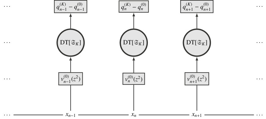 Figure 1
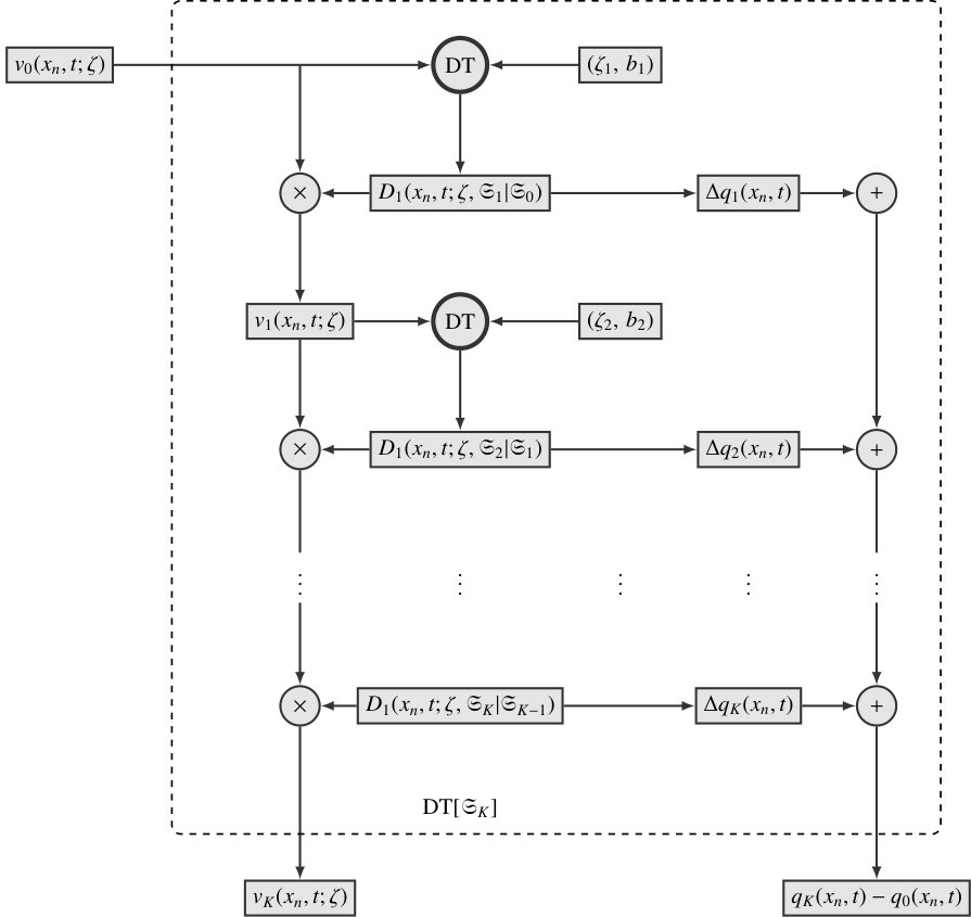 Figure 2
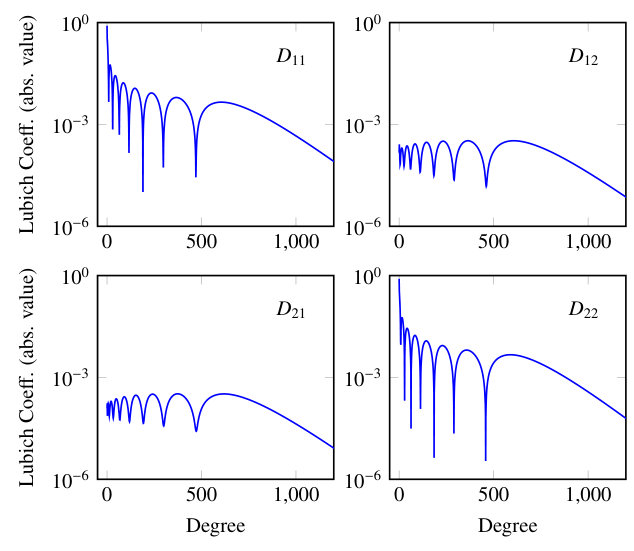 Figure 3
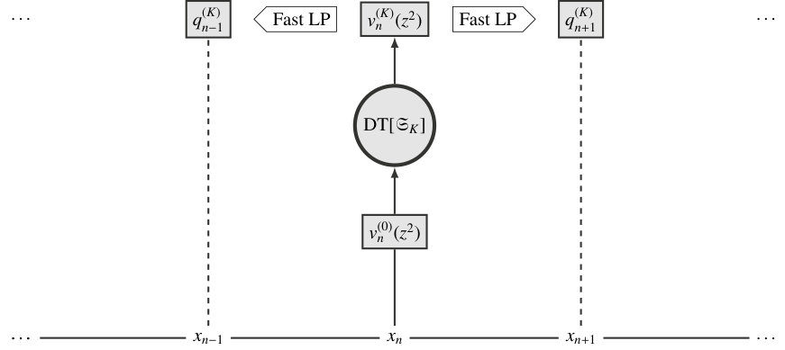 Figure 4
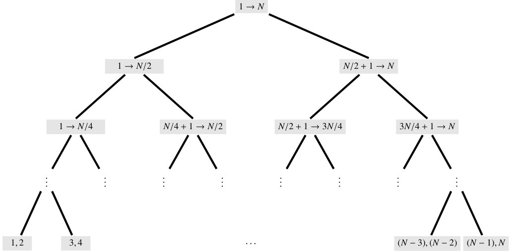 Figure 5
 Figure 6
 Figure 7
 Figure 8
 Figure 9
 Figure 10
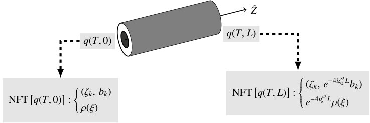 Figure 11
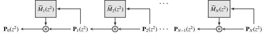 Figure 12
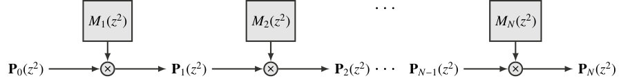 Figure 13
 Figure 14
 Figure 15
Peer Reviews
No public reviews on file for this paper yet. If you reviewed it on a platform where reviews are public (OpenReview, ICLR, NeurIPS, ICML), you can paste yours below so the community can read it here.
Videos
No videos yet. Explain this paper in a talk, walkthrough, or lecture? Add one.
Fast Inverse Nonlinear Fourier Transformation using Exponential One-Step
Methods, Part I: Darboux Transformation
V. Vaibhav
Delft Center for Systems and Control, Delft University of Technology, Mekelweg 2. 2628 CD Delft, The Netherlands
Abstract
This paper considers the non-Hermitian Zakharov-Shabat (ZS) scattering problem which forms the basis for defining the SU-nonlinear Fourier transformation (NFT). The theoretical underpinnings of this generalization of the conventional Fourier transformation is quite well established in the Ablowitz-Kaup-Newell-Segur (AKNS) formalism; however, efficient numerical algorithms that could be employed in practical applications are still unavailable.
In this paper, we present a unified framework for the forward and inverse NFT using exponential one-step methods which are amenable to FFT-based fast polynomial arithmetic. Within this discrete framework, we propose a fast Darboux transformation (FDT) algorithm having an operational complexity of such that the error in the computed -samples of the -soliton vanishes as where is the order of convergence of the underlying one-step method. For fixed , this algorithm outperforms the the classical DT (CDT) algorithm which has a complexity of . We further present extension of these algorithms to the general version of DT which allows one to add solitons to arbitrary profiles that are admissible as scattering potentials in the ZS-problem. The general CDT/FDT algorithms have the same operational complexity as that of the -soliton case and the order of convergence matches that of the underlying one-step method. A comparative study of these algorithms is presented through exhaustive numerical tests.
pacs:
02.30.Zz,02.30.Ik,42.81.Dp,03.65.Nk
Notations
The set of real numbers (integers) is denoted by () and the set of non-zero positive real numbers (integers) by (). The set of complex numbers are denoted by , and, for , and refer to the real and the imaginary parts of , respectively. The complex conjugate of is denoted by and denotes its square root with a positive real part. The upper-half (lower-half) of is denoted by () and it closure by (). The set denotes an open unit disk in and denotes its closure. The set denotes the unit circle in . The Pauli’s spin matrices are denoted by, , which are defined as
[TABLE]
where . For uniformity of notations, we denote . Matrix transposition is denoted by and denotes the identity matrix. For any two vectors , denotes the Wronskian of the two vectors and stands for the commutator of two matrices and . Partial derivatives with respect to are denoted by or while repeated derivatives by . The support of a function in is defined as . The Lebesgue spaces of complex-valued functions defined in are denoted by for with their corresponding norm denoted by or .
The inverse Fourier-Laplace transform of a function analytic in is defined as
[TABLE]
where is any contour parallel to the real line.
I Introduction
This paper considers the two-component non-Hermitian scattering problem first studied by Zakharov and Shabat (ZS) Zakharov and Shabat (1972), which forms the basis for defining the SU-nonlinear Fourier transformation (NFT). For certain integrable nonlinear equations whose general description is provided by the AKNS-formalism Ablowitz et al. (1974); Ablowitz and Segur (1981), the NFT offers a powerful means of solving the corresponding initial-value problem (IVP). One such example is the nonlinear Schrödinger equation (NSE) that is commonly used to model channels for optical fiber communication. The propagation of optical field in a loss-less single mode fiber under Kerr-type focusing nonlinearity is governed by the NSE Kodama and Hasegawa (1987); Agrawal (2013) which can be cast into the following standard form
[TABLE]
where is a complex valued function associated with the slowly varying envelope of the electric field, is the position along the fiber and is the retarded time. This equation also provides a satisfactory description of optical pulse propagation in the guiding-center or path-averaged formulation Hasegawa and Kodama (1990, 1991); Turitsyn et al. (2012) when more general scenarios such as presence of fiber losses, lumped or distributed periodic amplification are included in the mathematical model of the physical channel. The IVP corresponding to (1) consists in finding the evolved field for a given initial condition under vanishing boundary conditions.
For a given initial condition , the nonlinear Fourier spectrum consists of (i) a continuous part , and, (ii) a discrete part given by which is an ordered pair of eigenvalues and the respective norming constants (see Ablowitz et al. (1974) or Sec. II for a complete introduction). The discrete spectrum is associated with the solitonic components of the potential which will be referred to as bound states in the rest of this paper. The energy in these states does not disperse away as in the case of linear waves, a phenomenon which is adequately characterized by the term “bound states”. The evolution of the nonlinear Fourier (NF) spectrum depicted in Fig. 1 is reminiscent of evolution in a linear channel–a property which is attributed to the integrablity of the nonlinear channel.
In passing, we also note that the ZS-problem appears in various other physical systems, for instance, grating-assisted co-directional couplers (GACCs), a device used to couple light between two different guided modes of an optical fiber (see Feced and Zervas (2000); Brenne and Skaar (2003) and references therein), and, NMR spectroscopy where design of frequency selective pulses requires solution of a ZS-problem Rourke and Morris (1992a, b); Rourke and Saunders (1994).
Amongst the key physical effects that affect the performance of an optical fiber communication system, namely, chromatic dispersion, Kerr-type nonlinearity and optical noise, it is the latter two that have become the principle factors limiting the spectral efficiency of wavelength–division–multiplexed (WDM) networks at high signal powers. The reason behind this is largely the transmission methodologies that assume a linear model of the channel. The NF spectrum, in contrast, offers a novel way of encoding information in optical pulses where the nonlinear effects are adequately taken into account as opposed to being treated as a source of signal distortion. The idea to use discrete eigenvalues of the NF spectrum was first proposed by Hasegawa and Nyu Hasegawa and Nyu (1993) which they termed as the eigenvalue communication. Recently, Yousefi and Kschischang Yousefi and Kschischang (2014) have proposed nonlinear signal multiplexing in multi-user channels in order to mitigate the problem of nonlinear cross-talk that occurs in WDM systems. We note that the most general modulation technique uses both the discrete as well as the continuous part of the NF spectrum which was recently demonstrated in Aref et al. (2016). We refer the reader to a comprehensive review article Turitsyn et al. (2017) and the references therein for an overview of the progress in theoretical as well as experimental aspects of various NFT-based optical communication methodologies. It must be noted that practical implementation of NFT-based transmission is still quite far from becoming a reality Turitsyn et al. (2017) and there are other potential ways to combat nonlinear signal distortions in optical fibers Cartledge et al. (2017); Dar and Winzer (2017)111At this point, studies indicate that there is no clear winner as far as mitigation of impairments due to nonliearity in optical fibers is concerned; therefore, we continue our efforts to improve NFT-based approach. Also noteworthy is the fact that ZS-problem appears in various other systems of physical significance where this research can find application..
In any NFT-based modulation technique, the importance of low-complexity NFT-algorithms cannot be over emphasized. In this paper, we focus on the development of fast algorithms for various modulation scenarios of a NFT-based transmission system. As noted in Turitsyn et al. (2017), many of the existing numerical approaches tend to become inaccurate as the signal power increases. While this maybe attributed to lack of numerical precision, it could also be numerical ill-conditioning or as a result of naive implementation. It is difficult to fully address these problems in this work, but let us remark that stability and convergence of the numerical algorithm plays a key role in determining its performance in realistic scenarios. We discuss these two aspects quite rigorously in this work.
Our primary goal here is to provide a theoretical foundation for the algorithms reported in Vaibhav and Wahls (2017) where we also showcased our preliminary results demonstrating the first fast inverse NFT. The specific problems for which we seek fast algorithms in this work are as follows:
Problem I.1** (Generation of multi-solitons).**
Given an arbitrary discrete spectrum ( being its cardinality or, in other words, the number of bound states), compute the corresponding multi-soliton potential.
Problem I.2** (Addition of bound states).**
Given an arbitrary potential referred to as the “seed” potential (assumed to be admissible as a scattering potential in the ZS-problem) and a given discrete spectrum , compute the “augmented” potential such that its discrete spectrum is given by where is known to be disjoint with , the discrete spectrum of the seed potential.
Problem I.3** (Inversion of continuous spectrum).**
Given an arbitrary continuous spectrum , such that there exists a positive constant for which the estimate
[TABLE]
holds, compute the potential such that its continuous spectrum is and the discrete spectrum is empty.
Problem I.4** (Inverse NFT).**
Given an arbitrary continuous spectrum , satisfying the estimate in Prob. I.3 and a given discrete spectrum , compute the potential such that its continuous spectrum is and its discrete spectrum is .
The first two of these problems can be solved, at least in principle, using the Darboux transformations (DT) Lin (1990); Gu et al. (2005). The Prob. I.1 can be solved with machine precision using DT with null-potential as the seed. The resulting complexity is where is the number of eigenvalues and is the number of samples of the potential. The scenario in Prob. I.1 corresponds to the modulation of the discrete NF spectrum which has been explored by a number of groups Hari et al. (2014); Dong et al. (2015); Hari and Kschischang (2016) and it has also been experimentally demonstrated Terauchi and Maruta (2013); Bülow (2014, 2015); Matsuda et al. (2014); Aref et al. (2015); Bülow et al. (2016).
The Prob. I.2 cannot be solved without resorting to numerical methods for the ZS-problem because the so called Jost solutions (which are required in DT) are not known in a closed form for any arbitrary seed potential. Prob. I.3 and I.4 will be treated in a sequel to this paper.
The numerical techniques for solving Prob. I.1–I.4 developed in this work are based on exponential (linear) one-step methods Cox and Matthews (2002); Gautschi (2012) for the discretization of the ZS-problem. The method yields a discrete framework for solving the ZS-problem which resembles the transfer matrix approach for solving wave-propagation problems in dielectric layered media (Born and Wolf, 1999, Chap. 1). These transfer matrices have polynomial entries–a form that is amenable to the FFT-based polynomial arithmetic Henrici (1993) and is also compatible with the layer-peeling algorithm Bruckstein and Kailath (1987). All the methods considered in this article exhibit either a first order or a second order of convergence, i.e., the numerical errors vanish as where is the order of the one-step method222The discrete system corresponding to Ablowitz-Ladik (AL) scattering problem (Ablowitz et al., 2004, Chap. 3) is also amenable to FFT-based fast polynomial arithmetic and satisfies the layer-peeling property Wahls and Poor (2015a); however, it does not illuminate on how to obtain a general recipe that could be applied to the ZS-problem in order to obtained a similar discrete system possessing a given order of convergence..
Within this discrete framework, we develop two algorithms: (a) the classical Darboux transform (CDT) which addresses Prob. I.2, and, (b) the fast Darboux transformation (FDT) which addresses Prob. I.1 and I.2 both333It is worth noting that an alternative fast method of solving Prob. I.1 is reported in Wahls and Poor (2015b) and it can be readily adapted to the discrete framework considered in this work. However, this method offers no control over the norming constants, therefore, we do not address this algorithm here.. The CDT algorithm is a direct numerical implementation of the DT in the continuum case where the seed Jost solutions are computed by numerically solving the scattering problem resulting in an overall complexity of . The FDT algorithm is entirely new and it is based on the pioneering work of Lubich on convolution quadrature Lubich (1988a, b, 1994). In order to ensure compatibility with Lubich’s construction, we restricted ourselves to the implicit Euler method and the trapezoidal rule. This algorithm has an operational complexity of and an order of convergence that matches that of the underlying one-step method, i.e., where (implicit Euler), (trapezoidal rule). With increasing number of eigenvalues, FDT clearly outperforms CDT. The numerical tests and error analysis of the numerical scheme suggests that CDT is useful only for smaller number of eigenvalues. These tests further reveal that FDT is not only more accurate for the general case, it also has superior numerical conditioning with increasing number of eigenvalues as opposed to the CDT algorithm which becomes unstable.
I.1 Outline of the paper
This paper is organized as follows: In Sec. II, we summarize the basic scattering theory and the Darboux transformation in the continuous regime.
The discrete scattering framework for the ZS-problem is developed in Sec. III where the numerical discretization in the spectral domain is described in Sec. III.1, and, properties of the numerical Jost solutions are discussed in Sec. III.2. We formulate the layer-peeling scheme in Sec. III.3 which is based on the discrete framework developed in Sec. III.1. Algorithmic aspects are addressed in Sec. III.4 and III.5 where we describe the sequential algorithm and its fast version obtained using a divide-and-conquer strategy, respectively. The sections III.6 to III.8 contain the main contribution of this paper: The method of inversion of continuous scattering coefficients using the Lubich’s method is discussed in Sec. III.6. In Sec. III.7, we apply the Lubich’s method to obtain the FDT algorithm for -soliton potentials. Finally, the general version of the CDT algorithm and the FDT algorithm is discussed in Sec. III.8.
The benchmarking methods that used for comparison are discussed in Sec. IV. The necessary and sufficient condition for discrete inverse scattering is discussed in Sec. V. The stability and convergence analysis of the numerical schemes developed in earlier section is carried out in Sec. VI. The numerical experiments and results are discussed in the Sec. VII which is followed by Sec. VIII which concludes the paper.
II The AKNS System
In order to describe the fundamental basis of the nonlinear Fourier transform (NFT), we briefly review the scattering theory for a AKNS system corresponding to the NSE. Because the NSE shows up in various disciplines, we choose to present the theory in a form that is independent of the context and conform to the way it appears in the classical texts on the scattering theory. For a complex valued field , we will work with the standard form of NSE which reads as
[TABLE]
where is the evolution parameter identified as a time-like variable (this turns out to be the propagation distance for the fiber model) and is the domain over which the field is defined (which is the retarded time for the fiber model). Henceforth, we closely follow the formalism developed in Ablowitz et al. (1974); Ablowitz and Segur (1981) for the exposition in this article. The NFT of the complex-valued field is introduced via the associated Zakharov-Shabat scattering problem Zakharov and Shabat (1972) which can be stated as follows: Let and , then
[TABLE]
where
[TABLE]
is identified as the scattering potential. The second relation above corresponds to the focusing-type of nonlinearity for the NSE. The compatibility condition () between (3) and (4), assuming is independent of , produces the NSE as stated in (2).
The solution of the scattering problem (3), henceforth referred to as the ZS-problem, consists in finding the so called scattering coefficients which are defined through special solutions of (3) known as the Jost solutions described in the next subsection. These Jost solutions also play an important role in defining the Darboux transformation (DT) which is a powerful technique for constructing more complex potentials (as well as their Jost solutions) from simpler ones–this will be discussed in the final part of this section. There, we will be primarily interested in studying the form of DT which allows one to add bound states to a given potential.
II.1 Jost solutions
The Jost solutions are linearly independent solutions of (3) such that they have a plane-wave like behavior at or . In the following, we set and suppress the time-dependence of the solutions for the sake of brevity.
- •
First kind: The Jost solutions of the first kind, denoted by and , are the linearly independent solutions of (3) which have the following asymptotic behavior as : and .
- •
Second kind: The Jost solutions of the second kind, denoted by and , are the linearly independent solutions of (3) which have the following asymptotic behavior as : and .
The evolution of the Jost solutions in time is governed by the equation (4) for under the asymptotic boundary conditions prescribed above. On account of the linear independence of and , we have
[TABLE]
Similarly, using the pair and , we have
[TABLE]
The coefficients appearing in the equations above can be written in terms of the Jost solutions by using the Wronskian relations444For any pair of linearly independent vectors, , their Wronskian which is defined as
is non-zero. If also qualify as Jost solutions, then their Wronskian is independent of Ablowitz et al. (1974).:
[TABLE]
These coefficients are known as the scattering coefficients and the process of computing them is referred to as forward scattering. As it turns out, we would also be interested in studying the analytic continuation of the Jost solutions with respect to , which in turn also determines the analytic continuation of the scattering coefficients. The motivation behind this is threefold: First, the inversion of the scattering coefficients cannot be done in general by knowing the value of the scattering coefficients over the real line (i.e. ). Second, the knowledge of analyticity and decay properties of these functions in the complex plane allows us to establish certain theoretical estimates with greater ease. Lastly, in many cases, the knowledge of the analytic form introduces a certain redundancy in the system that can be exploited by the numerical algorithms to improve its numerical conditioning and stability.
In order to discuss the analytic continuation of the Jost solution with respect to , let us specify the following two classes of functions for the scattering potential (at ): Let such that or almost everywhere in for some constants and . In the former case, the Jost solutions have analytic continuation in whole of the complex plane with respect to . Consequently, the scattering coefficients , , , are analytic functions of . In the latter case, the analyticity property can be summarized as follows (Ablowitz et al., 1974, Sec. IV.A): The functions and are analytic in the half-space . The functions and are analytic in the half-space . In this case, the coefficient is analytic for while the coefficient is analytic in the strip defined by . More will be said about the analyticity and decay properties of the scattering coefficients in Sec. VI.1.
Furthermore, the symmetry properties
[TABLE]
yield the relations and .
II.2 Scattering data and the nonlinear Fourier spectrum
The scattering coefficients introduced in the last section together with certain quantities defined below that facilitate the recovery of the scattering potential are collectively referred to as the scattering data. The nonlinear Fourier spectrum can then be defined as any of the subsets which qualify as the “primordial” scattering data (Ablowitz et al., 1974, App. 5), i.e., the minimal set of quantities sufficient to determine the scattering potential, uniquely.
In general, the nonlinear Fourier spectrum for the potential comprises a discrete and a continuous spectrum. The discrete spectrum consists of the so called eigenvalues , such that , and, the norming constants such that . For convenience, let the discrete spectrum be denoted by the set
[TABLE]
For compactly supported potentials, . Note that some authors choose to define the discrete spectrum using the pair where is known as the spectral amplitude corresponding to ( denotes the derivative of ).
The continuous spectrum, also referred to as the reflection coefficient, is defined by for . The coefficient and consequently the discrete eigenvalues do not evolve in time. The rest of the scattering data evolves according to the relations and .
II.3 The Darboux transformation
The Darboux transformation provides a purely algebraic means of adding bound states to a seed solution Neugebauer and Meinel (1984); Lin (1990); Gu et al. (2005). In doing so the -coefficient of the potential remains invariant Lin (1990) while the -coefficient gets modified to reflect the addition of the bound states. In particular, starting from the “vacuum” solution (i.e. the solution for the null-potential), one can compute reflectionless potentials also referred to as the multi-soliton or, more precisely, the -soliton potential with the desired discrete spectrum. The Darboux transformation is carried out by means of Darboux matrices which is described in the following paragraphs.
Let as defined by (8) be the discrete spectrum to be added to the seed potential. Define the matrix form of the Jost solutions as
[TABLE]
The augmented matrix Jost solution can be obtained from the seed solution using the Darboux matrix as
[TABLE]
where is to be determined. In the following, we summarize the approach proposed by Neugebauer and Meinel Neugebauer and Meinel (1984) which requires the Darboux matrix to be written as
[TABLE]
where the coefficient matrices are such that (for the special case ) and
[TABLE]
From the Wronskian relation, we know ; hence, it follows that
[TABLE]
It is shown in Neugebauer and Meinel (1984) that is independent of . Further, the symmetry imposed by the condition , requires
[TABLE]
which combined with the fact that Lin (1990)
[TABLE]
yields
[TABLE]
From , we have
[TABLE]
Note that on account of , i.e., is not an eigenvalue of the seed potential. The system of equations in (10) can be used to compute the unknown coefficients of the Darboux matrix. Let and correspond to the augmented potential and the seed potential , respectively; then using the fact that is a Jost solution, we have
[TABLE]
which expands to
[TABLE]
Given that is invertible, we must have
[TABLE]
Equating the coefficient of to zero, we have
[TABLE]
II.3.1 Darboux matrix of degree one
For the sake of simplicity, let the us consider the seed solution with empty discrete spectra. Let us define the successive discrete spectra such that for where are distinct elements of .
For single bound state, described by , putting
[TABLE]
the solution of the corresponding linear system (10) yields the Darboux matrix of degree one given by
[TABLE]
The augmented potential then works out as
[TABLE]
The Jost solutions for this new potential can be obtained via the Darboux matrix and the entire procedure can be repeated for adding another bound state to the augmented potential. Suppressing the and dependence for the sake of brevity, it follows that the Darboux matrix of degree can be factorized into Darboux matrices of degree one as
[TABLE]
where are the successive Darboux matrices of degree one with the convention that is the bound state being added to the seed solution whose discrete spectra is . Using the expression in (12), we have
[TABLE]
where
[TABLE]
for and the successive Jost solutions, , needed in this ratio are computed as
[TABLE]
The successive potentials are given by
[TABLE]
See Fig. 2 for a schematic representation of the DT.
If the seed Jost solution corresponding to the seed potential is known, then the Darboux transformations can be readily carried out over any set of grid points in order to compute the augmented potential at these grid points. The resulting order of operational complexity, excluding the cost of evaluating the seed potential and the seed Jost solution, works out to be where is the number of samples of the augmented potential. For the special case of -solitons, the seed potential as well as the seed Jost solutions are trivially known; therefore, this method provides us with an algorithm for computing the -soliton potentials with machine precision. In general, closed form solutions are rarely known for arbitrary potentials; nevertheless, this procedure can be carried out with numerically computed Jost solutions in any discrete framework. This scheme will be referred to as the classical Darboux transformation (CDT) in the rest of the article. The error analysis of this method is carried out in Sec. VI.5.
For multi-solitons, the asymptotic form of the potential as works out to be
[TABLE]
and as
[TABLE]
where are the successive -coefficients. Therefore, exhibits exponential decay with a decay constant that is given by . This observation allows us to conclude that round off errors in the CDT scheme can be minimized if the eigenvalues are “added” in the decreasing order of the magnitude of their imaginary parts Vaibhav and Wahls (2016). Further, the knowledge of the decay constant can be used to choose an optimal computational domain so that the numerical errors due to domain truncation is minimized (see Sec. VII.1.1).
II.3.2 Effective support of multi-soliton potentials
A multi-soliton potential has an unbounded support, therefore, in any practical application it is mandatory to introduce an effective support with desired energy content. Posed conversely, one may also be interested in choosing the discrete spectrum which leads to a prescribed effective support with desired energy content initially or over a finite duration of evolution.
In case of multi-solitons, the energy content of the side lobe which we wish to truncate is trivially available in the CDT scheme and it can be used as a truncation criteria. Let denote the characteristic function of and let () be the domain that needs to be determined so that
[TABLE]
Suppressing the dependence on for the sake of brevity, the asymptotic expansion of with respect to yields (Ablowitz et al., 1974, Sec. IV.A)
[TABLE]
and that corresponding to yields
[TABLE]
These relationships are also known as the nonlinear Parseval’s relationships. Asymptotic estimates when can be easily obtained from the above relations:
[TABLE]
This allows us to obtain an asymptotic formula for the effective support of a -soliton potential. Define such that
[TABLE]
then
[TABLE]
under the assumption where
[TABLE]
Finally, let us note that a binary search algorithm (bisection method) can be devised to solve the nonlinear equation (14) for where can be taken as the bracketing interval for the root555Numerical tests indicates that tends to over estimate the effective support.. The complexity of such an algorithm (for fixed ) works out to be where is the number of bisection steps needed.
II.3.3 Scattering coefficients of a truncated multi-soliton
Let be taken as the point of truncation. Then a multi-soliton potential can be seen as comprising a left-sided profile (supported in ) and a right-sided profile (supported in ). The respective scattering coefficients of each of the truncated potentials turn out to be a rational function of . These observations were already made by several authors Lamb (1980); Rourke and Morris (1992b); Rourke and Saunders (1994); Steudel (2002); Steudel and Kaup (2008) and a number of different methods do exist for inversion of the scattering data which exploit the rational character of the truncated scattering coefficients. Our numerical scheme also exploits this property; therefore, we discuss this case in some detail below.
Let us consider the left-sided profile, denoted by . The Jost solution at can be computed using the Darboux transformation as described above. The Jost solution at corresponds to that of a null-potential, i.e., . The scattering coefficients for the left-sided profile, therefore, works out to be
[TABLE]
This corresponds to the first column of the Darboux matrix , therefore, a purely rational function of analytic in . Now, let us consider the right-sided profile, denoted by . The Jost solution at can be computed using the Darboux transformation as before while the Jost solution at is given by . Therefore, the relevant scattering coefficients for the right-sided profile works out to be
[TABLE]
This corresponds to the second column of the Darboux matrix and, therefore, a purely rational function of analytic in .
Remark II.1** (Conjugation and reflection).**
The inverse scattering problem for the right-sided profile can be transformed to that of a left-sided profile in the following way: putting , we have
[TABLE]
where . Denote the Jost solutions of the new system (i.e. with potential ) by , (first kind) and , (second kind), then
[TABLE]
Let , , and be the scattering coefficients for the new system, then
[TABLE]
The discrete eigenvalues do not change, however, the norming constants change as . Now, the scattering coefficients for the left-sided profile obtained as result of truncating the new potential from the right at work out to be
[TABLE]
Therefore, an implementation for the case of left-sided profile is sufficient to solve problems of general nature encountered in forward/inverse NFT.
Remark II.2** (Translation).**
Let us note that there is no loss of generality in choosing the point of truncation to be on account of the translational properties of the discrete spectrum. If we wish to choose the point of truncation to be , we can consider the transformation . Define the new potential to be so that
[TABLE]
where . Denote the Jost solutions of the new system by , (first kind) and , (second kind), then
[TABLE]
Let , , and be the scattering coefficients for the new system, then
[TABLE]
The discrete eigenvalues do not change, however, the norming constants change as .
III Discrete Forward and Inverse Scattering
In this section, we discuss certain discretization schemes for the scattering problem in (3) such that they are amenable to FFT-based fast polynomial arithmetic Henrici (1993). This method of obtaining a discrete scattering problem is referred to as the spectral-domain approach666See Bruckstein and Kailath (1987) for alternative approaches.. We begin with the transformation so that (3) becomes
[TABLE]
or,
[TABLE]
The next step is to apply linear one-step method Gautschi (2012) to (18) in order to setup a recurrence relation initialized by the given initial condition. Let us note that the method of numerical integration just described above is identified as the exponential integrator based on linear one-step methods, in particular, the integrating factor (IF) method Cox and Matthews (2002). One of the advantages of the transformation carried out above in arriving at (18) is that the “vacuum” solution obtained from the discrete problem is exact.
Remark III.1**.**
In the literature, the usage of the terms “forward scattering” and “inverse scattering” is not made precise; for instance, “forward scattering” could refer to computation of the scattering coefficients and or the nonlinear Fourier spectrum. In order to avoid any confusion arising in the usage of these terms, we follow the convention that the term “forward scattering” refers to the computation of the Jost solutions while the term “inverse scattering” refers to the process of recovering the samples of the scattering potential from (the polynomial form of) the Jost solutions. Note that in almost all cases, knowledge of the Jost solutions trivially allows one to compute the truncated discrete scattering coefficients and vice versa, therefore, no confusion should arise in what constitutes as input to the inverse scattering process.
III.1 Discretization in the spectral-domain
In order to discuss various discretization schemes, we take an equispaced grid defined by with where is the grid spacing. Define such that , . Further, let us define and treat as a fixed parameter. For the potential functions sampled on the grid, we set , where the time-dependence is suppressed. Using the same convention, and .
III.1.1 Forward Euler method
The forward Euler (FE) method is the simplest of the finite-difference schemes. It can be stated as
[TABLE]
Setting , and , we have
[TABLE]
or, equivalently,
[TABLE]
Let us note that the transfer matrix can be transformed to a form that resembles that of the implicit Euler method described in the next section: Putting , we have
[TABLE]
III.1.2 Implicit Euler method
The backward differentiation formula of order one (BDF1) is also known as the implicit Euler method. The discretization of (18) using this method reads as
[TABLE]
Setting , and , this scheme can be stated as follows:
[TABLE]
or, equivalently,
[TABLE]
III.1.3 Trapezoidal rule
The trapezoidal rule (TR) happens to be one of the most popular methods of integrating ODEs numerically. The discretization of (18) using this method reads as
[TABLE]
Setting , and , this scheme can be stated as follows:
[TABLE]
or, equivalently,
[TABLE]
III.2 Jost solutions and scattering coefficients
In order to express the discrete approximation to the Jost solutions, let us define the vector-valued polynomial
[TABLE]
The Jost solutions and , for the forward/implicit Euler method and the trapezoidal rule, can be written in the form
[TABLE]
where . Note that the expressions above correspond to the boundary conditions and which translate to and , respectively. The other Jost solutions, and , can be written as
[TABLE]
The recurrence relation for the polynomial functions defined in (25) take the form
[TABLE]
where with its inverse is determined by the respective discretization scheme. The discrete approximation to the scattering coefficients is obtained from the scattered field: yields
[TABLE]
and yields
[TABLE]
The quantities , and above are referred to as the discrete scattering coefficients. Note that these coefficients can only be defined for .
Remark III.2**.**
For the sake of brevity, we may occasionally refer to the polynomials and (as opposed to and ) as the (discrete) Jost solutions.
III.2.1 Discrete spectrum
The eigenvalues are computed by forming and employing a suitable root-finding algorithm (see Wahls and Poor (2013) and the references therein for more details). It turns out that the computation of the norming constants by evaluating is ill-conditioned on account of the vanishingly small contribution from the solitonic components of the potential. Note that addition of bound states leaves -coefficients invariant; therefore, recovery of the norming constant from cannot be expected to succeed in all cases. In order to remedy this problem, we use the general definition of the norming constants777Similar approach is reported in Hari and Kschischang (2016) and Aref (2016), however, it is not emphasized in these papers that the norming constants are never defined to be a value of unless it is guaranteed to be analytic in . Note that the study of the errors introduced by the numerical discretization also provides significant insight into why the evaluation of at complex values of is ill-conditioned (see Sec. VI.3).: To this end, we proceed by computing the truncated scattering coefficients. Consider the case of potentials truncated from the right, i.e., where is the point of truncation and is the Heaviside step function. The new potential now supported in is interpreted as left-sided with respect to . The scattering coefficient can be stated in terms of the Jost solutions of the original potential as Lamb (1980)
[TABLE]
Similarly, for potentials truncated from the left, we have
[TABLE]
Denoting the corresponding discrete scattering coefficients by , , and , where , we have
[TABLE]
where . Here can be chosen to be . Once an admissible root, , of that corresponds to a soliton is determined888Given that and , we must have ., the corresponding norming constant is obtained via the proportionality of and which translates to
[TABLE]
The truncated potential does not share discrete eigenvalues with the original potential; therefore, and . The computation of the truncated scattering coefficients can be accomplished by direct evaluation of transfer matrices and subsequently forming the cumulative product leading to an operational complexity of for each eigenvalue (see Sec. III.4.1).
It must be noted that our fast algorithm for forward scattering as discussed Sec. III.5.1 is entirely compatible with the approach suggested here. The scattering coefficients are easily obtainable from the truncated scattering coefficients using the Wronskian relations given in Sec. II.1 as
[TABLE]
Every polynomial multiplication involved above can be carried out efficiently using the FFT algorithm (see Sec. III.5.1).
III.3 Inversion of discrete scattering coefficients
In this section, we consider the problem of recovering the discrete samples of the scattering potential from the discrete scattering coefficients known in the polynomial form. This step is referred to as the discrete inverse scattering step. Starting from the recurrence relation (26), we develop a layer-peeling algorithm similar to that reported by Brenne and Skaar Brenne and Skaar (2003). The common aspect of the layer-peeling step for all kinds of discretization schemes is that using nothing but the knowledge of , one should be able to retrieve the samples of the potential needed to compute the transfer matrix so that the entire step can be repeated with until all the samples of the potential are recovered (as illustrated in Fig. 3b). In the following, we summarize the main results which facilitate the layer-peeling step corresponding to the each of the discretization schemes introduced so far. A detailed study of the recurrence relation and the proof of the necessary and sufficient conditions for discrete inverse scattering is provided in Sec. V.
III.3.1 Forward Euler method
The recurrence relation for the forward Euler method yields
[TABLE]
The layer-peeling algorithm based on the forward Euler method uses the relation
[TABLE]
where on account of (33). As evident from (19), the transfer matrix, , connecting and is therefore completely determined by (with ).
III.3.2 Implicit Euler method
The recurrence relation for the implicit Euler method yields
[TABLE]
The layer-peeling algorithm based on the implicit Euler method uses the relation
[TABLE]
where on account of (35). As evident from (22), the transfer matrix, , connecting and is therefore completely determined by (with ).
III.3.3 Trapezoidal rule
Let us assume . The recurrence relation for the trapezoidal rule yields
[TABLE]
where the last relationship follows from the assumption . For sufficiently small , it is reasonable to assume that so that (it also implies that ). The layer-peeling algorithm based on the trapezoidal scheme uses the relations
[TABLE]
where
[TABLE]
Note that and . As evident from (23), the transfer matrix, , connecting and is completely determined by the samples and (with and ).
III.4 Sequential algorithm
III.4.1 Forward scattering
The computation of the Jost solution for a given value of the spectral parameter, is considered here as the forward scattering step. The direct use of the recurrence relations obtained in Sec. VI.2 gives us a sequential algorithm (see the illustration in Fig. 3a). If , denotes the complexity of computing the Jost solution for a given , then , counting only the multiplications involved. This recurrence relation yields . It must be noted that the sequential algorithms can be useful for computing norming constants as discussed in Sec. III.2.1 if the eigenvalues are known beforehand. If good initial guesses are known for the eigenvalues, search based methods such as Newton’s method of finding the eigenvalues can also benefit from sequential algorithms Wahls and Poor (2013).
The sequential algorithm for computing the polynomial coefficients of can also be obtained in the same manner where transfer matrices are now treated as polynomial matrices. If denotes the complexity of computing the polynomial coefficients for the Jost solution , then , counting only the multiplications involved. This yields which is extremely prohibitive for large number of samples. This task can be accomplished much more efficiently using a divide-and-conquer strategy together with FFT-based fast polynomial arithmetic as described in Sec. III.5.1.
III.4.2 Inverse scattering
The inverse scattering step here refers to the retrieval of the samples of the scattering potential from the known polynomial form of the discrete scattering coefficients. This can be accomplished by a sequential layer-peeling algorithm as described in Sec. III.3 (see the illustration in Fig. 3b). If , denotes the complexity of inversion of , then counting only the multiplications. This again yields a complexity of for inverting . This task can also be accomplished much more efficiently using a divide-and-conquer strategy together with FFT-based fast polynomial arithmetic as described in Sec. III.5.2.
III.5 Fast algorithm: A divide-and-conquer strategy
III.5.1 Forward scattering
The scattering algorithm consists in forming cumulative product of, say , transfer matrices. Given that the transfer matrices have polynomial entries (of maximum degree one), one can use FFT-based polynomial multiplication Henrici (1993) to obtain a fast forward scattering algorithm. In this article we restrict ourselves to the case where is a power of . Most efficient use of the FFT-based multiplication can be made if we use a divide-and-conquer strategy as in Wahls and Poor (2015a) where products are formed pair-wise culminating in the full transfer matrix. The complexity of obtaining the cumulative transfer matrix from transfer matrices, denoted by , then satisfies the recurrence relation
[TABLE]
where is the complexity of multiplying two polynomials of degree using the FFT algorithm. The number of pairs is given by so that the recurrence relation yields
[TABLE]
which simplifies to
[TABLE]
Therefore, the complexity of the forward scattering algorithm is . Note that denotes the cost of obtaining each of the transfer matrices.
Evaluation of at an arbitrary complex point can be done using Horner’s method (Henrici, 1964, Chap. 3) which has the complexity of . However, multipoint evaluation at Fourier nodes can be carried out with complexity where is a power of .
III.5.2 Inverse scattering
In this section, we describe how to obtain a fast layer-peeling algorithm by adapting McClary’s approach McClary (1983) for our discrete inverse scattering problem. Consider the grid and let us label the segment by for . Recall that the inverse of the transfer matrix is . The cumulative transfer matrix from the -th segment to the -th segment is given by
[TABLE]
Note that in order to determine the transfer matrices for last segments starting from the -th segment, it is sufficient to have a partial knowledge of the Jost solution, more specifically999We discuss the case where the underlying one-step method is the trapezoidal rule on account of the fact that the corresponding transfer matrix is the most general among the methods considered in this article., , where denotes truncation after first coefficients. Let the complimentary polynomial vector be defined as
[TABLE]
and consider the inverse propagation relation in terms of the inverse of the transfer matrices:
[TABLE]
For every , the first two coefficients of the polynomial are required in order to determine the transfer matrix for the segment ; therefore, ensures that no contribution comes from the complimentary polynomial in computing these first two coefficients. It then follows that the transfer matrices
[TABLE]
can be determined without needing the complimentary polynomial . Once the matrices are determined, the Jost solution needed to determine the transfer matrices for segments works out to be
[TABLE]
All polynomial multiplications can be carried out using the FFT-algorithm. The observations made above makes it clear that a divide-and-conquer strategy can be easily devised in order to speed up the layer-peeling algorithm. For the inversion of the discrete scattering coefficients, we start with the associated Jost solution where is a power of , we devise a divide-and-conquer strategy that reduces the original problem into two equal size (in terms of number of segments) subproblems101010Note that the analysis in Sec. III.3 reveals that the number of coefficients associated with is exactly .. The algorithm can be described as follows:
- i.
Define a binary tree with the number of levels given by (see Fig. 4). Every parent node forks into two child nodes eventually terminating the tree at the leaf nodes. 2. ii.
Associate segments with the root node which is assumed to be at the level zero. Number of segments associated with every child node is half of that of the parent node. If denotes the number of segments associated with nodes at the -th level, then for . 3. iii.
Every node in the binary tree is labeled by the index-coordinates where is the level and being the horizontal position of the node from the left in any particular level, say , so that . If the index of the last segment associated with a given node is denoted by , then . 4. iv.
All polynomial products to be formed at any node at the -th level requires executing an FFT-algorithm for vectors of length no more than . 5. v.
The segments associated with a node dictate the associated cumulative transfer matrix and the Jost solution (with the required number of coefficients) needed in order to determine the entries of constituting transfer matrices. For the node , the associated cumulative transfer matrix is
[TABLE]
and the associated Jost solution is . 6. vi.
Our algorithm requires exactly two types of operations to be carried out at every node except for the leaf nodes. The first is the computation of the cumulative transfer matrix once the constituting matrices are known at the child nodes. The second is computing the Jost solution needed by any of the child nodes. Both of these operations boil down to polynomial multiplications, therefore, it can be carried out efficiently using the FFT-algorithm. The samples of the potential are determined at the leaf nodes.
Denoting the complexity of multiplying two polynomials of degree (via the FFT-algorithm) by , the recurrence relation for the complexity of the fast layer-peeling procedure, denoted by (where , the number of segments at level ), can be stated as
[TABLE]
The first term on the RHS corresponds to the determination of Jost solution for the second child node assuming that the Jost solution is known at the parent node and the cumulative transfer matrix is known at the first child node. The second term corresponds to the determination of the cumulative transfer matrix at the corresponding parent node using the transfer matrices of the child nodes. Observing
[TABLE]
where the last term on RHS is a correction for the root node since the determination of the cumulative transfer matrix at the root level is unnecessary. Using , we have
[TABLE]
valid for where refers to the cost of executing the leaf node. Therefore, the fast layer-peeling algorithm has the complexity of .
III.6 Inversion of scattering coefficients
Let us assume that the scattering coefficients and are analytic in such that for and some , we have
[TABLE]
where . The precise conditions under which such a situation may arise is discussed in theorems VI.2 and VI.3. We further assume that the potential is supported in a domain of the form or . In this section, we would like to develop a method to compute the discrete scattering coefficients from the analytic form of the scattering coefficients so that the corresponding inverse problem can be solved numerically using the layer-peeling algorithm discussed in Sec. III.3. It turns out that this task can be efficiently accomplished using the method developed by Lubich Lubich (1988a) which is used in computing the quadrature weights for convolution-type integrals 111111The method based on the trapezoidal rule also appears in control literature where it is known as the Tustin’s method Tustin (1947)..
Introduce the function as in Lubich (1988a) which corresponds to the A-stable one-step methods, namely, BDF1 and TR:
[TABLE]
Putting , let us define the coefficients and as
[TABLE]
The coefficients can be obtained using the Cauchy integrals
[TABLE]
which can be easily computed using FFT. Note that the zeroth coefficient can be computed exactly as
[TABLE]
On account of the decay property of the scattering coefficients with respect to , and .
Let denote either or and let represent the corresponding integrand in (50). Following Lubich (1988b), we obtain the approximation for as
[TABLE]
where . Choosing ensures that . In order to achieve an accuracy of for computing for choose and . The Lubich’s method, therefore, delivers discrete scattering coefficients with complexity excluding the cost of function evaluations.
Remark III.3**.**
If it is known that the scattering coefficients are also analytic in , say, in the strip , then Cauchy’s estimate can be used to show that the Lubich coefficients decay exponentially with . Let be such that for all . Then, Cauchy’s estimate gives
[TABLE]
where stands for or and denotes the -th Lubich coefficients.
III.6.1 Relationship with inverse Fourier-Laplace transform
In case of rational scattering coefficients, the Lubich coefficients and can be computed using the inverse Fourier-Laplace transform of the scattering coefficients. For rational functions121212It suffices for our purpose to consider rational functions with simple poles (See III.7)., resolution into partial fractions offers a straightforward means of computing inverse Fourier-Laplace transform. This property can be exploited to lower the cost of computing the discrete scattering coefficients as follows: Define the functions and as
[TABLE]
Note that for , the contour can be closed in and the integrals would evaluate to zero, therefore and are causal. According to (Lubich, 1988a, Theorem 4.1), the coefficients and approximate the quantities and up to , respectively, for (note that the zeroth coefficient is given by (51) which merely requires function evaluation). For the trapezoidal rule, this property is proven in Appendix A. It is observed that agreement between true Lubich coefficients and those computed as stated above improves with increasing . Therefore, one should choose where is a suitably chosen threshold in order to switch to the partial-fraction variant of computing Lubich coefficients.
III.7 Inversion of rational scattering coefficients: Truncated multi-solitons
In order to obtain a fast version of the Darboux transformations (DT) for generating multi-solitons (Problem I.1), we would like to employ the scattering coefficients obtained as a result of truncation of a -soliton potential at . As shown in Sec. II.3.3, the scattering coefficients are rational functions of with no poles in . Therefore, the Lubich’s method of obtaining discrete scattering coefficients as described in Sec. III.6 is also applicable here. It must be noted that in order to obtain the complete -soliton potential at a given time , the truncation must be done after computing the time-evolved Darboux matrix.
Discrete inverse scattering proceeds by computing the polynomial vector associated with the discrete scattering coefficients. Without the loss of generality, we assume that the truncation is done at (see Remark II.2). Let the discrete spectrum of the -soliton be as defined in Sec. II.2. Using the notations introduced in Sec. II.3.1 (we drop the dependence of the Darboux matrices on for the sake of brevity) and setting , for the left-sided profile, we have
[TABLE]
where truncation after terms is implied by the notation . This determines for . The right-sided profile can be generated using the transformation described in Remark II.1 so that
[TABLE]
This would determine for . Combining the two parts determines the complete multi-soliton potential. Note that the foregoing description also applies to any set of rational functions which qualify as scattering coefficients of a left-sided or a right-sided profile, respectively.
The operational complexity of this algorithm can be computed by taking into account the complexity of DT at , which is , and the complexity of computation of Lubich coefficients which is where is the number of nodes used in evaluating the Cauchy integral. Given that and , the overall complexity of generating the multi-soliton including the layer-peeling step works out to be . The algorithm presented in this section is referred to as the fast Darboux transformation (FDT) algorithm. As pointed out in Sec. II.3.1, the CDT algorithm offers machine precision for computing -soliton potentials with an operational complexity of . The fundamental difference between the CDT and the FDT algorithm is depicted in Fig. 5 where it is evident that by avoiding DT-iterations at each of the grid points (except at ) and using the fast LP algorithm, a lower complexity order algorithm can be obtained.
For any rational function, if the poles and residues are known then resolution into partial fractions offers a straightforward means of computing the inverse Fourier-Laplace transform. Let us apply this idea to the problem of generating multi-solitons as discussed in the last paragraph: Poles of the Jost solutions are known to be (where are the discrete eigenvalues), therefore, the resolution of the Darboux matrix into partial fractions reads as
[TABLE]
The inversion of leads to terms of the form , therefore, the quantities must be computed beforehand. Excluding the cost of computing the exponentials, the complexity of this algorithm is where is the number of samples in the -domain. In practice, replacing Lubich coefficients with that obtained by resolution into partial-fractions leads to increase in error and even failure to converge; however, for larger values of the index, the agreement between the two improves allowing us to reduce the overall complexity of computing the discrete coefficients by switching to the faster algorithm for where is a suitably chosen threshold131313A recipe to choose based on the number of samples , the size of the computational domain and the eigenvalue with the smallest imaginary part is provided in the Appendix A..
Before we conclude this section, it is worth mentioning that the case treated by Rourke et al. Rourke and Morris (1992b); Rourke and Saunders (1994) of rational reflection coefficient proceeds by reducing the problem to an equivalent problem of generating multi-solitons on a given half-space. Therefore, such cases are amenable to the method discussed in this article.
III.8 General Darboux transformation: Addition of bound sates
In this section, we address Problem I.2 introduced in the beginning of this article. To this end, let us note that the general Darboux transformation consists in adding a given discrete spectrum (as defined in Sec. II.2) to a given seed potential, , which is assumed to be admissible as a scattering potential in the ZS-problem. The two algorithms developed for this purpose, namely, the classical Darboux transformation (CDT) and the fast Darboux transformation (FDT) meant to carry out the general Darboux transformation are described in the following subsections. For the sake of brevity of presentation, we restrict ourselves to the case .
III.8.1 The CDT algorithm
The basic idea behind the CDT algorithm is described in Sec. II.3.1 and also depicted in Fig. 5a. In the discrete framework developed in Sec. VI.2, the seed Jost solutions (which need to be evaluated at the eigenvalues to be added) can be computed via the sequential algorithm discussed in Sec. III.4.1. Using the notations introduced in Sec. II.3.1 and Sec. III.2.1, and, introducing as the discrete approximation to , we have
[TABLE]
where , and . Noting that , the rest of the steps involved are similar to that discussed in Sec. II.3.1.
The operational complexity of computing the seed Jost solutions at eigenvalues using the sequential algorithm is so that the overall complexity of the CDT algorithm is . A final remark that we would like to make with regard to the CDT algorithm is that numerical computation of the Jost solutions for complex values of the spectral parameter tends to become inaccurate on account of the -dependence of the truncation error coefficient as discussed in Sec. VI.2. It is therefore recommended that is kept below a certain threshold.
III.8.2 The FDT algorithm
The fundamental idea of the FDT algorithm is the same as that described in Sec. III.7 which is considers the problem of adding bound states, described by , to a null seed potential. The difference merely lies in how we compute the seed Jost solutions required in the DT-iterations at for a general seed potential. Following Sec. II.3.1 and III.2.1, note that evaluation of the Jost solutions at amounts to evaluating the approximating polynomial at (setting and ), so that the recursive step for computing the -coefficients reads as
[TABLE]
where we have assumed for simplicity and . Noting that , other steps of the iteration are identical to that described in Sec. II.3.1. Here, our objective is not to follow the conventional Darboux transformation but merely obtain the truncated scattering coefficients (for the left-sided and the right-sided potential) at the origin so that a fast layer-peeling algorithm can be used to compute the samples of the augmented potential.
The operational complexity of this algorithm can be worked out as follows: The cost of computing the Jost solutions (as a polynomial vector) is and the cost of evaluation of the Jost solutions using Horner’s scheme is for each of the eigenvalues so that the overall complexity of computing the discrete truncated scattering coefficient at is where is the number of nodes used in evaluating the Cauchy integral, is the number of samples of the potential and is the number of eigenvalues to be added. Observing that , and , the overall complexity is effectively including the layer-peeling step.
The convergence behavior of the FDT algorithm is studied in the Sec. VI.5 where it is shown that the Darboux matrices can be computed with the same order of accuracy as that of the underlying one-step method used in the computation of the Jost solutions of the seed potential. Further, the global order of convergence matches that of the underlying one-step method for the computation of Lubich coefficients or the layer-peeling algorithm depending on which of the two is lower.
Finally, let us conclude this section by pointing out that if a fast and sufficiently accurate means of inversion of continuous spectrum (i.e., no bound states present) is available then a fast inverse scattering algorithm can be easily obtained for the general cases using the FDT algorithm outlined in this section. The first results in this direction are reported in Vaibhav and Wahls (2017) where the trapezoidal rule is used to develop two algorithms of complexity that exhibit a convergence behavior of .
IV Benchmarking methods
In this section, we discuss two of the conventional methods which are widely used for solving scattering problems. We would like to benchmark our method against these known methods. Unlike the linear one-step methods, here we employ a staggered grid configuration given by such that .
IV.1 Magnus integrator
By applying the Magnus method with one-point Gaussian quadrature (see Magnus (1954); Iserles and Nørsett (1999); Hochbruck and Lubich (2003)) to the original ZS-problem in (3), we obtain
[TABLE]
The exponential operator can be computed exactly as
[TABLE]
where where and . We refer to this integrator as “MG1” signifying Magnus integrator with one-point Gauss quadrature. This method is also referred to as the exponential mid-point rule in the literature and it can be shown to be consistent and stable with an order . Additionally, it also forms the part of the Lie-group methods Iserles and Nørsett (1999); Hairer et al. (2006) as it retains the SU structure of the Jost solution for . It must be noted that this method is specially suited for highly oscillatory problems and has been employed by several authors to solve forward scattering problems Boffetta and Osborne (1992); Burtsev et al. (1998). Finally, let us mention that the method of computing the norming constants as described in Sec. III.2.1 can also be adapted to MG1.
IV.2 Split-Magnus method
A further simplification obtained by applying Strang-type splitting Strang (1968) to the exponential operator provides the right discrete framework for the layer-peeling algorithm. This simplification is achieved as follows:
[TABLE]
The order of approximation is determined by applying the Baker-Campbell-Hausdorff (BCH) formula to the exponential operators (Hairer et al., 2006, Chapter 4). Setting , we have
[TABLE]
Therefore, the discretization scheme works out to be
[TABLE]
where . This form has been used by a number of authors in connection with the conventional layer-peeling algorithm Bruckstein et al. (1985); Feced and Zervas (2000); Brenne and Skaar (2003) as well as for the fast version of the layer-peeling algorithm Wahls and Poor (2015a, b). By employing the transformation , we obtain
[TABLE]
which maybe viewed as a modification of the implicit Euler scheme. The integration scheme thus obtained is referred to as the split-Magnus (SM) method. The inverse relationship is given by
[TABLE]
The Jost solution can be put in to the form
[TABLE]
where and obey the same kind of transfer matrix relation as in (26) with initial condition and . The scattering coefficients work out to be
[TABLE]
The layer-peeling property can be stated as
[TABLE]
with the following additional constraints:
[TABLE]
The norming constants can be computed using any of the following formulas
[TABLE]
Lastly, we note that a staggered grid configuration may prove superior for potentials with jump discontinuity at any grid point because the sampling of the potential at the points of discontinuity is avoided.
Remark IV.1**.**
It must be noted that the CDT and the FDT algorithms are incompatible with the staggered grid configuration, therefore, the SM integrator is ruled out for all DT-related algorithms.
V Discrete inverse scattering: Necessary and sufficient condition
In this section, we study the necessary and sufficient condition for the inversion of the discrete scattering coefficients within the framework of the numerical discretization introduced in Sec. III. Let denote a sequence of quantities such as scalars, vectors or matrices.
Definition V.1**.**
Let be a non-negative integer. A polynomial defined as in (24) (with coefficients ) is said to belong to the class if and, for all , we have
[TABLE]
with .
For any , on equating the coefficient of the zeroth degree term on LHS and RHS of (67), we obtain
[TABLE]
Therefore, and for . Note that the condition ensures that there are no constant phase factors in because the relation (67) is insensitive to constant phase factors.
Definition V.2** (Para-conjugate).**
For any scalar valued complex function, , we define . For any vector valued complex function, , we define
[TABLE]
For a matrix valued function, , we define
[TABLE]
so that the operation is distributive over matrix-vector and matrix-matrix products.
Based on the discrete formulation of the ZS-problem in Sec. III, we identified a discrete representation of the Jost solution which can also be stated in the form (leaving out the factors independent of )
[TABLE]
such that the column vectors are linearly independent for all . This implies, . In fact, the determinant must turn out to be independent of so that we may put which translates into the constraint141414Given that is a polynomial, the only way is when it is a polynomial of degree zero.
[TABLE]
For ,
[TABLE]
This condition is necessary for , defined by (68), to be a Jost solution. Further, it is easy to verify that satisfies the relation
[TABLE]
Finally, let us note that forms a -valued sequence for .
The discrete scattering problem will be assumed to be stated in the form of a recurrence relation which reads as
[TABLE]
where is a polynomial matrix of degree one. Note that as defined by (68) satisfies the relation ; therefore, in order that be a Jost solution, we must have . This relationship expands to
[TABLE]
and where is independent of . Introducing the functions
[TABLE]
it follows that the general form of the transfer matrix (of degree one in ) can be written as
[TABLE]
with
[TABLE]
Let the inverse of be denoted by which also satisfies a similar symmetry relation as in (72) and
[TABLE]
so that . Further, it is straightforward to verify that, for , the matrices and are elements of . The discrete scattering problem in its unitary form reads as
[TABLE]
Introducing , the independent elements of transfer matrix can be put into the form
[TABLE]
so that
[TABLE]
Setting , the transfer matrix admits of the following factorization
[TABLE]
For the cases considered in this article, , therefore, we assume so that it does not play a role in the unitary form of the transfer matrix for . For a given initial condition and fixed sequence of transfer matrices, the recurrence relation (71) leads to a unique polynomial associated with the Jost solution . In particular, the following result is straightforward:
Lemma V.1**.**
Let be a finite positive integer. Let the vectors and define through (79). Let , then the recurrence relation (71) determines a sequence of Jost solutions such that for every () there exists a unique polynomial associated with .
Now let us consider an arbitrary polynomial satisfying (69) for . Assume and let be associated with . To understand the properties of the polynomial , we consider the recurrence relation (71). Equating the coefficients of the zeroth degree term on the RHS and the LHS of (71), we have
[TABLE]
It is straightforward to see that
[TABLE]
and
[TABLE]
Therefore, in order that where , we must have
[TABLE]
Lemma V.2**.**
Under the assumption of the previous lemma, setting , the polynomial if and only if the sequence satisfies the constraint for . If , then .
Proof.
Using the recurrence relation (80) and the property (81) for all , it is straightforward to see that
[TABLE]
for while . The proof of the first part of the lemma follows from this relation.
For the second part, equating the coefficients of on the RHS and the LHS of (71), we have
[TABLE]
for . These relations yield
[TABLE]
for while and . Therefore, if then for . ∎
Next we would like to analyze the inverse problem described as follows: Given an arbitrary polynomial associated with satisfying
[TABLE]
for such that . Find a polynomial associated with and a transfer matrix of the form (79) such that , defined by
[TABLE]
is a Jost solution. If such a polynomial exists then it must be consistent with the recurrence relation
[TABLE]
or, equivalently,
[TABLE]
Equating the coefficient of on the RHS of (86), we have
[TABLE]
which yields the recurrence relation (81). Equating the coefficients of on the RHS and the LHS of (86), we obtain
[TABLE]
This yields
[TABLE]
and
[TABLE]
which thanks to (78) () becomes identical to (80). Note that the relationship (89) can also be verified by equating the coefficients of on the RHS and the LHS of (87):
[TABLE]
This yields
[TABLE]
which is identical to (89) thanks to (78). Now, using (89) and (90), we have
[TABLE]
where
[TABLE]
So far we have found that the parameter of must be set according to (81) so that we may write
[TABLE]
where is known but is still an unknown. In order to compute , we introduce a free parameter, , so that from (91), we have
[TABLE]
Now, let us observe that
[TABLE]
and
[TABLE]
so that
[TABLE]
Now, the zeroth degree coefficient given by (93) simplifies to
[TABLE]
Therefore, in order that where , we must have
[TABLE]
The above condition can be enforced by setting where we restrict ourselves to the case . Under this condition, the expressions for and simplifies to
[TABLE]
and
[TABLE]
respectively. Clearly, the transfer matrix as well as the polynomial is not unique as it depends on a free parameter . Note that the parameter turns out to be merely a scale factor which does not play a role in the unitary form of the discrete scattering problem. Finally, let us observe that in order to predict the highest degree term that is non-zero in , the recurrence relation for can be considered where the zeroth degree term is so that
[TABLE]
Remark V.1**.**
In the discrete inverse scattering case, the two formulas (81) and (92) remain invariant under any scaling of the polynomial . Therefore, knowledge of either or is sufficient to determine the transfer matrix .
The discussion above regarding the discrete inverse scattering step can be summarized in the following lemma:
Lemma V.3**.**
Given where and , there exists a unique unitary matrix for and a polynomial such that
[TABLE]
Further, if , then
[TABLE]
Proof.
The first part of the lemma is evident from the discussion above. The second part follows from the inequality
[TABLE]
for . ∎
Next, we consider some of special cases where it is possible to obtain unique solution of the discrete inverse scattering problem. It is worth noting that these special cases belong to a certain choice of the values .
V.1 Case I:
Let and assume . Then the forward scattering problem described in Lemma V.1 always yields a polynomial on account of Lemma V.2.
For discrete inverse scattering, the condition amounts to . From (97), we have
[TABLE]
which yields
[TABLE]
as the admissible solution (the other root violates the positivity constraint in (96)). For this case, the expression (98) for the zeroth degree coefficient simplifies to
[TABLE]
In the Lemma V.3, we favor the case of so that number of (vector) coefficients associated with be . If the steps described in the aforementioned lemma are carried out recursively to the point , we obtain
[TABLE]
Note that on account of ; therefore,
[TABLE]
Finally, we state the main result of this section which is a now merely a consequence of the preceding lemmas applied to the case at hand:
Proposition V.4**.**
Let be an arbitrary vector. Let the transfer matrices be determined by (79) using together with given by and for . Then, corresponding to the initial condition , the recurrence relation
[TABLE]
yields a unique polynomial with such that
[TABLE]
Conversely, for any given polynomial such that
[TABLE]
there exists a unique vector which determines the the transfer matrices as stated above such that the recurrence relation
[TABLE]
starting from yields .
Putting , note that the condition
[TABLE]
corresponds to the fact that in the direct part of the last proposition. The condition above is imposed explicitly in the converse part in order to ensure .
Corollary V.5**.**
Let correspond to as in the converse part of the last proposition. Then the following estimate holds:
[TABLE]
Proof.
The proof follows from the relation (100) of Lemma V.3. ∎
We conclude this section with the discussion of the trapezoidal rule which corresponds to the case at hand. Let . In the case of trapezoidal rule, it follows from the description in Sec. III.1.3 that the coefficients and introduced in (77) satisfy
[TABLE]
with and we choose . It also follows that the quantities introduced in (77) are given by
[TABLE]
Further, we have
[TABLE]
while .
V.2 Case II:
First, let us assume that . The discussion of the forward scattering problem is identical to that of the previous case. For discrete inverse scattering, this case corresponds to . The expression for the zeroth degree coefficient (98) simplifies to
[TABLE]
As in the last section, we favor the case of in the Lemma V.3. Again, if the steps described in the aforementioned lemma are carried out recursively to the point , it is easy to conclude that
[TABLE]
The necessary and sufficient condition for discrete inverse scattering in this case can be stated as:
Proposition V.6**.**
Let be an arbitrary vector. Let the transfer matrices be determined by (79) using together with for . Then, corresponding to the initial condition , the recurrence relation
[TABLE]
yields a unique polynomial with .
Conversely, for any given polynomial there exists a unique vector which determines the the transfer matrices as stated above such that the recurrence relation
[TABLE]
starting from yields .
Corollary V.7**.**
Let correspond to as in the converse part of the last proposition. Then the following estimate holds:
[TABLE]
Secondly, let us assume that . The discussion of the forward scattering problem is identical to that of the previous case. For discrete inverse scattering, this case corresponds to . The expression for the zeroth degree coefficient (98) simplifies to
[TABLE]
Here, we favor the case of in the Lemma V.3. Again, if the steps described in the aforementioned lemma are carried out recursively to the point , it is easy to conclude that
[TABLE]
The expression for the highest degree coefficient (99), simplifies to
[TABLE]
The necessary and sufficient condition for discrete inverse scattering in this case can be stated as:
Proposition V.8**.**
Let be an arbitrary vector. Let the transfer matrices be determined by (79) using together with for . Then, corresponding to the initial condition , the recurrence relation
[TABLE]
yields a unique polynomial with .
Conversely, for any given polynomial there exists a unique vector which determines the the transfer matrices as stated above such that the recurrence relation
[TABLE]
starting from yields .
Corollary V.9**.**
Let correspond to as in the converse part of the last proposition. Then the following estimate holds:
[TABLE]
V.2.1 Implicit Euler method
Let . For the implicit Euler method, it is evident from the discussion in Sec. III.1.2 that
[TABLE]
and
[TABLE]
Further,
[TABLE]
V.2.2 Split-Magnus method
For the split-Magnus method, we consider the samples on a staggered grid so that . It is evident from the discussion in Sec. IV.2 that
[TABLE]
and
[TABLE]
Further, .
V.2.3 Forward Euler method
Let . For the forward Euler method, it is evident from the discussion in Sec. III.1.1 that
[TABLE]
and . Further,
[TABLE]
VI Stability and convergence analysis
The main objective of this section is to carry out an error-analysis for various steps involved in the algorithms proposed in Sec. III. We first study the analyticity properties of the scattering coefficients in order to understand the difficulties involved in transitioning from the continuous to the discrete regime. In Sec. VI.2, we study the stability and convergence of the numerical scheme for forward scattering. Note that the convergence of the layer-peeling algorithm where the input is synthesized using Lubich’s method is not discussed in this work, instead, we study it empirically. The error propagation in layer-peeling procedure has been addressed in the work of Bruckstien et al. Bruckstein et al. (1986); however, on account of the underlying assumption of piece-wise constant potential, the question of convergence beyond the first order cannot be addressed in their work. We leave these aspects for future research.
Notations
The class of -times differentiable complex-valued functions is denoted by . A function of class is said to belong to , if the function and its derivatives up to order have a compact support in and if they vanish on the boundary (). Complex-valued functions of bounded variation over over is denoted by and the variation of any function over is denoted by . If , then exists almost everywhere such that (Jones, 2001, Chap. 16). Let to be equivalent to so that .
Let and . A complex-valued function is said to belong to the class if and there exists a constant such that the estimate holds almost everywhere in . Clearly, for . Define .
VI.1 Compactly supported and one-sided potentials
The Jost solution for compactly supported and one-sided potential are known to have analytic continuation into the upper-half of the complex plane Ablowitz et al. (1974); Ablowitz and Segur (1981). We detail some of these analyticity and decay properties of the Jost solutions required for our purpose. This discussion is motivated by the fact that our fast Darboux transformation (FDT) algorithm discussed in Sec. III.8.2 proceeds by computing the Jost solutions of a truncated potential which can be interpreted as one-sided (if it does not have a compact support). Further, the analyticity properties of the Jost solutions also determine the behavior of the Lubich coefficients as discussed in Sec. III.6.
We begin with a study of the modified Jost solutions defined by
[TABLE]
Let in the following unless stated otherwise. The system of equations (18) can be transformed into a set of Volterra integral equations of the second kind for the modified Jost solution :
[TABLE]
where with
[TABLE]
and the Volterra kernel is such that
[TABLE]
with for .
Theorem VI.1**.**
Let be supported in with . Then the estimate
[TABLE]
holds with where .
Proof.
The proof can be obtained using the same method as in Ablowitz et al. (1974); Novikov et al. (1984). For fixed , let denote the Volterra integral operator in (110) corresponding to the kernel such that
[TABLE]
Consider the -norm (Gripenberg et al., 1990, Chap. 9) of given by
[TABLE]
so that . The resolvent of this operator exists and is given by the Neumann series where with . It can also be shown using the methods in Ablowitz et al. (1974); Novikov et al. (1984) that , yielding the estimate . Therefore, for any , the relationship implies, for ,
[TABLE]
The result for in (113) follows from the observation that, for , where . Therefore, can be chosen to be . For the case of (113), we consider . The Volterra integral equations then reads as :
[TABLE]
where and the Volterra kernel is such that
[TABLE]
with for . Using the approach outlined above, it is possible to show that, for , . The result for the case in (113) then follows from the observation that for . ∎
Theorem VI.2**.**
Let with support in such that for . Then, there exists a constant independent of such that the estimate
[TABLE]
holds.
Proof.
Consider the first term on the RHS of (110): Integrating by parts, we obtain
[TABLE]
so that
[TABLE]
Setting , we have
[TABLE]
Again, integrating by parts, we have
[TABLE]
so that
[TABLE]
Putting , then
[TABLE]
Now, proceeding as in the proof of Theorem VI.1, we conclude that the estimate (119) holds with where .
∎
Finally, let us extend the preceding two results to the one-sided potentials:
Theorem VI.3**.**
Let for some with . Let and be the constant such that . Then, for every , the estimate
[TABLE]
holds with constants and given by
[TABLE]
where and .
In addition, if , then there exists a constant independent of such that the estimate
[TABLE]
holds.
VI.1.1 Error due to domain-truncation
For the purpose of numerical solution of the ZS-problem posed on a unbounded domain, it is mandatory to choose a computational domain that is bounded. This requires truncation of the original unbounded domain to a bounded domain, say, where . Let us observe here that the estimates obtained in Theorem VI.3 can be improved slightly in order to give us a better control of the domain truncation error. Let denote the Volterra integral operator corresponding to the kernel for defined in (112). Set the domain to be and assume the conditions stated in the first part of Theorem VI.3 to be true. Then it can be shown that, for , we have
[TABLE]
Now in any numerical scheme, one would take as the initial value for the Jost solution at . This step introduces an error which is bounded by . Let be a free parameter and assume . Now, if we require the maximum error to be equal to , then it suffices to have which works out to be
[TABLE]
Similar result can be obtained for truncation from the right side by using the property in Remark II.1.
VI.2 Discretization in the spectral domain
Let the grid points be as defined in Sec. III.1. In this section we discuss of the stability and convergence properties of the numerical methods developed in Sec. III.1. To this end, we closely follow the terminology introduced in Gautschi (2012) adapted to the problem at hand.
The general form of a one-step method for (18) can be stated as
[TABLE]
where dependence on the spectral parameter, , is suppressed. We keep the spectral parameter fixed in the following discussion or allow it to vary over any compact domain of . The function is referred to as the update function of the one-step method. The truncation error of this method is defined as
[TABLE]
with . A method is called consistent if . The necessary and sufficient condition for consistency in this case is . A method is said to have an order if, for some vector norm , holds uniformly over where is a compact set and is independent of , and . Let represent the grid. Let us introduce a vector-valued grid-function as where such that value of at is . The class of such solutions is denoted by . Define the infinity-norm of any grid-function as
[TABLE]
In order to introduce the concept of stability of the one-step method, let us define the residue operator as
[TABLE]
for any grid-function and (we set ). A method is said to be stable if there exists a constant for such that for any two arbitrary grid-functions, , we have
[TABLE]
for all .
Remark VI.1**.**
The intuition behind this definition, as explained in Gautschi (2012) is as follows: if denotes the grid-function obtained by the one-step method using infinite-precision arithmetic (so that ) and if denotes the grid-function obtained using finite-precision arithmetic (initial conditions being the same, i.e., ), then any stable method must yield where is the machine precision in the latter case.
Let , then there exist a constants and independent of and such that for all , (where is the induced matrix norm). This shows that for any two arbitrary vectors, and , the Lipschitz condition,
[TABLE]
is satisfied. Therefore, the stability of the one-step method (123) easily follows from (Gautschi, 2012, Theorem 5.3.1). Further, for any grid-function , we have
[TABLE]
Then using the inequality , it follows that which also guarantees the boundedness of the numerical solution when computed using infinite precision.
Finally, consistency and stability for any given one-step method imply global convergence. Moreover, if , denotes the grid-function determined by the exact solution and be any grid-function obtained using the one-step method (123) with initial condition , then where is the order of the one-step method (Gautschi, 2012, Theorem 5.3.2).
VI.2.1 Implicit Euler method
Continuing from Sec. III.1.2, we have
[TABLE]
which determines the update function to be
[TABLE]
It is easy to verify that , therefore, the method is consistent. Using the Taylor’s theorem
[TABLE]
where and . Assuming that , we have , therefore, the order of the method is . If the Jost solution under consideration is , then is bounded for (see Theorem VI.1), consequently, the truncation error coefficient to the leading order in is . Evidently, the method is stable which together with its consistency imply convergence (with order ).
VI.2.2 Trapezoidal rule
Continuing from Sec. III.1.3, we have
[TABLE]
so that the update function is given by
[TABLE]
Again, it is easy to verify that , therefore, the method is consistent. Using the Taylor’s theorem
[TABLE]
with . Assuming that , we have
[TABLE]
therefore, the order of the method is . Again, if the Jost solution under consideration is , then is bounded for (see Theorem VI.1), consequently, the truncation coefficient to the leading order in is . Evidently, the method is stable which together with its consistency imply convergence (with order ).
VI.2.3 Split-Magnus method
For the convergence analysis of the split-Magnus method described in Sec. IV.2, let us observe that an equivalent form of the integrator is
[TABLE]
Using Taylor’s theorem for matrix functions, we have
[TABLE]
with . Assuming to be twice differentiable on , we conclude that the order of the method is . Further, this one-step method is consistent and stable, therefore, also convergent for fixed (or varying in a compact domain). The truncation error coefficient to the leading order in is . This value can be seen to be twice as small as that of the trapezoidal rule. Let us note that it does not seem straightforward to determine which of the two one-step methods has smaller total truncation error coefficient (for fixed ); however, the trapezoidal rule appears to exhibit smaller total truncation error in the numerical tests.
VI.3 Computation of norming constants
In Sec. III.2.1, it was stated that the computation of norming constants from the discrete -coefficients is ill-conditioned. This can be attributed to the nature of the truncation error coefficients in the underlying one-step method for complex values of . It is evidenced by the presence of a factor of the form in the truncation error coefficient which tends to grow for (see Sec. VI.2). Therefore, it is better to “truncate” the scattering potential at the origin151515If the growth behavior of the potential is known before-hand, then it possible to choose an optimal point of truncation. and solve the corresponding one-sided ZS-problems as discussed in Sec. III.2.1. Finally, let us note that there are other discretization schemes such as the exponential time-differencing (ETD) scheme Cox and Matthews (2002) which may alleviate these problems; however, it may come at a cost of increased operational complexity. These ideas will be explored in a future publication.
VI.4 Lubich’s method
Starting from the functions and analytic in the upper-half of the complex plane, Lubich’s construction as described in Sec. III.6 allows us to compute the polynomials associated with the discrete scattering coefficients . Note that, in the preceding section, we discussed the necessary and sufficient condition for discrete inverse scattering with polynomials (which can be seen as a finite-support sequence of coefficients). However, Lubich’s method yields infinite series that needs to be truncated. Therefore, the compatibility of Lubich’s construction with the layer-peeling algorithm cannot be studied within the framework of finite-support sequences. However, it is possible to determine if can be associated to a Jost solution prior to truncation of the series. If the coefficients of the series decay sufficiently fast, the truncation introduces a negligible error so that the layer-peeling criteria can be satisfied to a sufficient degree of accuracy.
Let us first consider the case of compactly supported potential. Define the vector as
[TABLE]
which can be expanded into a convergent Taylor series as in Sec. III.6 on account of the analyticity of the scattering coefficients over whole of the complex plane. Further note that
[TABLE]
Therefore, for , we have161616For sufficiently small , it can be verified that . Other conditions pertaining to the specific discretization schemes can be explicitly verified using the results in Sec. III.6.
[TABLE]
Note that here we have used the fact that for all , however, such a relationship would not hold if we relax the requirement of compact support of the potential.
Let denote either or . When is analytic in the upper-half of the complex plane, then on any compact domain the functions can be regarded as Lipschitz continuous. Observing that where for BDF1 and for TR, we have
[TABLE]
on any compact domain of and () where depends only on and . Therefore, using the estimate (129) and the Lipschitz continuity of one can assert that there exists a constant for a given and such that Lubich (1994)
[TABLE]
Therefore, the Wronskian relationship, for can only be satisfied upto on any bounded interval in .
Finally, as far as the truncation of the infinite series is concerned, let us note that for the kind problems considered in this article, Lubich’s method is applied to rational functions with known poles in which makes it easy to determine the decay behavior of these coefficients using the method of partial-fractions (see Sec. III.7).
VI.5 Darboux transformation
In this section, we study convergence behavior of the Darboux transformation with numerically computed Jost solutions. Continuing from Sec. II.3, let denote the discrete eigenvalue and the corresponding norming constant. Define the Vandermonde matrix
[TABLE]
the diagonal matrix and the vectors
[TABLE]
where
[TABLE]
The unknown Darboux coefficients can be put into the vector form
[TABLE]
then the linear system of equations (10) which determines the coefficients of the Darboux matrix can be written as
[TABLE]
Note that the quantities and are known exactly while (and in turn ) is determined only up to , where is the order of convergence of the one-step method. Let denote the Euclidean norm for vectors and the induced spectral norm for matrices. Define to be the condition number of ; then, under the assumption (which can be satisfied for sufficiently small ), the standard perturbation theory (Lancaster and Tismenetsky, 1985, Chap. 11) yields the estimate
[TABLE]
Given that the perturbations are of , from above equation it follows that the coefficients of the Darboux matrix can be determined up to .
In order to determine the convergence behavior of the fast Darboux transformation (FDT) algorithm as described in Sec. III.8.1, we need to study the convergence of the corresponding Lubich coefficients. To this end, let us denote by the approximation to the Darboux matrix (for the sake of brevity, we suppress the dependence on , and ). Now, using the partial fraction expansion as in (53), we have
[TABLE]
In order to establish the relationship between the error in the Darboux matrix as stated above and the error in the coefficients of the Darboux matrix, we need the following lemma:
Lemma VI.4**.**
For a given discrete spectrum where is finite, the inequality
[TABLE]
holds for any where
[TABLE]
Proof.
From the the definition of the Darboux matrix, we have
[TABLE]
for . Now, using the Cauchy-Schwartz inequality, we obtain
[TABLE]
Note that this inequality does not change on replacing the spectral norm () with the Euclidean norm () and it is easy to see
[TABLE]
which concludes the proof. ∎
Let and denote the inverse Fourier-Laplace transform of and , respectively; then, we have the following proposition for the rate of convergence:
Proposition VI.5**.**
Consider the discrete spectrum with finite . If where is order of the underlying one-step method, then
[TABLE]
Proof.
Let the set of eigenvalues be corresponding to and define
[TABLE]
where is as defined in the forgoing lemma. From (135) and the forgoing lemma, we have
[TABLE]
where . The result follows by setting . ∎
Let the matrix-valued Lubich coefficients for and be defined as
[TABLE]
respectively. The zeroth Lubich coefficient is obtained by evaluating the Darboux matrix at . Therefore,
[TABLE]
leading to . Using the properties of the Lubich coefficients and the forgoing proposition, it follows that
[TABLE]
VII Numerical Tests
In this section, we present several numerical tests to demonstrate the performance of the numerical algorithms developed in this paper. For better numerical conditioning, we scale the scattering potential of the ZS-problem by a suitable scaling parameter such that is unity or close to unity. Let us briefly review the effect of this scaling to (3): For some , let , and then
[TABLE]
where .
For the sake of clarity, let us specify the acronyms used to denote the one-step methods considered in this article for testing: implicit Euler method (BDF1), trapezoidal rule (TR), Magnus method with one-point Gauss quadrature (MG1) and split-Magnus method (SM). The main focus of this section is to study the dependence of the total numerical error on the free parameters of a given algorithm together with its total run-time. In particular, we have considered the test cases that test the performance of the new methods introduced in this article against the so called benchmarking methods (MG1 and SM) wherever possible. In all of the test cases described below, represents the number of samples which is taken from the set .
VII.1 Examples
Our test cases are derived from following examples for which the exact value of the quantities to be analyzed are known in a closed form or can be evaluated to the machine precision by a known method.
VII.1.1 Multi-solitons
Define a sequence of angles for by choosing , and
[TABLE]
so that . Then the eigenvalues for our numerical experiment are chosen as
[TABLE]
The norming constants are chosen as
[TABLE]
Here we choose, and . Then we consider a sequence of discrete spectra defined as
[TABLE]
where . Let be the set of all the eigenvalues. The potential can be computed with machine precision using the CDT algorithm which is taken as the reference for error analysis in this case. For fixed , the eigenvalues are scaled by the scaling parameter . Let , then the computational domain for this example is chosen as where .
VII.1.2 Secant-hyperbolic potential
The exact solution of the ZS-problem for the secant-hyperbolic potential was first reported in Satsuma and Yajima (1974). We summarize the results required for our purpose as follows: Let the potential be written as
[TABLE]
where is referred to as the amplitude. The scattering coefficients are then given by
[TABLE]
The eigenvalues are given by
[TABLE]
where is the largest integer smaller than . Putting , the non-integer part of , the -coefficient can be written as a product of solitonic and radiative parts as follows
[TABLE]
Note that belongs to a secant-hyperbolic potential with amplitude . The corresponding norming constants are given by .
This example allows one to test the CDT and the FDT algorithms where the seed potential can be taken as and the sequence of discrete spectra to be added,
[TABLE]
where we set . Corresponding to , the amplitude of the augmented secant-hyperbolic potential is given by and . As in the last example, for fixed , the eigenvalues are scaled by the scaling parameter given by .
In order to choose the computational domain for the sech-potential (142) with the aforementioned scaling, we can use the relation (122). Choosing where is the set of all the eigenvalues and observing that
[TABLE]
we have which rounds to for .
VII.2 Test cases
VII.2.1 Discrete spectrum
For multi-soliton potentials described in Sec. VII.1.1, we test the convergence behavior with regard to the discrete spectrum for various discretization schemes, namely, BDF1, TR, SM and MG1. For the convergence behavior of the numerically computed norming constants, we assume that the eigenvalues are known exactly. The error in the norming constants is quantified by
[TABLE]
For the convergence behavior with regard to the eigenvalues, we compute where the -coefficient is computed numerically. The error is then quantified by
[TABLE]
For MG1, the limit is evaluated by setting . For others . Except for MG1, all other schemes are implemented using the fast forward scattering algorithm (see Sec. III.5.1). The computation of the norming constant is discussed in Sec. III.2.1 and Sec. IV.
VII.2.2 Multi-soliton potential
In this test case, we carry out the convergence analysis and a comparison of run-time (per sample) of different variants of the FDT algorithm for multi-solitons as described in Sec. VII.1.1. Note that the CDT algorithm in this case gives the exact potential which allows us to compute the total numerical error for the FDT algorithm for arbitrary discrete spectra. The error is quantified by
[TABLE]
where the integrals are evaluated numerically using the trapezoidal rule.
The different variants of the FDT algorithm are described as follows: any one-step method for the ZS-problem can be combined with any one-step method for the Lubich coefficients to obtain the FDT algorithm. In particular the relevant combinations are: BDF1-BDF1, BDF1-TR and TR-TR. We also consider the partial-fraction variant of the TR-TR combination which is labeled as TR-TR-PF. Note that the combination of a first order method for the ZS-problem with a second order method for the Lubich coefficients or vice versa should lead to a first order FDT algorithm. A second order method for the ZS-problem must be combined with a second order method or higher for the Lubich coefficients in order to obtain a second order FDT algorithm.
Parameters for the Lubich method are as follows: and (for the PF-variant). For the Cauchy integral, the radius of the circular contour is .
VII.2.3 General Darboux transformation
In this test case, we carry out the convergence analysis and a comparison of run-time (per sample) of different variants of the CDT/FDT algorithm for the secant-hyperbolic potential as described in Sec. VII.1.2. Note that, in the case of the secant-hyperbolic potential, the soliton-free seed potential as well as the augmented potential can be stated in a closed form.
The variants of the CDT/FDT algorithm are determined by the underlying one-step method. Unlike in the last test case (Sec. VII.2.2), Lubich method uses the same one-step method as that of the ZS-problem. The total numerical error is quantified by (146). Parameters for the Lubich method are the same as in the last test case.
VII.3 Results and discussion
VII.3.1 Discrete spectrum
For a given multi-soliton, this test case was designed to assess the performance of the discretization schemes, namely, BDF1, TR, SM and MG1 in the determination of the discrete spectrum. The results are plotted in Fig. 7 where it can be easily seen that all the methods considered show convergence at a rate that is determined by the underlying one-step method. However, the rate of convergence of BDF1 with regard to discrete eigenvalues seems to be better than expected as evident from the plots in the bottom row of Fig 7. The overall accuracy of MG1 is evidently superior to that of others while TR turns out to be a close second.
VII.3.2 Multi-soliton potential
This test case was designed to study the convergence and run-time behavior of different variants of the FDT algorithm for multi-solitons. The results for fixed number of eigenvalues and varying number of samples is shown in Fig. 8. The second order of convergence of the schemes BDF1-TR, TR-TR and TR-TR-PF can be identified from the plots in the top row of Fig. 8. The scheme BDF1-TR shows better rate of convergence than expected.
The run-time behavior of CDT for fixed number of eigenvalues is clearly superior to all of the method as evident from Fig. 8 (bottom row). The scheme TR-PF however becomes very competitive with the CDT algorithm.
The relative error and the run-time (per sample) as a function of the number of eigenvalues keeping the number of samples fixed is shown in Fig. 9. Here, the FDT algorithm outperforms the CDT algorithm with TR-TR-PF variant being the fastest as evident from the plots in the bottom row of Fig. 9. It is interesting to note that the relative error as a function of number of eigenvalues as shown in plots at the top row of Fig. 9 exhibits exponentially increasing behavior. This puts an upper limit to the number of eigenvalues that can be handled with the FDT algorithm within a given precision171717Note that the CDT algorithm also suffers from this drawback. However, in order to determine the upper limit for the CDT algorithm, one requires an implementation which employs a variable precision arithmetic. This program is not followed in this article..
VII.3.3 General Darboux transformation
This test case was designed to study the convergence and run-time behavior of different variants of the CDT/FDT algorithm for a soliton-free seed potential. The results for fixed number of eigenvalues (that are meant to be added) and varying number of samples is shown in Fig. 12. The second order of convergence of the TR variant of the CDT/FDT algorithm can be identified from the plots in the top row of Fig. 12. However, the TR variant of the CDT algorithm performs not only worse as compared to that of the FDT algorithm but it also becomes unstable with increasing number of eigenvalues. Further, unlike the CDT algorithm, the BDF1 and TR variant of FDT shows convergence (at an expected rate) with increasing number of samples.
The run-time behavior of CDT for fixed number of eigenvalues is clearly superior to that of FDT as evident from Fig. 13 (bottom row). The scheme TR-PF however becomes very competitive to the CDT-TR variant. Note that CDT in this case is reliable only for small number of eigenvalues.
The relative error and the run-time (per sample) as a function of the number of eigenvalues keeping the number of samples fixed is shown in Fig. 13. Here, the FDT algorithm outperforms the CDT algorithm with TR-TR-PF variant being the fastest as evident from the plots in the bottom row of Fig. 13. As in the last test case, the relative error as a function of number of eigenvalues as shown in plots at the top row of Fig. 13 exhibits exponentially increasing behavior. Note that FDT not only outperforms CDT in terms of accuracy, it also exhibits superior numerical conditioning with increasing number of eigenvalues as evident from Fig. 13 (top row).
VIII Conclusion
To conclude, we have presented a systematic approach to discretize the non-Hermitian Zakharov-Shabat (ZS) problem which is based on exponential one-step methods. The discrete framework thus obtained is amenable to FFT-based fast polynomial arithmetic and also admits of a layer-peeling property. In this setting we have presented different variants of a fast forward/inverse SU(2)-nonlinear Fourier transformation (NFT) algorithm. As a first step towards developing a general fast inverse NFT, we have presented several ways to obtain a fast Darboux transformation (FDT) algorithm with an operational complexity of where is the number of eigenvalues to be added to a seed potential and is the number of samples of the potential. This algorithm exhibits an order of convergence that matches the underlying exponential one-step method. In particular, if one uses the trapezoidal rule of integration, the order of convergence is . The strength of this algorithm was demonstrated by exhaustive numerical tests where we could successfully add eigenvalues to a soliton-free seed potential. It must be noted that the FDT algorithm shows a promising route to a fast inverse NFT which is confirmed empirically in Vaibhav and Wahls (2017)–this forms the subject matter of a sequel to this paper.
Furthermore, we have also presented a second approach that naively tries to mimic the classical Darboux transformation (CDT) scheme in the discrete framework developed for the ZS-problem with an arbitrary seed potential. This algorithm affords a complexity of ; however, it turns out to be less accurate and numerically unstable beyond certain number of eigenvalues.
Finally, let us emphasize that, based on the ideas presented in this paper and drawing on the pioneering work of Lubich on convolution quadrature, it seems plausible to anticipate the existence of higher-order convergent fast forward/inverse NFT algorithms using (exponential) linear multistep methods–we hope to return to this theme in the future.
Appendix A Lubich coefficients for rational functions with simple poles
Consider the simplest case of a rational function with a simple pole where . It satisfies the kind of growth estimated stated in (47). The inverse Fourier-Laplace transform is given by . The Lubich coefficients corresponding to the trapezoidal rule is defined through
[TABLE]
where we note that on account of . The Lubich coefficient is defined as the coefficient of in the RHS of (147) which can be worked out explicitly: and, for ,
[TABLE]
Note that when , then we may restrict so that where . In the following, we wish to study the error involved in replacing with . For , this difference is given by
[TABLE]
Using the -Padé approximant Baker and Graves-Morris (1981), we have
[TABLE]
Next, let us show that, for , there exists a positive integer dependent only on such that
[TABLE]
Recalling , let be chosen such that
[TABLE]
From the inequality (Olver et al., 2010, Chap. 4)
[TABLE]
it follows that . Also, observing
[TABLE]
it suffices to choose to be the smallest integer greater than . Now, using standard inequalities for exponential function (Olver et al., 2010, Chap. 4), we have
[TABLE]
where
[TABLE]
Finally, using the last estimate and from (149), we conclude
[TABLE]
where is independent of and . If in addition , then for and , we may write
[TABLE]
where is independent of and . Using this estimate, let us now show that one can make an informed choice of the parameter introduced in sections III.6.1 and III.7 in connection with the partial-fraction variant of FDT. To this end, we start with
[TABLE]
where is a positive number less than unity. Putting and using where and , we have
[TABLE]
Setting and for one can set so that . In case of multi-solitons, we would like to tune the parameter with respect to the eigenvalue with the smallest imaginary part. Here must be replaced by the complex conjugate of the eigenvalue with smallest imaginary part. For example, if the smallest of all the imaginary parts of eigenvalues is unity and , we should choose (or, so that is a power of when is a power of ).
The reference list from the paper itself. Each links out to its DOI / PubMed record.
- 1Zakharov and Shabat (1972) V. E. Zakharov and A. B. Shabat, Sov. Phys. JETP 34 , 62 (1972).
- 2Ablowitz et al. (1974) M. J. Ablowitz, D. J. Kaup, A. C. Newell, and H. Segur, Studies in Applied Mathematics 53 , 249 (1974) . · doi ↗
- 3Ablowitz and Segur (1981) M. Ablowitz and H. Segur, Solitons and the Inverse Scattering Transform (Society for Industrial and Applied Mathematics, 1981). · doi ↗
- 4Kodama and Hasegawa (1987) Y. Kodama and A. Hasegawa, Quantum Electronics, IEEE Journal of 23 , 510 (1987) . · doi ↗
- 5Agrawal (2013) G. Agrawal, Nonlinear Fiber Optics , Academic Press (Academic Press, 2013).
- 6Hasegawa and Kodama (1990) A. Hasegawa and Y. Kodama, Opt. Lett. 15 , 1443 (1990) . · doi ↗
- 7Hasegawa and Kodama (1991) A. Hasegawa and Y. Kodama, Phys. Rev. Lett. 66 , 161 (1991) . · doi ↗
- 8Turitsyn et al. (2012) S. K. Turitsyn, B. G. Bale, and M. P. Fedoruk, Physics Reports 521 , 135 (2012) , dispersion-Managed Solitons in Fibre Systems and Lasers. · doi ↗