Multi-mode Bose-Hubbard model for quantum dipolar gases in confined geometries
Florian Cartarius, Anna Minguzzi, Giovanna Morigi

TL;DR
This paper develops a multi-mode Bose-Hubbard model to study quantum phases of ultracold polar molecules in confined geometries, capturing quantum fluctuations and phase transitions at the linear-zigzag instability with limited computational resources.
Contribution
The authors derive a generalized multi-mode Bose-Hubbard model for dipolar gases in confined geometries, incorporating quantum fluctuations and analyzing phase diagrams at the zigzag instability.
Findings
Quantum fluctuations significantly influence ground state properties.
Aspect ratio of transverse trap frequencies controls quantum phases.
Model accurately captures key features with limited computational effort.
Abstract
We theoretically consider ultracold polar molecules in a wave guide. The particles are bosons, they experience a periodic potential due to an optical lattice oriented along the wave guide and are polarised by an electric field orthogonal to the guide axis. The array is mechanically unstable by opening the transverse confinement in the direction orthogonal to the polarizing electric field and can undergo a transition to a double-chain (zigzag) structure. For this geometry we derive a multi-mode generalized Bose-Hubbard model for determining the quantum phases of the gas at the mechanical instability taking into account the quantum fluctuations in all directions of space. Our model limits the dimension of the numerically relevant Hilbert subspace by means of an appropriate decomposition of the field operator, which is obtained from a field theoretical model of the linear-zigzag…
Click any figure to enlarge with its caption.
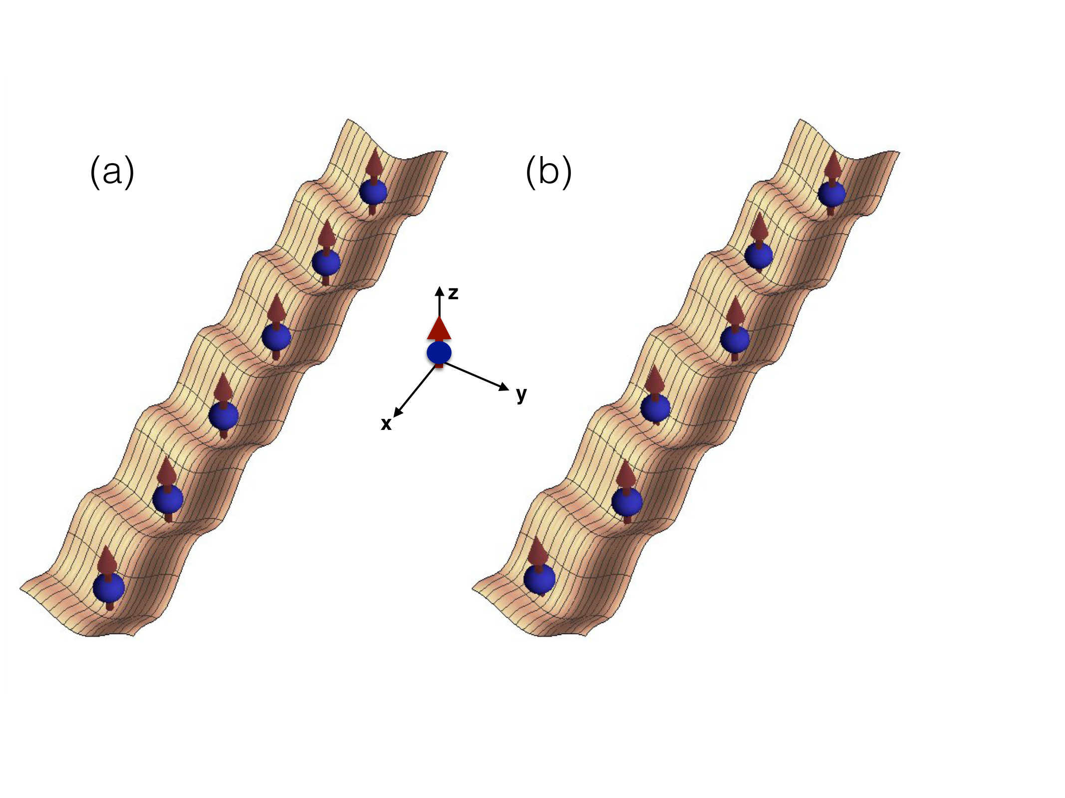 Figure 1
 Figure 2
 Figure 2
 Figure 2
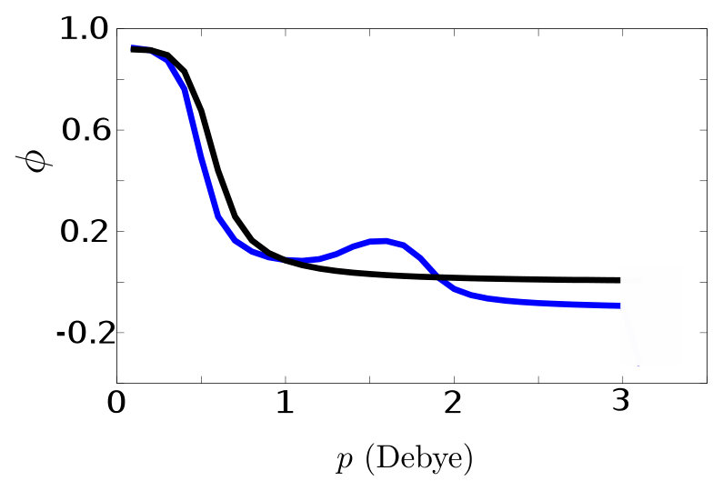 Figure 3
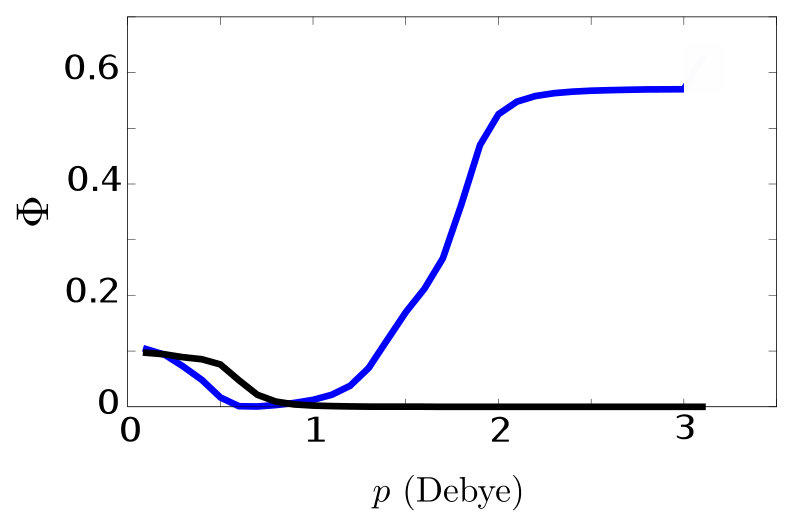 Figure 3
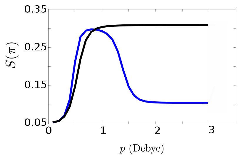 Figure 3
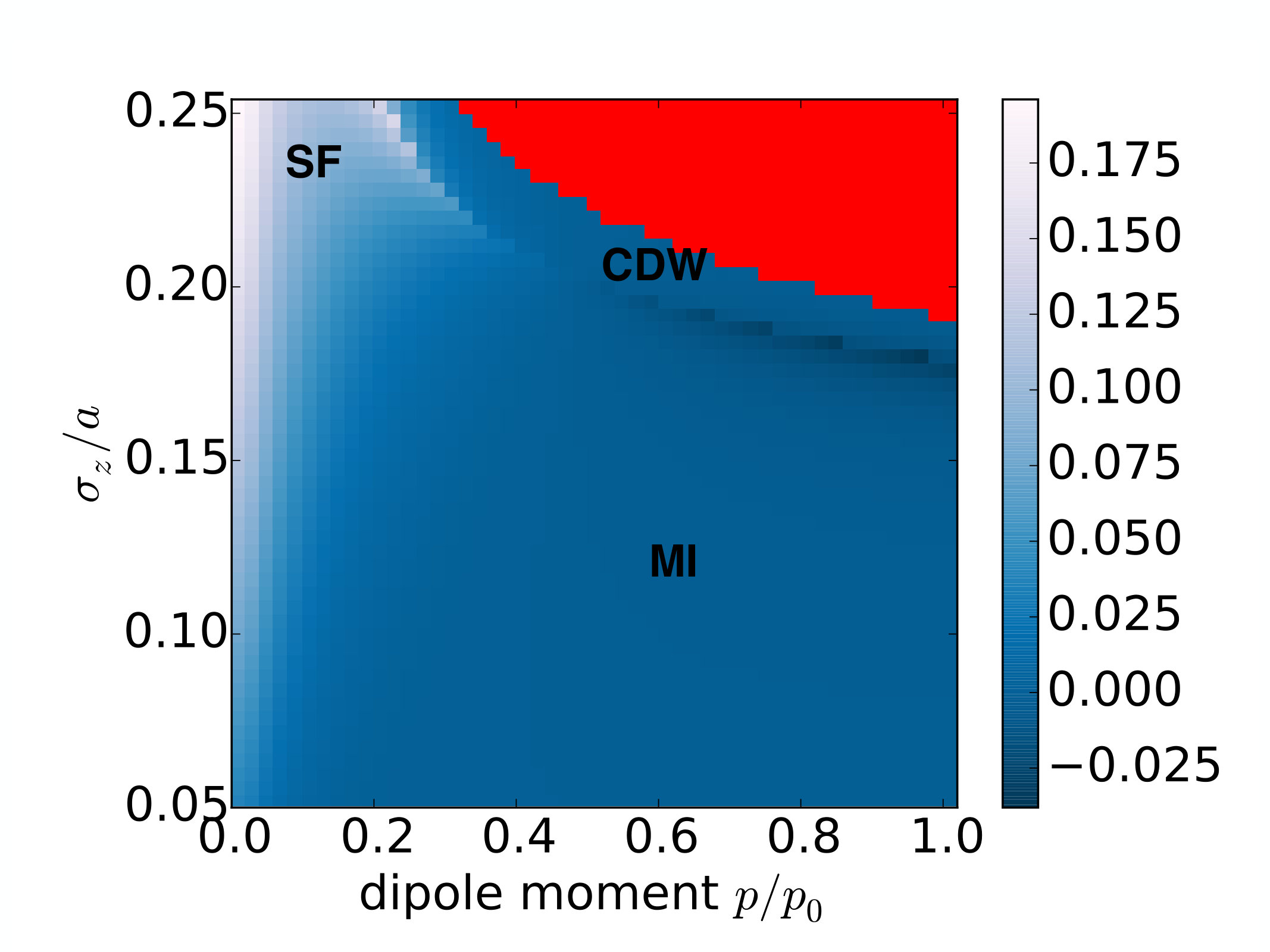 Figure 4
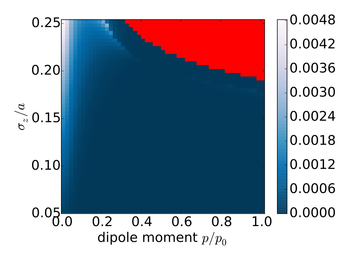 Figure 4
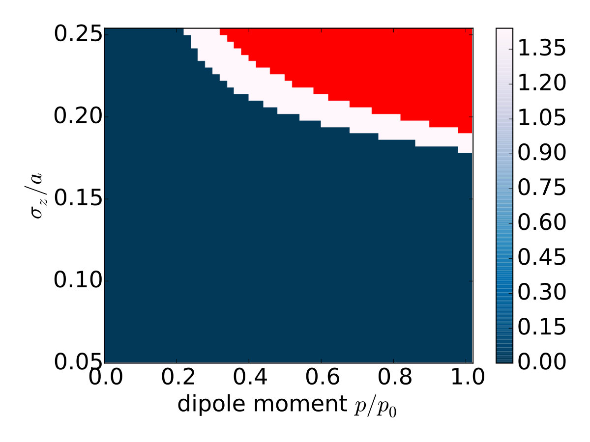 Figure 4
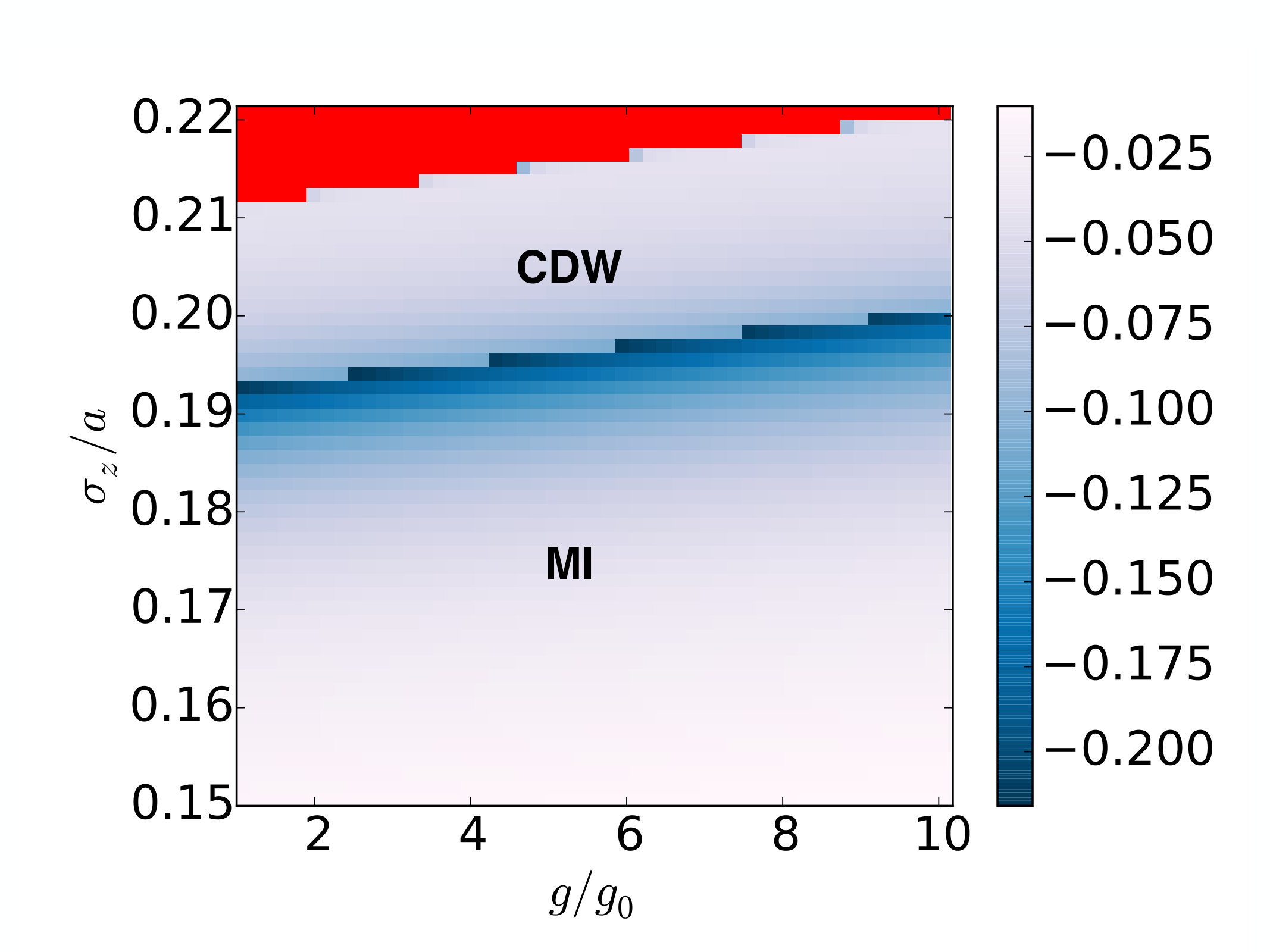 Figure 5
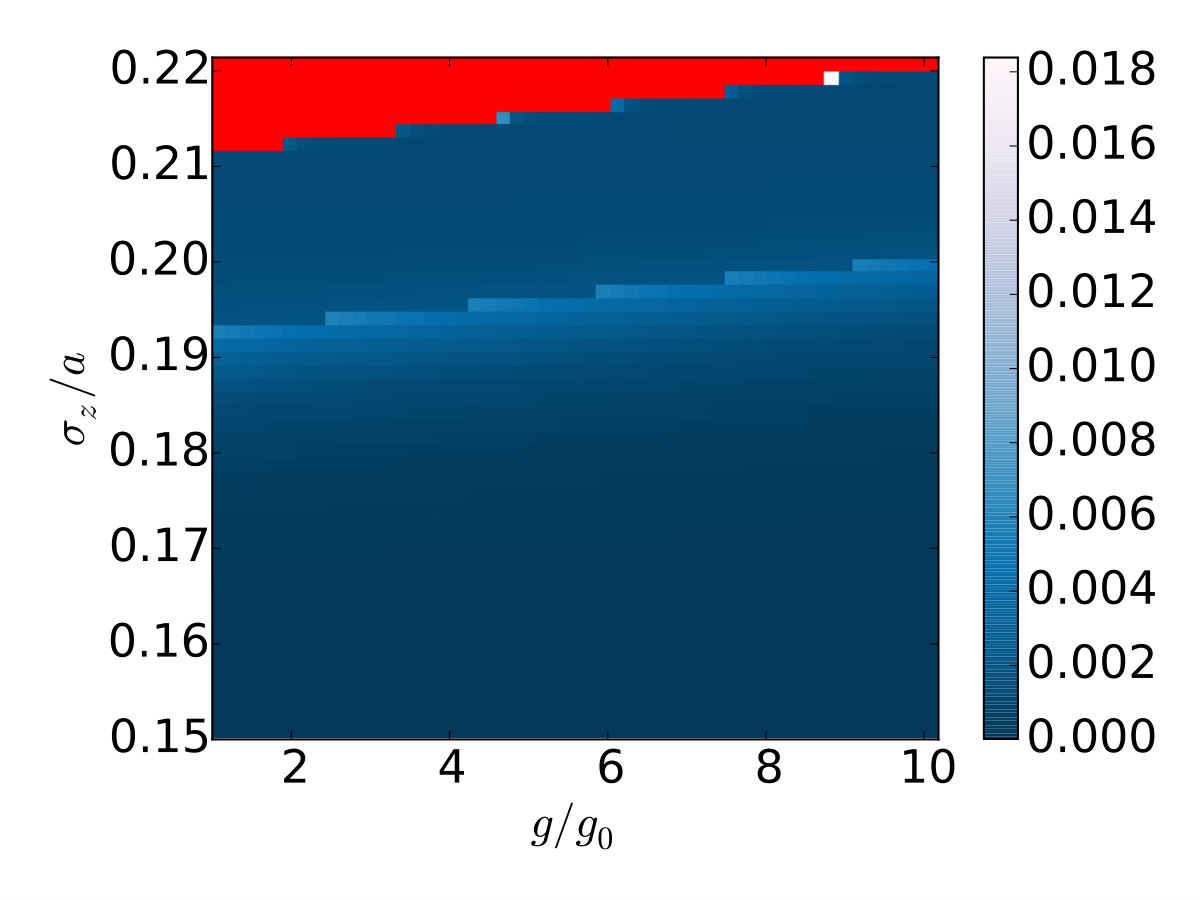 Figure 5
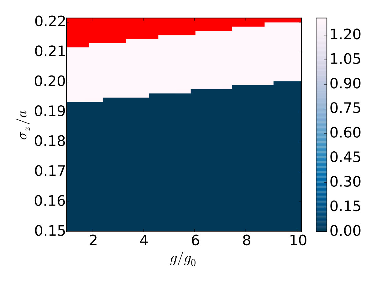 Figure 5
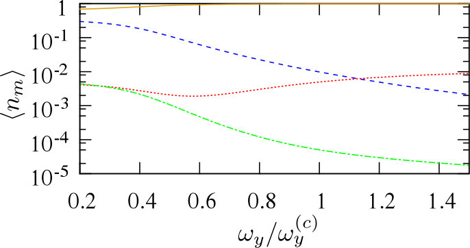 Figure 6
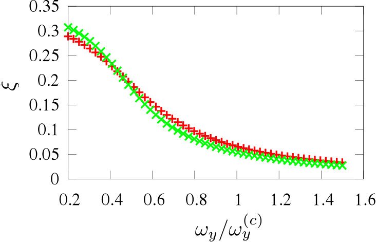 Figure 7
Peer Reviews
No public reviews on file for this paper yet. If you reviewed it on a platform where reviews are public (OpenReview, ICLR, NeurIPS, ICML), you can paste yours below so the community can read it here.
Videos
No videos yet. Explain this paper in a talk, walkthrough, or lecture? Add one.
Multi-mode Bose-Hubbard model for quantum dipolar gases in confined geometries
Florian Cartarius
Université Grenoble-Alpes, CNRS, Laboratoire de Physique et Modélisation des Milieux Condensés, 38000 Grenoble, France
Theoretische Physik, Universität des Saarlandes, D66123 Saarbrücken, Germany
Anna Minguzzi
Université Grenoble-Alpes, CNRS, Laboratoire de Physique et Modélisation des Milieux Condensés, 38000 Grenoble, France
Giovanna Morigi
Theoretische Physik, Universität des Saarlandes, D66123 Saarbrücken, Germany
(March 16, 2024)
Abstract
We theoretically consider ultracold polar molecules in a wave guide. The particles are bosons, they experience a periodic potential due to an optical lattice oriented along the wave guide and are polarised by an electric field orthogonal to the guide axis. The array is mechanically unstable by opening the transverse confinement in the direction orthogonal to the polarizing electric field and can undergo a transition to a double-chain (zigzag) structure. For this geometry we derive a multi-mode generalized Bose-Hubbard model for determining the quantum phases of the gas at the mechanical instability taking into account the quantum fluctuations in all directions of space. Our model limits the dimension of the numerically relevant Hilbert subspace by means of an appropriate decomposition of the field operator, which is obtained from a field theoretical model of the linear-zigzag instability. We determine the phase diagrams of small systems using exact diagonalization and find that, even for tight transverse confinement, the aspect ratio between the two transverse trap frequencies controls not only the classical but also the quantum properties of the ground state in a non-trivial way. Convergence tests at the linear-zigzag instability demonstrate that our multi-mode generalized Bose-Hubbard model can catch the essential features of the quantum phases of dipolar gases in confined geometries with a limited computational effort.
I Introduction
Dipolar bosonic gases offer a laboratory for studying the interplay of finite-range interactions and quantum fluctuations Lahaye ; Jin . The study of their dynamics in optical lattices, moreover, allows one to realize and characterize strongly-correlated states of ultracold matter Lahaye ; Jin ; BlochRMP ; Ferlaino2016 . The essential features of the quantum phases of ultracold dipoles in optical lattices are believed to be captured by the so-called extended Bose Hubbard Model EBH . This model reduces to the single-band Bose-Hubbard model for vanishing dipolar coupling, which at commensurate densities exhibits the Mott-Insulator to Superfluid quantum phase transition Bose-Hubbard ; BlochRMP ; FisherAndFisher . For finite strengths of the dipolar interactions, in addition, it includes a finite-range interaction term that favours the appearance of diagonal long-range order Goral ; Menotti ; Batrouni2013 ; Deng2013a ; Deng2013b ; Batrouni2014 .
In three dimensions the anisotropic nature of the dipolar interaction is reflected in the properties of the Bose-Hubbard coefficients and can be analysed by orienting the dipolar structure by means of an external field Ferlaino2016 . When the motion is confined on a plane, instead, the mutual dipolar interaction can be made effectively isotropic and repulsive by orienting the dipoles perpendicularly to the plane itself. In this regime crystalline structures can emerge from the competition between the external confinement and the particles repulsion Astrakharchik:2007 ; Buechler:2007 ; Jin .
One exemplary situation is the linear-zigzag instability. This instability can be observed by tuning the frequency of the transverse trap, confining the dipoles along the array, and is illustrated in Fig. 1 for a chain of dipoles in an optical lattice. For an incompressible chain the transition is continuous and the classical order parameter is the transverse displacement Fishman ; Astrakharchik ; Altman , while the quantum linear-zigzag transition is of the same universality class as the Ising model in transverse field Shimshoni . When the chain is compressible, instead, the classical transition becomes of weak first order Cartarius , while the corresponding quantum behaviour is yet unexplored. In these respects the model we consider is peculiar, since the compressibility results from the interplay between interactions and quantum fluctuations and can be thus tuned by changing the lattice depth of the transverse confinement. Furthermore, previous literature pointed out that quantum fluctuations in the transverse directions can substantially modify the effective interaction the dipoles experience along the axis Sinha ; Deuretzbacher ; Recati ; Sowinski . The description of the structural instability, therefore, requires the development of a suitable model which describes spatial selforganization in the transverse direction, while the dipoles density is periodically modulated along and quantum fluctuations in all directions of space are appropriately taken into account.
In this work we systematically derive a multi-mode extended Bose-Hubbard (EBH) model which is particularly apt to describe the phase diagram deep in the linear chain as well as close to the linear-zigzag instability. Our model is derived by identifying a suitable basis for the transverse excitations, which is obtained using the field theoretical description of the linear-zigzag instability Shimshoni ; Silvi ; Podolsky . The dynamics takes into account the anisotropic nature of the dipolar interaction by calculating the integrals defining the EBH coefficients in three dimensions, thus including the fluctuations in the three-dimensional space.
This manuscript is organized as follows. In Section II we report the detailed derivation of the multi-mode extended Bose-Hubbard model. In Section III we determine the phase diagrams of small systems for different aspect ratios of the transverse confinement using exact diagonalization. Moreover, we test the convergence of our basis choice at the linear-zigzag instability. The conclusions are drawn in Sec. IV while the Appendix reports calculations complementing the material of Sec. II.
II Derivation of the multi-mode Bose-Hubbard model
We consider a gas of identical dipolar molecules with mass and dipolar moment , interacting via the dipolar potential (with the distance between the centers of mass of two molecules):
[TABLE]
An external electric field, moreover, aligns the dipoles along the direction. The molecules form an array along the -axis due to the tight confinement of an external harmonic trap,
[TABLE]
where the trap frequencies and are chosen such that . The frequency is assumed to take value close to the critical value , at which the linear-zigzag instability occurs in the mean-field model Astrakharchik ; Shimshoni .
The dipoles are ultracold and obey the Bose-Einstein statistics. They also interact via -wave van-der-Waals collisions and occupy the lowest bands of an optical lattice along the direction,
[TABLE]
where is the lattice depth and the lattice constant. Their state is described in second quantization by means of the bosonic field operators , , with and is governed by Hamiltonian , which reads
[TABLE]
where . The interaction potential is the sum of the dipolar and of the contact interaction:
[TABLE]
where describes the -wave scattering contribution, with and the -wave scattering length.
II.1 Mode expansion of the bosonic field operator
In order to derive a convenient multi-mode EBH model we use a suitably-chosen mode expansion. We first assume that the molecules are tightly bound at the minima of the optical lattice and we perform the single-band approximation. We thus denote by the real-valued Wannier function at site for the motion of a particle of mass moving along and experiencing the potential . The motion along the axis is assumed to be in the ground state of the harmonic oscillator at frequency with wave function :
[TABLE]
and . The motion along is instead decomposed into the basis which diagonalizes an effective local Hamiltonian along according to a procedure first developed in Ref. Silvi . This effective Hamiltonian includes the harmonic oscillator in the direction as well as the effective potential along due to the dipolar interactions. At the linear-zigzag structural transition the Hamiltonian describes an effective model on a lattice, where the transition point at fixed linear density is given by the transverse trap frequency . In detail, at site the Hamiltonian reads
[TABLE]
where is the local component of the dipole-dipole interaction describing the motion along assuming the dipoles are pinned at the classical equilibrium positions in the plane. Specifically,
[TABLE]
and . The effective model is found close to the structural instability, where , when discarding the coupling with the axial modes due to the term . In this limit the potential of Eq. (6) can be cast in the form Shimshoni ; Silvi :
[TABLE]
while the relevant terms of the sum are and describe an effective nearest-neighbour interaction. For completeness, we report the explicit form of the dimensionless coefficients: , and
[TABLE]
with Riemann’s zeta function and the Gamma’s function Abramowitz . From potential (7) one directly determines the mean-field critical frequency , at which the chain becomes mechanically unstable Astrakharchik ; Shimshoni ; Silvi :
[TABLE]
We note that the basis is found by numerically diagonalizing Hamiltonian at site , without performing any Taylor truncation of the local potential . For we checked that it is well approximated by the eigenbasis of the harmonic oscillator at frequency . For , instead the eigenbasis significantly differs from the oscillator eigenstates Silvi .
Using these prescriptions we decompose the field operator as
[TABLE]
where is the bosonic operator which annihilates a particle at site and in the local quantum state , and .
II.2 Multi-mode Bose-Hubbard model
The multi-mode EBH model for our study is obtained by substituting Eq. (9) in the field operators of Hamiltonian (4), by integrating out the position variables and by keeping only nearest-neighbor interactions. The resulting EBH model exhibits a number of terms of different origin, which are conveniently identified by writing as
[TABLE]
where the three terms describe the axial and transverse motion, as well as their mutual interaction, respectively.
II.2.1 The axial motion
The axial motion can be cast into the sum over the transverse bands labeled by the quantum number , , with
[TABLE]
where we used a notation which can be put in direct connection with the EBH model of Ref. Sowinski for the single band case (). Here, denotes the particle number at site and with quantum number . The first three terms on the right-hand side (RHS) are the onsite energy, with the single-particle energy in the lattice, the hopping along the axis scaled by the hopping coefficient , and the onsite interaction including the contribution of the dipolar term. Their explicit form is
[TABLE]
All other terms are solely due to dipole-dipole interaction and are the dipole blockade, whose strength is scaled by the coefficient , the pair-hopping term, scaling with , and the density-dependent tunnelling, proportional to . These latter coefficients depend on the transverse quantum state and read
[TABLE]
When the transverse motion is in the ground state, namely, for , Hamiltonian reduces to the model studied in Ref. Sowinski . If in addition one discards the pair-hopping and the density-dependent tunneling terms, then corresponds to the so-called extended Bose-Hubbard model, whose phase diagram has been extensively analysed in Refs. Berg ; Batrouni2013 ; Batrouni2014 .
II.2.2 Transverse motion
The EBH term for the Hamiltonian governing solely the motion along takes the form and is local in the site . Each term of the sum reads
[TABLE]
where indicates that at least one of the indices is different from the others. The coefficients are independent of the lattice site since the Hamiltonian is invariant per discrete translation (for periodic boundary conditions). Here, the eigenenergy and the tunneling term read
[TABLE]
while the interaction term takes the form
[TABLE]
We remark that also the onsite term contributes in determining the transverse motion. We arbitrarily assigned this term to the axial EBH Hamiltonian and did not include it in Eq. (18) in order to avoid double-counting in the resulting EBH Hamiltonian , Eq. (10).
II.2.3 Coupling between axial and transverse degrees of freedom
Finally, describes the interaction between excitations along the and the direction, it is solely due to the dipolar interaction and can be written as
[TABLE]
where
[TABLE]
and describes a four-vertex type of interaction. We note that () means that at least one of the indices has to be different from (respectively, at least one of the indices has to be different from ). Due to the tight-binding assumption, or . The coefficients are found by performing the integral:
[TABLE]
Term contains two physically relevant contributions. One contribution leads to the interaction term of the model. The other is a coupling between axial and transverse modes, which becomes relevant when the chain is compressible Cartarius . When the chain is incompressible, for hard-core bosons and unit filling the action of Hamiltonian can be reduced to an effective model and the linear-zigzag transition is of the same universality class of the Ising model in transverse field Shimshoni ; Silvi .
II.2.4 Determination of the Bose-Hubbard coefficients
The coefficients corresponding to the interaction terms in the EBH model (Eqs. (14)-(17), (21), (24)) explicitly depend on the confinement in the direction, which enters through the wave function and specifically through the size of the wave function . We perform the integrals first analitically, by integrating out the variable in Fourier space, then numerically. The details are reported in the Appendix. All other coefficients, which involve the integrals over two variables, are evaluated numerically.
The dependence on the size of the trap along , where the dipolar interaction is attractive, turns out to be relevant for certain parameter regimes, even if the motion is confined in the orthogonal plane Sowinski ; Recati . In Fig. 2(a) we can observe that increasing the size of the quantum fluctuations along can change the on-site interaction from being repulsive (positive coefficient) to become attractive (negative coefficient). Figures 2(b) and (c) show that varying can substantially modify the strength of the density-assisted tunneling and of the pair tunneling terms, respectively. These results, moreover, highlight that there is an important interplay between the fluctuations along and which significantly affects the behaviour of the coefficients of , and thus could change the phase of a quasi-one dimensional system of dipolar bosons.
III Quantum phases of small systems
We now test the predictions of the multi-mode EBH model we derived by determining the quantum ground state as a function of the various parameters, as specified below. For this purpose we use exact diagonalization and assume periodic boundary conditions along . This procedure limits us to small system sizes, yet it allows us to gain some insight into the possible phases one can observe. Moreover, it allows us to verify that our model reproduces correctly limiting cases analysed in the literature. This also provides us a point of comparison for future more elaborated numerical analysis based on Density Matrix Renormalization Group Silvi . In this work we are specifically interested in determining the phase diagram as a function of (i) the depth of the optical lattice , (ii) the -wave scattering length, (iii) the transverse frequency , (iv) the strength of the dipole-dipole interactions, (v) the size of the fluctuations along . In this section we discuss the observables, which permit us to identify the quantum phases, and determine the phase diagrams in several limiting cases.
III.1 Observables
For a system of few sites we identify whether a phase is compressible by means of the local compressibility , which is the expectation value over the ground state of the observable and reads
[TABLE]
For a single mode EBH model, with , and a phase is classified as incompressible when vanishes at all sites . For our multi-mode EBH model we use , where
[TABLE]
According to this criterion a phase is incompressible when at all sites , like in the single-band case.
Off-diagonal order is revealed by the non-vanishing value of the off-diagonal correlations (one-particle correlation function) , which we define for the multi-mode EBH model as:
[TABLE]
The dipole blockade, scaling with coefficient , favours the formation of a density modulation along , which is signaled by a non vanishing value of the static structure form factor at wave number . For the multimode EBH model we consider the structure form factor
[TABLE]
The value signals the formation of a structural order. We denote the phase by super-solid (SS) when this occurs in a compressible phase with non-vanishing off-diagonal correlations. The phase is instead charge-density wave (CDW) when incompressible Goral ; Sowinski .
Additionally, pair tunnelling terms are expected to favour the onset of what has been denoted by pair superfluidity Sowinski , and which shall be signaled by a non-vanishing expectation value of the pair-correlation function, defined as:
[TABLE]
These quantities have been used in the literature to characterize the phases of the one-dimensional EBH model, their expectation value varies with the strength of the dipolar moment, as summarized in Fig. 3, which reproduces the behaviour reported in Ref. Sowinski . For completeness, we mention that the one-dimensional EBH model can also exhibit a topological phase, denoted by Haldane-insulator phase, which is incompressible and characterised by Batrouni2013 . The so-called string-order operator signals its appearance Berg ; Batrouni2013 ; Batrouni2014 . We will omit to analyse its expectation value for the small system sizes we consider, since a non-vanishing expectation value is not meaningful.
In addition to this set of observables, we also consider the structure form factor at wave number , which signals the onset of zigzag order and is defined as:
[TABLE]
where
[TABLE]
and
[TABLE]
is a real matrix whose elements depend on the physical parameters Silvi . When , the dipoles form a zigzag transverse structure.
III.2 Phase diagrams
We now report phase diagrams for the salient properties of Hamiltonian , Eq. (10), evaluated by means of exact diagonalization on a lattice with periodic boundary conditions along and composed of 4 to 12 sites. The considered number of sites for a given phase diagram depends on the number of transverse modes we need to take into account in order to warrant the convergence of the calculations. In what follows we use the parameters of 85Rb-133Cs bosonic molecules with electric dipole moment of Debye Naegerl , confined by an optical lattice along at the interparticle distance nm, corresponding to half wavelength of the standing-wave laser, unless otherwise stated. The parameters and , moreover, are the units of length and of the dipole moment we will refer to.
III.2.1 Phase diagram of the quasi one-dimensional array
We first consider the limit in which the trapping frequency , so that the transverse motion is in the ground state of the transverse oscillator and the model is reduced to a single-band EBH model, described by Hamiltonian , corresponding to Eq. (11) with . We are interested first in reproducing the results of Ref. Sowinski with our multi-mode EBH model and therefore need to identify the conditions on the trap frequency for which we reproduce the single- and two-particle correlations and the component of structure form factor as a function of , when we fix the other corresponding parameters. For each value of we choose such that the width of the lowest eigenfunction is equal to the width of the Wannier functions for the given lattice depth, . The inequality is fulfilled for Debye.
Figure 3 displays , , and as a function of the strength of the dipole moment , in units of , for 12 sites and at half-filling. The results reproduce the behaviour reported in Ref. Sowinski . In order to highlight the role of pair and density dependent tunneling, in all figures we also give the value obtained by setting . This comparison shows that these terms are essential for the appearance of two-particle correlations, signaling pair superfluidity. This occurs at sufficiently large value of , which in turn scales the corresponding coefficients and .
We now extend this analysis to unit fillings, . This regime was not considered in Ref. Sowinski since the role of pair superfluidity is expected to be small, nevertheless it is relevant for studying the linear-zigzag transition. In order to benchmark this case, we determine the phase diagram in the limit where the lowest transverse band is occupied. Figures 4a-4c display the contour plots of the single particle correlation , the two particle correlation and the structure factor , respectively, as a function of the steepness of the confinement along the -axis, , and of the strength of the dipole moment for the ground state of a lattice composed by 10 sites and 10 particles. The red-coloured region indicates the unstable regime, where the on-site interaction coefficient becomes negative: The border of this region is the line where . Close to the unstable area, at small values of there is a striped region where the single and two particle correlations, and , vanish. We verified that the local compressibility also vanishes. In the same parameter area, the structure factor is different from zero, see (c); we hence conjecture that the system is in a CDW phase. This conjecture is further supported by the exponential decay of the long range correlations . Outside of this region, in the stable regime and for sufficiently large the phase is characterized by an exponential decay of and by . We identify it with a MI phase. At small values of as well as close to the border separating with the CDW phase the system is SF. We do not find signatures indicating a PSF phase in the parameter regime we explored: is different from zero in the region where and scales as in a SF phase.
The peculiarity of these results can be better highlighted by considering the phase of the system as a function of at fixed values of . For sufficiently small values of , by increasing we observe a transition from SF to MI. At sufficiently large value of increasing leads to a transition from SF to a CDW, before the system becomes unstable. Between these two regimes, there seem to be a small interval of values where the system goes from SF to MI to SF by increasing .
Figures 5a-5c show the behaviour of , and when varying the strength of the onsite interaction while keeping constant. The behaviour reported in these plots can be put in direct connection with the ones of Fig. 4 since increasing partly corresponds to effectively decreasing . Here, we clearly observe that CDW and MI are separated by a discontinuity in the structure form factor and in the single particle correlations, which occurs at the same value of . In order to determine the properties at the discontinuity we calculated the susceptibility of the ground-state fidelity , defined as Fidelity
[TABLE]
The susceptibility is different from zero at the point where the structure factor exhibits a discontinuity. We verified that its value increases with the particle numbers. On this basis we conjecture that this discontinuity signals a quantum phase transition.
III.2.2 The multi-mode model at the linear-zigzag instability
We now report properties of our model at the linear-zigzag instability and for unit filling. Including extra bands is here necessary but it severely limits the computational capability of exact diagonalization, since the dimensionality of the problem rapidly scales up with the number of orbitals. We first check how many states of the local basis shall be considered in order to warrant the convergence of the calculations for . Figure 6 displays the occupation of the lowest four orbitals () as a function of for particles in a relatively shallow optical lattice, . For and for the considered values of the trap frequencies we find that only the lowest orbital is relevant, while for , also the second orbital is occupied. Recalling that first orbital is even and the second orbital is odd, this change of occupation corresponds to the onset of the zigzag phase. In both cases, 99 % of the population is in the lowest two bands. This result remarkably shows that the basis decomposition we perform warrants a fast convergence even at transverse trap frequencies well below the mean-field critical value.
Figure 7 shows the zigzag order parameter , Eq. (28), as a function of for and a steeper optical lattice: increases by decreasing , allowing to identify the zigzag phase. The intersection between the two curves at and suggests the location of the critical point, which is at a smaller value than the mean-field prediction and consistent with the DMRG result of Ref. Silvi .
IV Conclusions
In this work we have derived a multimode EBH model which can naturally describe the effects of the quantum fluctuations of an array of dipoles at the structural transition to zigzag order. Our model takes into full account the three-dimensional, anisotropic nature of the dipolar interaction. Our results show that the frequency of the transverse confinement controls not only the onset of zigzag order, but also determines the quantum phases of the molecules along the chain. The interplay between classical and quantum effects as a function of the transverse confinement is an open question, which will be addressed in future works performing numerical simulations with large numbers of particles. For this purpose the study here presented provides an important benchmark. Moreover, our model could be extended to describe structural transitions of cold polar molecules in arrays of one-dimensional tubes, in the setup analysed in Refs. Kollath ; Knap .
Acknowledgements.
The authors acknowledge discussions with Efrat Shimshoni, André Winter, and Pietro Silvi. They are especially grateful to Rebecca Kraus for the critical reading of this manuscript. Financial support by the German Research Foundation (DFG, GiRyd Priority Programme 1929 ”Giant Interaction in Rydberg Systems”) is gratefully acknowledged.
Appendix A Determination of the Bose-Hubbard coefficients
In this Appendix we derive the effective dipole-dipole interaction in two dimensions by integrating out the motion along the -axis in the integrals needed to evaluate the coefficients for Eqs. (11), (18), and (22). In order to illustrate the procedure we first write these terms in generic form as
[TABLE]
where and contains the integrals in the variables and specifically takes the form:
[TABLE]
Thus, is an effective dipole-dipole interaction in two dimensions. Its form can be simplified by using center-of-mass and relative variable . After integrating out the center-of-mass variable, Eq. (31) reads
[TABLE]
where and . We then determine the integral in Eq. (30) using a convolution method Wall2013 . This consists first in writing the integral in Eq. (30) as
[TABLE]
where we dropped the indices for convenience and introduced , which is defined as
[TABLE]
with the Fourier transform in two dimensions () and its inverse. This procedure allows one to calculate the integral by computing a 2D Fourier transform and a 2D integral, instead of integrating a four dimensional integral in real space, thus saving computing time and allowing one to use a finer grid of discretization.
The Fourier transform can be explicitly calculated. We first use the definition of the inverse Fourier transform:
[TABLE]
We further observe that Eq. (32) can be rewritten as
[TABLE]
where and
[TABLE]
Comparing Eq. (35) and Eq. (36) leads to identity and
[TABLE]
which can be analytically evaluated. It results that , and in detail
[TABLE]
where we used and is the scaled complementary error function: Abramowitz . The expression in Eq. (40) is identical to the one in Ref. Babadi , except for the constant term, which modifies the on-site interaction Erratum . In real-space it reads
[TABLE]
where are modified Bessel function of second kind Abramowitz and . We note that the last term in Eq. (41) is an effective attractive contact interaction that can substantially modify the onsite coefficient of the multi-mode EBH model.
The reference list from the paper itself. Each links out to its DOI / PubMed record.
- 1(1) T Lahaye, C Menotti, L Santos, M Lewenstein, and T Pfau, Rep. Prog. Phys. 72 , 126401 (2009).
- 2(2) S. A. Moses, J. P. Covey, M. T. Miecnikowski, D. S. Jin, S. , and J. Ye, Nature Physics, 13 , 13 (2017).
- 3(3) S. Baier, M. J. Mark, D. Petter, K. Aikawa, L. Chomaz, Z. Cai, M. Baranov, P. Zoller, and F. Ferlaino, Science 352 , 201 (2016).
- 4(4) I. Bloch, J. Dalibard, and W. D. Zwerger, Rev. Mod. Phys. 80 , 885 (2008).
- 5(5) T. D. Kuhner, S. R. White, and H. Monien, Phys. Rev. B 61 , 12 474 (2000).
- 6(6) D. Jaksch, C. Bruder, J. I. Cirac, C. W. Gardiner, and P. Zoller, Phys. Rev. Lett. 81 , 3108 (1998).
- 7(7) M. P. A. Fisher, P. B. Weichman, G. Grinstein, and D. S. Fisher, Phys. Rev. B 40 , 546 (1989).
- 8(8) K. Góral, L. Santos, and M. Lewenstein, Phys. Rev. Lett. 88 , 170406 (2002).