Ion-induced secondary electron emission from metal surfaces
M. Pamperin, F. X. Bronold, and H. Fehske

TL;DR
This paper introduces a quantum-kinetic model to calculate ion-induced secondary electron emission spectra from metal surfaces, accounting for various electronic configurations and processes like Auger neutralization and de-excitation.
Contribution
It presents a novel effective Hamiltonian approach using pseudo-particles and auxiliary bosons to unify different emission channels in ion-surface collisions.
Findings
Numerical results show good agreement for helium-tungsten system.
The model captures multiple emission processes in a unified framework.
Potential applicability to various ion-surface interaction studies.
Abstract
Using a helium ion hitting various metal surfaces as a model system, we describe a general quantum-kinetic approach for calculating ion-induced secondary electron emission spectra at impact energies where the emission is driven by the internal potential energy of the ion. It is based on an effective model of the Anderson-Newns-type for the subset of electronic states of the ion-surface system most strongly affected by the collision. Central to our approach is a pseudo-particle representation for the electronic configurations of the projectile which enables us, by combining it with two additional auxiliary bosons, to describe in a single Hamiltonian emission channels involving electronic configurations with different internal potential energies. It is thus possible to treat Auger neutralization of the ion on an equal footing with Auger de-excitation of temporarily formed radicals and/or…
Click any figure to enlarge with its caption.
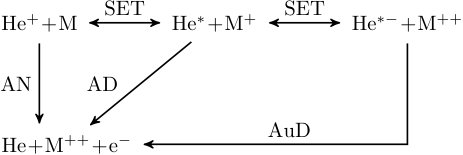 Figure 1
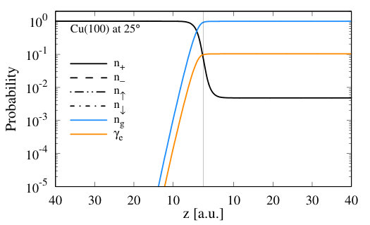 Figure 10
 Figure 10
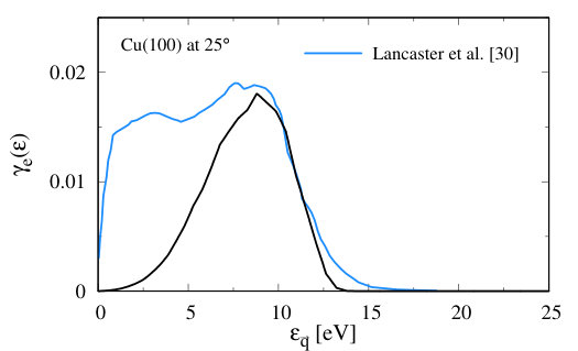 Figure 10
 Figure 10
 Figure 10
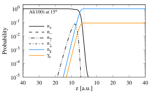 Figure 11
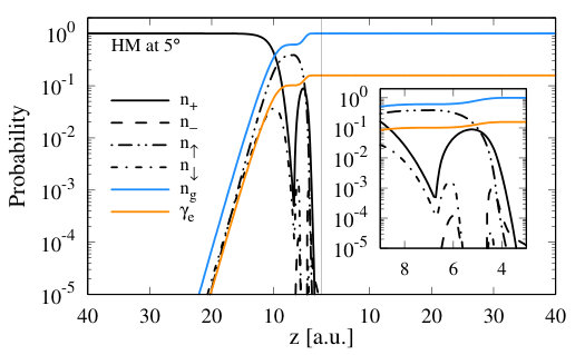 Figure 12
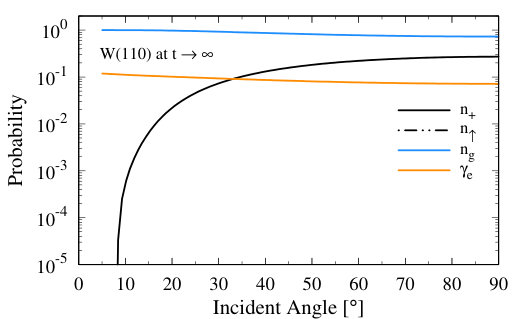 Figure 13
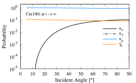 Figure 14
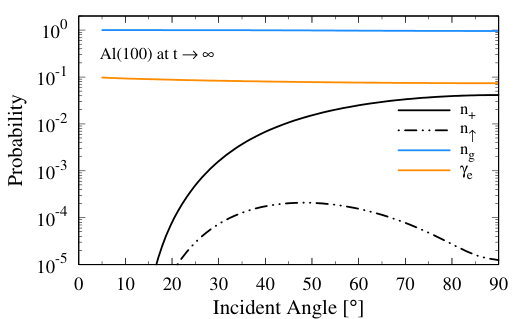 Figure 15
 Figure 16
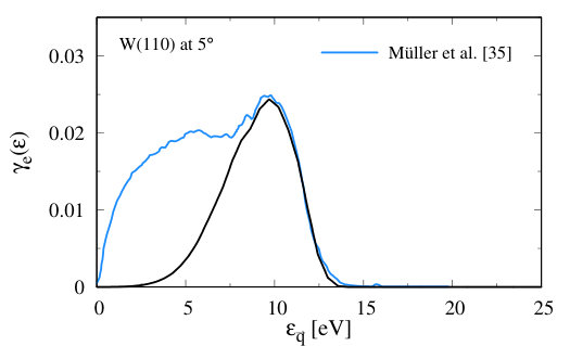 Figure 17
 Figure 18
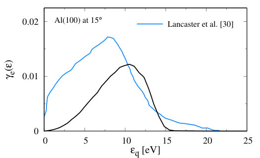 Figure 19
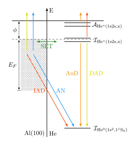 Figure 2
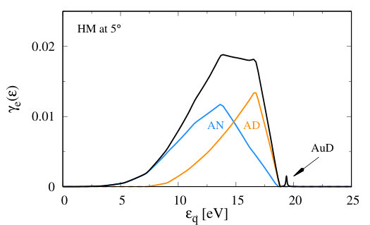 Figure 20
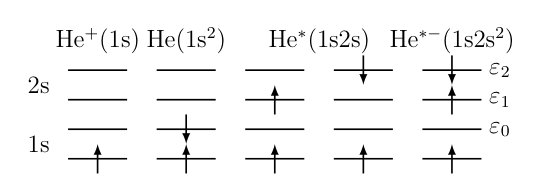 Figure 3
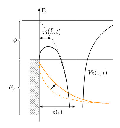 Figure 4
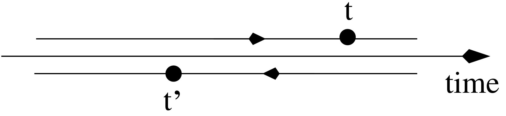 Figure 5
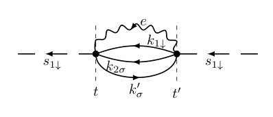 Figure 6
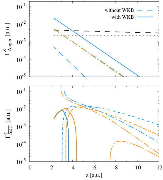 Figure 7
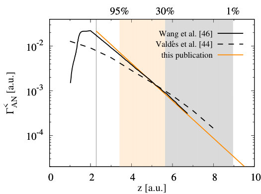 Figure 8
 Figure 8
 Figure 8
 Figure 8
 Figure 8
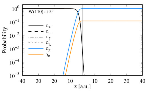 Figure 9
 Figure 9
 Figure 9
 Figure 9
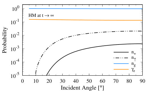 Figure 9
| [eV] | [eV] | [] | [eV] | [eV] | |||
|---|---|---|---|---|---|---|---|
| 24.5875 | – | 1.68 | – | – | – | – | |
| 4.7678 | – | 1.18 | – | – | – | – | |
| 3.9716 | – | 1.08 | – | – | – | – | |
| – | 1.25 | 0.61 | – | – | – | – | |
| – | 0.45 | 0.36 | – | – | – | – | |
| W(110) | – | – | – | 1.3 | 5.22 | 6.4 | 1.1 |
| Cu(100) | – | – | – | 1.3 | 5.1 | 7 | 1.1 |
| Al(100) | – | – | – | 1.5 | 4.25 | 11.7 | 1.1 |
| HM | – | – | – | 1.3 | 3 | 9 | 1.1 |
Peer Reviews
No public reviews on file for this paper yet. If you reviewed it on a platform where reviews are public (OpenReview, ICLR, NeurIPS, ICML), you can paste yours below so the community can read it here.
Videos
No videos yet. Explain this paper in a talk, walkthrough, or lecture? Add one.
Ion-induced secondary electron emission from metal surfaces
M. Pamperin, F. X. Bronold, and H. Fehske
Institut für Physik, Ernst-Moritz-Arndt-Universität Greifswald, 17489 Greifswald, Germany
Abstract
Using a helium ion hitting various metal surfaces as a model system, we describe a general quantum-kinetic approach for calculating ion-induced secondary electron emission spectra at impact energies where the emission is driven by the internal potential energy of the ion. It is based on an effective model of the Anderson-Newns-type for the subset of electronic states of the ion-surface system most strongly affected by the collision. Central to our approach is a pseudo-particle representation for the electronic configurations of the projectile which enables us, by combining it with two additional auxiliary bosons, to describe in a single Hamiltonian emission channels involving electronic configurations with different internal potential energies. It is thus possible to treat Auger neutralization of the ion on an equal footing with Auger de-excitation of temporarily formed radicals and/or negative ions. From the Dyson equations for the projectile propagators and an approximate evaluation of the selfenergies rate equations are obtained for the probabilities with which the projectile configurations occur and an electron is emitted in the course of the collision. Encouraging numerical results, especially for the helium-tungsten system, indicate the potential of our approach.
pacs:
34.35.+a, 79.20.Rf, 72.10.Fk
I Introduction
In low-temperature gas discharges secondary electron emission from the walls confining the plasma is an important surface collision process caused by atomic constituents of the plasma hitting the wall Lieberman and Lichtenberg (2005). Known since the early days of gaseous electronics Langmuir and Mott-Smith (1924), it moved into the focus of interest again quite recently. For instance, it has been shown that the ionization dynamics Schulze et al. (2011); Greb et al. (2013), the electron power absorption Daksha et al. (2017), and a number of other quantities and processes Hannesdottir and Gudmundsson (2016) in capacitively coupled discharges depend significantly on the secondary electron emission coefficient, that is, the probability with which an electron is released in the course of an atom-surface collision. It has been also demonstrated that the structure of the plasma sheath is strongly affected by secondary electron emission Campanell and Umansky (2016); Langendorf and Walker (2015); Sydorenko et al. (2009); Taccogna et al. (2004). The impact energies are typically in the range where electron emission is driven by the internal potential energy stored in the electronic configuration of the projectile. Auger neutralization of ions and/or Auger de-excitation of metastable species are thus the main channels of secondary electron emission A. V. Phelps and Z. Lj. Petrović (1999). Depending on the initial state of the projectile ion- and radical-induced secondary electron emission can thus be distinguished. Since the processes are also of interest for themselves as well as of importance for various kinds of surface diagnostics, for instance, secondary ion mass spectroscopy Czanderna and Hercules (1991) or metastable atom de-excitation spectroscopy Harada et al. (1997), Auger and related charge-transfer processes have been reviewed several times Monreal (2014); HP. Winter and J. Burgdörfer (2007); Winter (2002); Baragiola (1994); Los and Geerlings (1990); Brako and Newns (1989); Modinos (1987); Yoshimori and Makoshi (1986); Newns et al. (1983) since the early studies Oliphant and Moon (1930); Massey (1930); Shekhter (1937); Cobas and Lamb (1944); Hagstrum (1953, 1954) dating back to the very beginning of modern condensed matter physics. There can be thus no doubt that the basic mechanisms of secondary electron emission from surfaces have by now been identified.
Although the principles of secondary electron emission are known it is still a great challenge to measure or to calculate secondary electron emission spectra, even for free-standing surfaces not in contact with a plasma. Experimentally it requires sophisticated instrumentation Lancaster et al. (2007, 2003); Sosolik et al. (2003); Winter (2002); Hecht et al. (1998); Winter (1993); Kimmel and Cooper (1993); Müller et al. (1993); Brenten et al. (1992); Sesselmann et al. (1987); Propst (1963), whereas theoretically the challenge is to find an efficient way to deal with a many-body scattering problem giving rise to a great variety of collision pathways Bonetto et al. (2016); Iglesias-García et al. (2014, 2013); Monreal et al. (2013); Masuda et al. (2009); Valdés et al. (2005); García et al. (2003); Wang et al. (2001); van Someren et al. (2000); More et al. (1998); Lorente et al. (1998); Cazalilla et al. (1998); Lorente and Monreal (1996); Lorente et al. (1994); Marston et al. (1993); Modinos and Easa (1987). It is thus not surprising that the data base for secondary electron emission is rather sparse, especially for materials used as walls in laboratory gas discharges. There have been only a few experimental efforts devoted to measure secondary electron emission coefficients specifically for them Daksha et al. (2016); Marcak et al. (2015).
To illustrate the complexity of the physics involved we show in Fig. 1 the collision channels which may be open when a positive helium ion hits a metal surface and releases an electron. Besides Auger neutralization of the positive ion itself, there is a sequence of single-electron transfers possible, leading to neutral and negatively charged metastable states which may Auger de-excite or autodetach to the helium groundstate thereby also releasing an electron. Which one of the three channels dominates depends on the collision parameters and the metal. An unbiased description of the collision requires thus a theoretical model capable to treat all channels having a chance to be involved in the electron emission simultaneously. To present such a theory is the purpose of this work.
We do not attempt a description from first principles Iglesias-García et al. (2014, 2013); Monreal et al. (2013); Valdés et al. (2005); García et al. (2003); More et al. (1998). Instead, we use an Anderson-News-Hamiltonian for the subset of electronic degrees of freedom which are dominantly involved in the collision process. Combined with Gadzuk’s semiempirical approach Gadzuk (1967a, b) of determining the matrix elements of this Hamiltonian from classical image shifts it yields a rather flexible basis for the modeling of a great variety of projectile-target combinations. We consider this type of effective modeling, requiring at the end only a few parameters with a clear physical interpretation, particularly appropriate for describing secondary electron emission from plasma walls which are often microscopically not well characterized preventing thereby a more sophisticated modeling. Local correlations on the projectile can be taken into account by a projection operator and pseudo-particle technique pioneered by Langreth and coworkers Langreth and Nordlander (1991); Shao et al. (1994a, b). Combining this with additional auxiliary bosons to accommodate the energy defects between different electronic configurations of the projectile leads to a Hamiltonian containing as many projectile configurations as one wishes to include and at the same time is amenable to a quantum kinetic analysis Langreth and Nordlander (1991); Shao et al. (1994a, b). At the end, it leads to rate equations for the probabilities with which the electronic configurations of the projectile occur and an electron is emitted in the course of the collision. We employed this approach previously to describe electron emission from metal and dielectric surfaces due to the de-excitation of metastable nitrogen molecules Marbach et al. (2011); Marbach et al. (2012a, b) and to the neutralization of positive strontium and magnesium ions at gold surfaces Pamperin et al. (2015a, b). In this work we apply it to a positive helium ion hitting various metal surfaces. Confronted with experimental data Müller et al. (1993); Lancaster et al. (2003) the approach turns out to yield secondary electron emission coefficients of the correct order of magnitude and may even be able to produce the correct shape of the emission spectrum if it was augmented by scattering processes Lancaster et al. (2007); Brenten et al. (1992); Propst (1963) which we so far however did not include in the model.
The outline of the remainder of the paper is as follows. In the next section we set up the Anderson-Newns model for the emission channels shown in Fig. 1. Besides explaining how the matrix elements of the Hamiltonian are obtained from Gadzuk’s reasonings we also give the details of the projection operator and pseudo-particle technique which enables us to encode into a single Hamiltonian electronic configurations with different internal potential energies. Section III together with an appendix describes the quantum-kinetic derivation of the rate equations for the probabilities with which the various electronic configurations of the projectile are realized in the collision and an electron is emitted. Numerical results are presented in Sect. IV and concluding remarks summarize and assess our approach in Sect. V.
II Model
When an atomic projectile approaches a surface direct and exchange Coulomb interactions take place between their individual constituents leading to a modification of the projectile’s and target’s electronic structure. In some cases this may cause a redistribution of electrons between them accompanied perhaps by an emission of an electron. Since the projectile and the target are composite systems, to analyze these processes theoretically is a complicated many-body problem. It can be either approached with first-principle methods Iglesias-García et al. (2014, 2013); Monreal et al. (2013); Valdés et al. (2005); García et al. (2003); More et al. (1998), ideally containing the full electronic structure of the target and the projectile, or with model Hamiltonians focusing only on the subset of electronic states which are actively involved in the collision as pioneered by Gadzuk Gadzuk (1967a, b). The former is computationally very expensive. In addition it requires a rather complete characterization of the structure and chemical composition of the surface. Working atom-by-atom ab-initio methods have to know precisely which atom is sitting where. For plasma-exposed surfaces this information is not available in most cases. It is thus better not to rely on it at all and–following the second approach–to construct instead an effective Hamiltonian for that part of the electronic structure which is expected to be mostly involved in the collision process. Physical considerations may then be invoked to parameterize the model by a few quantities which are easily available and at the same time have a clear physical meaning.
The particular approach we employ is based on an Anderson-Newns-type effective Hamiltonian. Following Gadzuk Gadzuk (1967a, b) it uses classical image charges to mimic the long-range exchange interactions (polarization interactions) and a multichannel scattering theory to account in the matrix elements for single-electron transfer for the non-orthogonality of the target and projectile wavefunctions. The non-orthogonality of the wavefunctions is also an issue in the Auger channels Valdés et al. (2005). Taking it into account makes however the calculation of the Auger matrix elements even more complicated than it already is. In the model presented below we ignore therefore in the Auger matrix elements the non-orthogonality of the wavefunctions assuming implicitly that it is less important than the tunneling of the metal wavefunction through the potential barrier, arising from the overlap of the ion and surface potentials, which we take into account. The good agreement of the rate we get for Auger neutralization with the rate given by Wang and coworkers Wang et al. (2001) as well as with the rate obtained by an approach based in part on first principles Valdés et al. (2005) supports this assumption. What speaks against it is the too large ion survival probability we obtain for large angles of incidence. But the reason for this is most probably the neglect of single-electron transfer from deeper lying levels of the surface (core levels) to the shell. It is beyond the scope of the present work to include this process as well.
To furnish the formalism with wavefunctions, simple models are used for the surface potential and the electronic structure of the projectile, parameterized however such that it reproduces measured ionization energies and electron affinities. From our previous work on the de-excitation of metastable nitrogen molecules on surfaces Marbach et al. (2011); Marbach et al. (2012a, b) and the neutralization of alkaline-earth ions on gold surfaces Pamperin et al. (2015a, b) we expect this type of modeling to provide also reasonable matrix elements for the Anderson-Newns Hamiltonian describing ion-induced electron ejection from metal surfaces.
II.1 Electronic configurations and energy levels
To analyze the chain of processes outlined in Fig. 1 we consider the following electronic configurations for the He projectile: , , , and . Without loss of generality we assume the electron of the ion to have spin up. This leaves us with two non-degenerate metastable levels , a triplet and a singlet with, respectively, a spin-up and spin-down electron in the shell. The term symbols for the positive ion and the groundstate atom are and . We also consider the negative ion arising from either one of the metastable states. In both cases the term symbol is because the two electrons in the shell have antiparallel spin. It is the lowest lying negatively charged state and known to act as an intermediary in surface-induced spin-flip collisions Hemmen and Conrad (1991); Borisov et al. (1995). It may thus also play a role in secondary electron emission. In principle there are of course additional configurations possible. For instance, the metastable state could be also involved. We expect it however to be less important for the collision we consider because orbitals lead to smaller matrix elements and thus to smaller transition rates.
Far away from the surface the projectile configurations are characterized by a discrete set of energies representing the ionization energies or electron affinities depending on whether the configurations are electrically neutral, positive, or negative. For the reaction scheme shown in Fig. 1 we need the single-electron ionization energies , , and , that is, the thresholds of the first ionization continua of the helium configurations given in the subscripts, as well as the single-electron affinities and , where the subscripts indicate again the configurations the energies belong to. How these (positive) energies relate to the vacuum level is shown in Fig. 2 together with the processes they are involved in. While the projectile approaches the surface the energy levels shift. Assuming a polarization-induced image charge interaction to be responsible for the shifts, the ionization levels move upward in energy whereas affinity levels move downwards Newns et al. (1983). Close to the surface short-range interactions may modify the shifts More et al. (1998). The processes we are interested in occur however sufficiently far away from the surface that short-range interactions are not yet important. To take all this into account, we define five time-dependent single-electron energy levels,
[TABLE]
with the subscript indicating the shell and the spin of the electron and the time-dependence arising from the collision trajectory,
[TABLE]
where is the projectile’s velocity component perpendicular to the surface and is the turning point of the trajectory. The energy levels (1)–(5) are thus time-dependent ionization energies and electron affinities. Note, describes the classical center-of-mass motion of the projectile resulting from the trajectory approximation Modinos (1987) being justified because of the large mass of the projectile. The turning point is usually a few Bohr radii before the crystallographic ending of the surface. It arises from short-range repulsive forces. Our choice for , which in general depends on the projectile and the target, is guided by the calculations of Lancaster and coworkers Lancaster et al. (2003) showing that the neutralization of ions at impact energies , which is also the upper limit in the gracing incident experiments we compare our results with, takes typically place in front of the surface where denotes the Bohr radius. We can thus choose , as suggested by Modinos and Easa Modinos and Easa (1987), without affecting the charge-transfer too much. Indeed our final results are rather robust against changes in up to . The position of the image plane , appearing in (1)–(5), is used as a fitting parameter but it should be around Lang and Kohn (1970).
In addition to the energy levels of the projectile we also need the energy of an electron in the conduction band of the metal and the energy of an unbound electron at position in front of the surface. Modeling, as in our previous work Marbach et al. (2011); Marbach et al. (2012a, b); Pamperin et al. (2015a, b), the metal by a three-dimensional step potential,
[TABLE]
with depth , where is the Fermi energy of the metal and the work function,
[TABLE]
with the effective mass of an electron in the conduction band of the metal. Assuming moreover a plane wave for the wavefunction of an unbound electron in front of the surface, its energy is given by
[TABLE]
where the second term takes the interaction of the electron with its image into account.
Since by assumption the shell is always occupied by a spin-up electron, we in effect model the projectile by a three-level system with energies , , and as illustrated in Fig. 3. An important feature of the model is that the energies depend on the occupancy of the levels and–in the case of the negative ion configurations–on the way the occupancy was build-up. To take this into account we employ operators
[TABLE]
projecting onto states of the three-level system containing electrons in the energy levels . Defining
[TABLE]
with projections to the remaining states required for the completeness
[TABLE]
to be zero, it is possible to adjust , , and to the internal energetics of the projectile configurations involved in the atom-surface collision we want to model. The operator defined in (16) will be also required in the quantum kinetic approach described in the section III.
II.2 Wave functions and matrix elements
To set up the Anderson-Newns Hamiltonian for the charge-transferring atom-surface collision processes we are interested in we require a series of matrix elements. Their calculation is based on a particular choice of wavefunctions which we now describe.
As in our previous work Pamperin et al. (2015a), the electronic states of the metal are the wavefunctions of the step potential (7). For they describe bound electrons whereas for they contain a transmitted and a reflected wave. From the work of Kürpick and Thumm Kürpick and Thumm (1996) we expect little changes had we used other wavefunctions for the surface based, for instance, on the Jenning-Jones-Weinert potential Jennings et al. (1988) instead of the potential step. For the states of the projectile’s and shell we take hydrogen wavefunctions and with effective charges adjusted to reproduce the ionization energies and electron affinities, , , , , and . For the shell the modified hydrogen wavefunction is in excellent agreement with the Roothaan-Hartree-Fock wavefunction for the helium groundstate given by Clementi and Roetti Clementi and Roetti (1974). To estimate the quality of the wavefunction for the shell we compared it–due to lack of Roothaan-Hartree-Fock calculations for excited helium states–with the Roothaan-Hartree-Fock wavefunction of the lithium groundstate Clementi and Roetti (1974). As expected, the agreement is not as good as for the shell. Since however we found for the metals we investigated charge-transfer to be dominated by Auger neutralization, which involves only the shell, we did not attempt to improve the wavefunction for the shell. The projectile’s continuum states are–as mentioned above–approximated by plane waves . Thereby we ignore distortions of the wavefunctions due to the core potential of the projectile, turning plane waves into Coulomb waves. It is only an issue for Auger de-excitation and autodetachment, which we found however not to be the dominate scattering channels. We did therefore not include this complication.
Having wavefunctions we can construct matrix elements for the processes shown in Fig. 2. Denoting the position of the projectile by with defined in (6) and following Gadzuk Gadzuk (1967a, b) as well as our earlier work Marbach et al. (2012a); Pamperin et al. (2015a, b) we obtain
[TABLE]
for the matrix element controlling single-electron transfer between the conduction band of the surface and the ionization/affinity levels of the projectile originating from its shell,
[TABLE]
for the matrix element driving Auger neutralization into the groundstate, that is, the shell of the projectile, and
[TABLE]
for the direct and indirect Auger de-excitation, respectively, involving the projectile’s and shells. Finally, the matrix element for autodetachment reads
[TABLE]
In contrast to the other matrix elements it is, within our modeling, independent of time (that is, independent of the distance ) since it describes a local interaction acting at the instantaneous position of the projectile.
Although the assumptions about the wavefunctions used in (17)–(21) are strong, we stick to it because they allow us to pursue the calculation of the matrix elements to a large extent analytically by means of lateral Fourier transformation, which in turn substantially reduces the numerical effort (which is still large) when it comes to the solution of the kinetic equations. To estimate the validity of our approach, we compare our results with experimental data. As we will see the agreement is sufficiently good to suggest that the approximate matrix elements we use are not too far away from the exact matrix elements which we however do not know. Our matrix elements contain a number of parameters which we list in Table 1. As indicated in the caption of the table we use parameters from different sources. If the parameters were given directly for the experiments we compare our data with, we took these values. This was the case for the work functions of copper and aluminum and for the affinity levels. The rest of the parameters we collected from data tables. The effective charge and the position of the image plane were determined as stated above.
An important additional aspect affecting Auger neutralization and indirect Auger de-excitation into the projectile groundstate is the enhancement of the wavefunction of the surface electron which fills the hole in the shell of the projectile. It arises from the modification of the step potential mimicking the surface by the Coulomb potentials of the ion and its image and the image potential of the electron. In effect, the step potential (7) becomes a potential barrier,
[TABLE]
with
[TABLE]
as shown in Fig. 4, through which the surface electron can tunnel. Following Propst Propst (1963) and Penn and Apell Penn and Apell (1990), we take this into account by a semiclassical correction to the electron’s wavefunction using the WKB approximation. The dependence of the wavefunction of a metal electron with is given by
[TABLE]
For the step potential,
[TABLE]
with . Using the WKB method to account for the tunneling of the electron through the barrier (see Fig. 4),
[TABLE]
with and and the turning points of the under-the-barrier motion of the electron. Neglecting in (23) the image potential of the metal electron, that is, the third term, can be determined analytically leading to the black dashed line in Fig. 4. By numerical integration we then find the adjustment ratio,
[TABLE]
which depends only weakly on . Hence, by replacing in Eq. (25) by
[TABLE]
we approximately take into account the tunneling-induced enhancement of the metal electron wavefunction at the projectile position as illustrated in Fig. 4. The assumptions made in the calculation of (27) hold as long as is below the Fermi energy . This is, however, the case since the electron filling the shell in an Auger process originates from an occupied state of the conduction band of the surface. In Section IV we will see that the WKB correction brings the transition rate for Auger neutralization we obtain in very good agreement with the rate given by Wang and coworkers Wang et al. (2001). It is based on the work of Lorente and Monreal Lorente and Monreal (1996) and has been also used by others Lancaster et al. (2003); More et al. (1998). For the distances we are interested in it is moreover in reasonable agreement with calculations based in-part on first principles Valdés et al. (2005).
II.3 Hamiltonian
We now have everything needed to begin the construction of the Hamiltonian for the processes outlined in Fig. 1. With the energy shifts and matrix elements given above it reads
[TABLE]
where the fermionic operators annihilate (create) an electron in the level with the spin as indicated in Fig. 3. Likewise the fermionic operators and annihilate (create), respectively, an electron with spin in the conduction band of the target surface or the continuum of the projectile. The projection operators as defined in (10) guarantee that each individual term is projected onto that subspace of the three level system representing its physical domain of applicability. For instance, the term describing Auger neutralization (fifth last term) must contain a factor because it involves only the positive ion and the groundstate, that is, in the notation of the three-level system, the states and .
An essential aspect of our approach is that it allows to treat electronic configurations of the projectile with defects in their internal energies. More specifically, the numerical value of the energy level depends on the occupancy of the three-level system. In case and are occupied, denotes an affinity levels of either or whereas in the case is empty stands for the ionization level of either or . To switch between ionization and affinity levels we introduce two auxiliary bosons and with energy
[TABLE]
where labels the complementary spin orientation of the electron in the shell of the two configurations between the boson is expected to switch. With this trick Marbach et al. (2012b) all processes encoded in the Hamiltonian conserve energy irrespective of whether a negative ion or a metastable configuration is involved.
The Hamiltonian (II.3) is rather involved but the physical meaning of the various terms is almost selfexplaining. For instance, the first term describes the ionization and affinity levels of the projectile while the next three denote the auxiliary bosons, the continuum of surface states, and the continuum of the projectile. The following four terms are the single-electron transfers into and out of the metastable ionization and affinity levels. Auger neutralization of the positive ion, direct Auger de-excitation of the metastable singlet configuration, indirect Auger de-excitation of the metastable triplet and singlet configurations, and the autodetachment of the negative ion are given by the last five terms. Note, due to the Pauli principle direct Auger de-excitation is only possible for the singlet metastable state (see Fig. 3 and Fig. 2). Hence, it affects only the levels and . Indirect Auger de-excitation, in contrast, is not restricted in such a way.
Working directly with the Hamiltonian (II.3) is cumbersome because it is not suited for a diagrammatic analysis which on the other hand is a powerful tool to derive kinetic equations as shown by Langreth and coworkers Langreth and Nordlander (1991); Shao et al. (1994a, b). We rewrite therefore the states making up the projection operators in terms of pseudo-particle operators , and defined by
[TABLE]
Hence, , , , , and create, respectively, the positive ion, the negative ion, the groundstate, the triplet metastable state, and the singlet metastable state. The statistics of the operators is fixed by the Fermi statistics of the operators and physical considerations Marbach et al. (2012b). Since the positive and negative ion represented, respectively, by and contain an odd number of electrons, because of the spin-up electron always present in the shell, but not explicitly included in the three level system (see Fig. 3), the operators and should be endorsed with Fermi statistics. The groundstate and the metastable configurations, , , and , on the other hand, carry an even number of electrons. Hence, it is natural to endorse the operators , , and with Bose statistics.
The relation between the operators , , and , which are single-electron operators, and the pseudo-particle operators defined in (II.3), which create many-electron states, that is, whole electronic configurations, is found by letting the former act on the completeness relation (16). The result is
[TABLE]
where the minus signs guarantee the fulfilment of the anti-commutation relations. Inserting (II.3)-(II.3) into (II.3), carrying out all projections, and making at the end replacements of the sort we finally obtain the Anderson-Newns Hamiltonian in pseudo-particle representation:
[TABLE]
The physical meaning of the various terms of the Hamiltonian is now particularly transparent. Consider, for instance, the fourth last term. It describes Auger neutralization (and its reverse which has to be included to make the Hamiltonian Hermitian) and hence the creation/annihilation of the projectile groundstate and a secondary electron by simultaneously annihilating/creating a positive ion and two metal electrons. Likewise the last term describes autodetachment (and its reverse), that is, the creation/annihilation of the groundstate by annihilation/creation of the negative ion due to creating/annihilating an electron in the continuum of the projectile. In the next section we will use this Hamiltonian to determine the probabilities with which the various projectile configurations appear and an electron is emitted in the course of the atom-surface collision.
III Quantum kinetics
With the electronic configurations of the He projectile encoded in an effective three-level system holding either none, one, or two electrons with the spin polarizations given in Fig. 3 we can now calculate the probability with which an electron is emitted via Auger neutralization or the sequence of single-electron transfers leading to Auger de-excitation or autodetachment as shown in Fig. 1. For that purpose we use the quantum-kinetic method which rests in our case on the contour-ordered Green functions Kadanoff and Baym (1962); Keldysh (1965),
[TABLE]
where the time variables run over the Keldysh contour shown in Fig. 5. The first four functions describe the positive ion, the groundstate, the two metastable states, and the negative ion while the last three apply, respectively, to an unbound electron in the projectile’s continuum, the electrons in the conduction band of the target surface, and the auxiliary bosons. The operators making up the Green functions evolve in time with the full Hamiltonian (II.3) and the brackets denote the statistical average with respect to the initial density matrix describing one-auxiliary-boson states, surface electrons in thermal equilibrium, and an empty projectile, that is, a positive ion.
Following the work of Langreth and coworkers Langreth and Nordlander (1991); Shao et al. (1994a, b) we use Dyson equations for these functions to derive a set of equations for the occurrence probabilities/occupancies of the bound projectile states, that is, the affinity and ionization levels. Introducing the selfenergies , , , and for the Green functions , , , and , we obtain ( in this section and the two appendices)
[TABLE]
for the time evolution of the probabilities , , , and with which, respectively, the positive ion, the groundstate, the two metastable states ( denoting the triplet and the singlet), and the negative ion occur.
Equation (III)–(III) are exact but of course not closed in terms of the occurrence probabilities. To proceed we set up the selfenergies in the non-crossing approximation, utilize that the matrix elements (17)–(21) factorize approximately in functions of and the set of vectors, and finally apply the semiclassical approximation to (III)–(III) developed by Langreth and coworkers Langreth and Nordlander (1991); Shao et al. (1994a, b) which in essence is a saddle-point integration in time.
In order to get an impression about how the selfenergies look like, we show in Fig. 6 the contribution to the selfenergy , entering the Dyson equation of the groundstate propagator , which arises from the Auger neutralization. There are also contributions to due to direct and indirect Auger de-excitation as well as autodetachment. They are given in Appendix A together with the other selfenergies entering Eqs. (III)–(III) and some details concerning their calculation. Using standard diagrammatic rules Lifshitz and Pitaevskii (1981) the diagram shown in Fig. 6 translates to
[TABLE]
The time variables run over the (Keldysh) contour, that is, from to and back as shown in Fig. 5. Application of the Langreth-Wilkins rules Langreth and Wilkins (1972) with a subsequent projection to the subspace encoded in the completeness relation (16) yields the analytic pieces of the selfenergies, where the time variables are now taken from the real-time axis,
[TABLE]
with the superscripts , and indicating the less-than, greater-than, and retarded pieces of the selfenergy (50). In accordance with the non-crossing approximation the surface electrons are propagated by the undressed Green function,
[TABLE]
Only the propagators applying to the ionization and affinity levels of the projectile, , , , and are modified by selfenergies.
Due to the approximate factorization of the time and momentum dependencies of the matrix elements it is possible to express the selfenergies by functions arising from the application of the golden rule to the respective interaction terms in the Hamiltonian. The physical meaning of the functions is the one of a (partial) levelwidth. Since they eventually determine the rates entering the rate equations for the occurrence probabilities given below, we list the functions, however, without derivation which is quite lengthy. An exemplary calculation is presented in Appendix B.
Single-electron processes are characterized by
[TABLE]
while Auger processes are encoded in
[TABLE]
with
[TABLE]
where on the rhs of the last equation or depending on whether the negative ion is formed out of or . Notice, in contrast to the other levelwidth functions, does not depend on time since the matrix element is independent of time and the time dependencies of the energies in the delta function contained in cancel.
To get the expressions we used the arguments Langreth and Nordlander Langreth and Nordlander (1991) developed for simplifying selfenergies due to single-electron transfer with the exception that in the levelwidths arising from Auger and autodetachment processes the distribution functions for the surface and continuum electrons, and , are not separated out from the summations in momentum space. The functions and encode, respectively, initially occupied and empty states of the conduction band of the metal. Hence, is the Fermi-Dirac distribution function at temperature of the surface. The distribution function for an electron in the continuum of the projectile for and equal to zero otherwise.
The saddle-point integration in time utilizes the fact that the Green functions lead to selfenergies which are strongly peaked at equal times. In effect, the time variables of the projectile Green functions (including the ones entering the selfenergies) on the rhs of Eqs. (III)–(III) are set to equal times once the time integrations are carried out. Identifying less-than functions at equal times with occurrence probabilities/occupancies and realizing that retarded functions at equal times are simply equal to unity in the time intervals where they do not vanish, we obtain the rate equations
[TABLE]
which are, due to the completeness (16), subject to the constraint
[TABLE]
The compliance of (65) can be easily verified by noting
[TABLE]
and summing each column of (64) which results in the nullifying of the rates. Thus, the constraint (65) is fulfilled. Also note, with respect to the diagonal of the coefficient matrix in (64), the entries in the lower triangle comprise only less-than rates whereas in the upper triangle only greater-than rates appear. Besides having no entries of greater Auger rates , , , , and the matrix is symmetric.
For the interpretation and numerical solution of (64) we apply to the rates the adiabatic approximation. The rates in (64) can then be expressed by the levelwidth functions. For the single-electron transfers the adiabatic approximation yields Langreth and Nordlander (1991)
[TABLE]
with and defined in (54) and (55), respectively. The Auger and autodetachment transition rates reduce in the adiabatic approximation simply to the levelwidths functions given in Eqs. (56)–(59). Hence,
[TABLE]
At this point one clearly sees that in the derivation of the levelwidths due to Auger and autodetachment processes we did not factorize out the distribution functions as it is the case in the derivation of the levelwidths due to single-electron transfers. As a result, the distribution functions for the metal electron appear in front of the width functions in (67) and (68) but not in (69)–(72), where they are contained in the width functions themselves.
A particular characteristic of the adiabatic rates, in contrast to the quantum-kinetic rates coming out directly from the saddle-point approximation to (III)–(III) as discussed in Appendix A, is that they are positive semidefinite. With the adiabatic rates Eq. (64) can thus be interpreted straightforwardly: The lower triangle describes the gain of the projectile configurations by the processes entering this part of the matrix. In terms of Fig. 1 the lower triangle encodes the transitions from left to right and from top to bottom, starting with the positive ion which is the initial configuration. The diagonal of the matrix gives the losses of the configurations. In contrast to the lower triangle, the upper triangle describes indirect gains for the configurations. It encodes the transitions in Fig. 1 from right to left. Moving from bottom to top is not allowed energetically. In case it was, the last column of the matrix would be filled with greater-than Auger rates.
With the rate equation (64) it is now particularly easy to write down a differential equation for the probability of emitting a secondary electron. Every process outlined in Fig. 1 that leads to the occurrence of the ground state generates an excited electron (see Fig. 2). Thus, the rate equation for the probability to emit a secondary electron at time with energy is,
[TABLE]
It has the same structure as the rate equation for the groundstate. The spectrally resolved rates entering this equation are essentially the ones given in (69)–(72) except that the integration over the magnitude of the wave vector of the excited electron is not carried out and that the conditions for escaping from the surface have to be taken into account Baragiola (1994). The reason is the following: An excited electron becomes a secondary electron only if it is also able to escape from the location where it is generated. If it is created on-site the projectile due to autodetachment or indirect Auger de-excitation the electron has to overcome its image potential requiring, in the spirit of the escape cone model Feuerbacher and Wallis (1976), and
[TABLE]
where is the angle between and the outward surface normal. The -integration in is thus cropped leading to modified rates which we denote in (III) by . In case, the electron is generated inside the solid surface, that is, by Auger neutralization or direct Auger de-excitation, the escape of the electron is also affected by scattering processes. Assuming elastic scattering to be most important, the electron arrives isotropically at the interface leading to the rates with
[TABLE]
the surface transmission function Baragiola (1994).
Solving (III), the energy spectrum of the emitted secondary electron is obtained by
[TABLE]
and the probability that an electron gets emitted at all, that is, the secondary electron emission coefficient (coefficient) follows by integration over all energies,
[TABLE]
In order to compare our results with experiments we apply one more modification. Surface scattering experiments typically occur under conditions of grazing incidence Winter (2002); Müller et al. (1993). The lateral velocity of the projectile is thus very large. To account in our calculations for the smearing of the metal electron’s Fermi-Dirac distribution induced by the lateral motion of the projectile, in addition to the thermal smearing of the distribution function due to the surface temperature , we replaced for the numerical calculations in the formulas given above the function by an angle-averaged velocity-shifted distribution Sosolik et al. (2003),
[TABLE]
with the work function of the surface, , and , where is the surface’s Fermi wave number. From the projectile’s perspective the velocity smearing populates surface states above the Fermi energy thereby potentially strengthening charge-transfer processes from the metal to the He metastable states which, due to image shifting, turn out to be well above the Fermi energy.
Let us finally say a few words about the numerics we applied. The calculation of the levelwidths (54)–(59) requires at least a two dimensional integration over the solid angle of or and at worst, in the case of Auger neutralization, an integration in nine dimensions. In the case of indirect Auger de-excitation, an additional 6-dimensional numerical integration must be performed over and , since the method of lateral Fourier transformation, unlike for the other channels, does not lead to an analytic result. The integrations are done by a MPI parallelized Monte Carlo Vegas code Lepage (1978) for a discrete number of different times. To obtain the matrix elements at times in between we utilized multidimensional-linear interpolation. The same strategy was used for the additional integrals of the indirect Auger de-excitation. Because of the multidimensionality, using more advanced interpolation methods, e.g. splines, would be a difficult undertaking, not necessarily leading to better results. In addition, an interpolation of the time-arguments of the rates (67)–(71) is necessary to solve the rate equation (64). Here, when interpolating, we take advantage of the fact that the rates are almost exponential, which greatly improves the results. To solve the rate equation (64), finally, we employed the explicit embedded Runge-Kutta Cash-Karp method also provided by the GNU scientific library. We have put importance on a reasonable error propagation resulting in a relative numerical error of the calculated occurrence/occupation probabilities of less than .
IV Results
In this section we present numerical results calculated for the material parameters listed in Table 1. We use atomic units measuring length in Bohr radii and energy in Hartrees. The surface is assumed to be at room temperature leading to a thermal broadening of the Fermi-Dirac distribution which is much less than the velocity-induced smearing. In the calculations we used therefore (78) in the limit .
We start the discussion with Fig. 7, where we plot the transition rates entering the rate equation (64) for a ion hitting an aluminum surface with and angle of incidence . The upper panel shows the Auger rates whereas the rates due to single-electron transfer are shown in the lower panel. To demonstrate the importance of the WKB correction to the Auger rates we plot in the upper panel calculated with and without it. Clearly, the WKB correction to the metal wavefunction has a dramatic effect. It increases by two orders of magnitude. A comparison with the results from other groups, discussed in the next paragraph, indicates that the WKB correction is essential for producing the correct order of magnitude. The WKB correction is also important for indirect Auger de-excitation. Due to lack of data we can however not compare it with other results. Before discussing the reliability of the rates, a few general remarks are in order. The rates for indirect Auger de-excitation and Auger neutralization decrease with distance whereas the rate for direct Auger de-excitation remains almost constant. This is simply because it is a transition between two ionization levels which shift more or less identically. In this respect it resembles the rate for autodetachment which is exactly a constant within our modeling and moreover independent of the target surface. Comparing the Auger rates with the rates for single-electron transfer (plotted in the lower panel) shows that Auger rates are in general smaller implying that the latter dominate the former in situations where both are possible. The spin-dependence of the rates arises primarily from the energy difference of the singlet and triplet ionization/affinity levels. The closer the levels to the vacuum level the more extended is the wavefunction of the surface electron taking part in the process leading to a larger matrix element and hence transition rate. For the same reason decreases near the turning point.
To estimate the quality of our WKB-modified rate for Auger neutralization we compare it in Fig. 8 with the rate given by Wang and coworkers Wang et al. (2001). It is essentially an extension of the Auger neutralization rate worked out by Lorente and Monreal Lorente and Monreal (1996) to distances and well established Lancaster et al. (2003); More et al. (1998). The agreement for is almost perfect, although the two rates are obtained by different methods. Additional support for our rate (and hence also for the one of Wang and coworkers) stems from the comparison with the rate obtained by Valdés and coworkers Valdés et al. (2005) using an approach based in part on first principles. At distances, where Auger neutralization is expected to take place, there is an astonishingly good agreement between the three rates indicating that the three approaches contain the essential physics operating at these distance. They differ hence only in aspects becoming important at high impact energies, when the projectile gets closer to the target or may even penetrate it, as can be seen by the deviations at short distances. Since the model assumptions are the same for the other rates we calculate, we except them to be also of the correct order of magnitude for , that is, at distances where at moderate impact energies charge-transfer takes place.
Having calculated the transition rates we can solve the rate equation for the instantaneous occurrence probabilities , , and , applying respectively to the positive ion, the triplet and singlet metastable state, the negative ion, and the groundstate. Figure 9 shows results for these quantities for a ion hitting different surfaces at different angles of incident and different kinetic energies. The abscissas show the separation of the projectile from the surface. Starting on the left at a distance it moves along the incoming branch of the trajectory towards the turning point , indicated by the thin vertical line, where it is specularly reflected to move back to the distance along the outgoing branch of the trajectory shown on the right. The kinetic energy of the projectile was set to eV [W(110)], eV [Cu(100)], and eV [Al(100)] which are the kinetic energies at which the electron emission spectra have been determined experimentally for these metals Müller et al. (1993); Lancaster et al. (2003). Below we will compare the calculated spectra with the experimentally measured ones. We also studied a hypothetical metal, termed ”HM”, with and to make all processes outlined in Fig. 1 to work in concert for an ion with and .
In case of tungsten and copper, the work functions, (tungsten) and (copper), are too large to enable resonant single-electron transfer into the metastable states and . Hence, at the end only the groundstate becomes occupied via Auger neutralization, with probability unity for tungsten and near unity for copper. The ion is thus very efficiently neutralized at both surfaces. For copper however the positive ion has a slim chance to survive. Its occurrence probability at the end of the collision . The secondary electron emission probability, the coefficient, is for both cases around . Analyzing the two cases a bit deeper one realizes that the larger angle of incident makes the projectile hit the copper surface with a much larger perpendicular kinetic energy. Since the major part of the reaction still takes place for distances , the interaction time for copper is much shorter than for tungsten. This may be the reason for the ion to survive the collision, albeit only with a very small probability.
For an aluminum surface, the work function is low enough to allow on the incoming branch of the trajectory also the formation of the configuration. Its occurrence probability raises to sizeable values around (double-dot dashed line in the lower left panel of Fig. 9). Secondary electron emission due to indirect Auger de-excitation it enables is however very weak. We find only one percent of the total emission probability to be due to this process, consistent with the statement of Wang and coworkers Wang et al. (2001) that it is negligible. As can be seen in the lower left panel of Fig. 9, secondary electron emission due to indirect Auger de-excitation becomes small compared to emission due to Auger neutralization because its starting point, the metastable states, are most of the time much less probable than the positive ion, the starting point for Auger neutralization. Hence, although the rates for indirect Auger de-excitation and Auger neutralization are of the same order of magnitude, differing only by a factor two (see Fig. 7), the efficiency of the two processes is very different due to the collision dynamics. Iglesias–García and coworkers Iglesias-García et al. (2014), in contrast, report on the importance of single-electron transfer, and hence the formation of metastable states, for the neutralization of a helium ion at an aluminum surface. The noticeable temporary occurrence probability we find for seems to support their view. However, its role for the outcome of the collision process is very sensitive to the position of the Fermi energy and the shift of the ionization level encoded in Eq. (5). In our case, we find that at the end plays a subdominant role. Further investigations are required to clarify the issue, taking improved models for the electronic structure of the surface and the polarization-induced level shifts into account.
The situation we termed ”HM” was constructed to demonstrate the interplay of all channels outlined in Fig. 1. For this case, the instantaneous occupancies shown in the lower right panel of Fig. 9 and its inset are more involved. During the approach of the projectile to the surface both metastable states– and –become occupied, enabling thereby direct (from the singlet configuration) and indirect (from the singlet and triplet configurations) Auger de-excitation, in addition to Auger neutralization. The occurrence probability of the positive ion drops accordingly. At before the turning point reaches a local minimum but starts to rise again for a brief amount of time before it drops to very small values. At the same time the probability for decreases after reaching its maximum. Having only an ionization energy of around , the drop is due to the image-shift encoded in (2) which pushes the ionization level above the Fermi energy thereby turning the weak gain due to single-electron transfer off and the strong electron loss due to the process on. In addition, there is a strong loss due to direct Auger de-excitation. The triplet configuration is affected similarly, albeit at a later time due to the greater ionization energy and the lacking of the strong direct Auger de-excitation (which is absent because of the Pauli principle). When the electron transfers from the metastable states back to the surface via single-electron transfer the positive ion is restored. Hence, the occurrence probability for the positive ion rises again near the surface, allowing for a revival of the Auger neutralization. As a result, the occurrence probability jumps close to the surface to near unity. With the ionization levels shift of course also the affinity levels. If they approach the Fermi energy from above, a negative ion becomes possible. Hence, for a very short time interval, when the occurrence probabilities for the two metastable configurations are already decreasing, a negative ion is formed. It decays however nearly instantly because of single-electron transfer and autodetachment.
In all four cases depicted in Fig. 9, the outgoing branch lacks complex behavior. For the chosen angles of incident and kinetic energies the groundstate is always formed very efficiently along the incoming branch. Since the groundstate is not subject to a loss channel, it cannot be destroyed. The constraint (65), which has to be satisfied at any instant of time, ensures then that the other configurations vanish as soon as the groundstate appears with probability near unity. At the end of the collision the groundstate configuration dominates. Only for copper we find a noticeable probability for detecting at the end also a positive ion. Although the other configurations have vanishingly small probabilities at the end they may nevertheless affect the outcome of the collision because of their presence at intermediate times.
Experimentally accessible are only the probabilities at the end of the collision. Let us thus investigate their dependence on impact energy and angle of incidence. Figure 10 shows for the same impact energies as in Fig. 9 the angle dependence of the probabilities for detecting at the end of the collision the configurations included into our modeling as well as for emitting an electron. The results for tungsten and copper are again very similar. At small angles essentially only the groundstate is formed, because Auger neutralization is the dominant process. As the angle increases the kinetic energy perpendicular to the surface also increases, lowering thereby for all channels the interaction time. This leads to a steady increase of the occurrence probability for the positive ion although it remains for all angles much smaller than the probability for the groundstate. The ion survival probability is largest for perpendicular incidence, which is also most relevant for plasma applications. For tungsten we obtain around , which is two orders of magnitude too large compared to the experimental data Hagstrum Hagstrum (1961) found long time ago. But survival probabilities on the order of are typical (see for, instance, Fig. 26 in Ref. Monreal (2014)). Moving the turning point closer to the surface reduces the survival probability but not by two orders of magnitude. It is not possible to push this number to the correct order of magnitude by simply adjusting model parameters. We expect the neglect of single-electron transfer to the shell to be responsible for the too large survival probability at perpendicular incidence. The impact energy of the projectile is in this case the highest leading to the closest encounter with the surface where single-electron transfer from core levels may already become important. To include it is however beyond the scope of the present work. In addition non-orthogonality corrections to the Auger rates may become also an issue for perpendicular incidence.
The final probabilities for aluminum and the hypothetical metal, shown in the lower two panels, behave also similarly. The main difference to tungsten and copper is the formation of the metastable triplet state . It forms on the incoming branch of the trajectory because the lowering of the work function enables single-electron transfer into the metastable state and the shortening of the interaction time reduces the electron transfer back to the metal which, in effect, leads to a freezing-in of the metastable state. For the hypothetical case the occurrence probability for the metastable triplet state is even larger than the one for the positive ion indicating that at intermediate times the singlet metastable state as well as the negative ion state may have also played an active role in the collision.
We now turn to the energy spectrum of the emitted electron. In Fig. 11 we present results based on Eqs. (III) and (76) together with experimental data for tungsten from Müller and coworkers Müller et al. (1993) and copper and aluminum from Lancaster and coworkers Lancaster et al. (2003). Only the former group gives also an estimate for the total emission probability, that is, the coefficient. As far as the data for tungsten are concerned we can thus compare absolute numbers. For copper and aluminum this is not possible since no value for the coefficient was given by the experimentalists. In addition, the area embraced by the measured emission spectra, which would give the emission coefficient according to (77), cannot be used either because the experimental data are presented in arbitrary units.
Müller and coworkers estimate for a ion hitting a tungsten surface with eV and . We weighted their emission spectrum according to (77) to match this number. A comparison of the weighted experimental spectrum with our data is shown in Fig. 11. The agreement is quite satisfying, in particular, as far as the high-energy side of the spectrum is concerned. The high-energy cut-off and the maximum of the emission spectrum match quite well indicating that our approach may be able to estimate at least the order of magnitude of secondary electron emission in cases where no experimental data are available. At low energies experimental and theoretical data deviate. The theoretical secondary electron emission coefficient is thus roughly only one-half of the experimental estimate. The reason is the following: We did not include processes relaxing the energy of the excited electron. Scattering cascades Propst (1963); Lancaster et al. (2007) and higher order Auger processes Brenten et al. (1992) involving more than two electrons are often attributed for this. Since the physical origin is not yet quite clear, we did not consider it for the purpose of this work. Our energy spectrum for the secondary electron leaving the tungsten surface is entirely due to Auger neutralization; the other channels of Fig.1 are energetically closed. Without scattering cascades and higher-order Auger processes included, it applies only to the high-energy side of the spectrum. There, however, the agreement is rather good.
The good match of the theoretical and experimental emission spectra for tungsten at high energies suggests a way to scale the data of Lancaster and coworkers such that they can be compared to the calculated spectra. An important consequence of the scaling is that we can then also estimate the coefficients for copper and aluminum. The ratio of the theoretical and experimental secondary electron emission coefficients for tungsten is roughly one-half because of the neglect of scattering cascades and higher-order Auger processes. Assuming that both types of processes are essentially the same for the metals under discussion, we scale the emission spectra of Lancaster and coworker also in this manner. Hence, we set where is the ratio obtained from the tungsten data. The scaling provides an absolute scale to the experimental data and hence also the -coefficients.
As can be seen from Fig. 11, applying the scaling to the data for copper leads at high energies again to a good agreement between the experimental and the theoretical emission spectra. As for tungsten, the high-energy side of the spectrum is determined largely by Auger neutralization. From the calculation we obtain for copper producing . For aluminum the matching of the high energy tails is not as good. The small work function and the large Fermi energy lead in this case to a broad spectrum for the electron emitted by Auger neutralization. In addition, the low work function enables indirect Auger de-excitation although it provides only a small amount of secondary electrons between and . For aluminum our approach yields , a bit lower than for tungsten and copper. The estimate for the experimental value is thus . For aluminum the theoretically obtained emission spectrum does not even match the measured data at high energies. In the case of tungsten and copper the processes leading to electron emission at lower energies are well separated from electron emission due to Auger neutralization. The latter leading to a maximum at the high-energy side while the former producing a flat low-energy shoulder. The experimental data for aluminum in contrast feature a single asymmetric emission peak suggesting that Auger neutralization and the low-energy processes strongly overlap. It is thus clear that the scaling deduced from the tungsten data necessarily produces for aluminum a maximum in the experimental data which is above the maximum of the calculated spectrum. In order to achieve better agreement between theory and experiment the modeling has thus to include also the processes leading to electron emission at low energies. This is however beyond the scope of the present work.
The analysis of the experimental emission spectra indicates that Auger neutralization is by far the most important process listed in Fig. 1. In the spectra we find no features which could be attributed to Auger de-excitation or autodetachment. To demonstrate how these processes may in principle affect secondary electron emission, we constructed therefore the hypothetical metal termed ”HM”. Its secondary electron emission spectrum is shown in the lower right panel of Fig. 11. With the processes of Fig. 1 simultaneously active the emission spectrum becomes asymmetric. Decomposing the spectrum into the contributions originating from Auger neutralization, direct and in-direct Auger de-excitation, and autodetachment shows that Auger de-excitation is responsible for the steep high-energy cut-off whereas Auger neutralization gives rise to the low-energy tail of the emission spectrum. Autodetachment adds only a faint peak above the main feature. Our model is however not able to get the autodetachment peak at the energy expected from other studies Hemmen and Conrad (1991); Borisov et al. (1995). Most probably this is due to the incompleteness of the level shifts. In addition to the shifts induced by the image interaction there are contributions arising from the non-orthogonality of the surface and projectile states. To include them was however also beyond the scope of the present work.
V Conclusions
In this work we presented a generic quantum-kinetic approach for calculating the probability with which a secondary electron arises due to the neutralization of a positive ion on a surface as well as the energy with which it emerges. Focusing on impact energies where the internal potential energy of the projectile drives the emission and taking a ion hitting a metal surface as an example we showed that the approach is capable to treat the three main emission channels on an equal footing which may be open in this energy range: Auger neutralization to the projectile’s groundstate, single-electron transfers to excited (metastable) states followed either by indirect/direct Auger de-excitation, in case the states are neutral, or autodetachment in case the states are negatively charged.
The approach is based on a semiempirical Anderson-Newns model. It describes the projectile by a time-dependent few-level system and the target surface by a step potential. Parameterizing the few-level system and the step potential by experimental values for the energy levels involved (work function, Fermi energy, electron affinities, and ionization energies) and employing models for energy shifts and approximate wavefunctions of the correct symmetry for the calculation of matrix elements it provides a flexible tool for describing charge-transferring atom-surface collisions. It can be applied to any projectile-target combination. In particular, it is not restricted to ideal surfaces or to a particular crystallographic orientation of the surface. Both can be taken into account by a suitable choice of the work function and the Fermi energy. To implement an Anderson-Newns model for a charge-transferring atom-surface collision it is thus necessary (i) to identify the ionization and affinity levels which may become active in the charge transfer, (ii) to parameterize and furnish the model as described above, and (iii) to calculate the matrix elements. After the model is constructed the analysis of the charge-transfer proceeds in a canonical manner using the quantum-kinetic framework of contour-ordered Green functions. An advantage of the approach is thus that it separates the quantum kinetics of charge-transfer from the many-body theoretical description of the non-interacting projectile and target. The latter is simply encoded in the matrix elements of the model Hamiltonian serving as the starting point to the former. Had the matrix elements been obtained by a different method–for instance, by an ab-initio density functional approach–the quantum kinetics would be the same.
To model the helium projectile we constructed an effective three-level system. It represents the groundstate , the singlet and triplet metastable states, and , and the negative ion . The ionization and affinity levels associated with these states shift while the projectile approaches and retreats from the surface. The energies of the three levels are thus time-dependent. We mimic these dependencies by polarization-induced image shifts. At short distances corrections to the shifts occur due to the non-orthogonality of the surface and target wavefunctions. Since in the situations we have studied the charge transfer occurs preferentially at relatively large distances from the surface we did not include the corrections in the present work. Discrepancies we found between calculated and measured data indicate however that they have to be included in the future. The matrix elements coupling the projectile and the target depend also on time. To obtain numerical values for them we approximated the electron wavefunctions of the surface by the wavefunctions of the step potential and the electron wavefunctions of the helium projectile by screened and hydrogen wavefunctions. A comparison with helium and lithium Roothaan-Hartree-Fock wavefunctions indicated that this approximation, which enables at least in part an analytical treatment of the matrix elements, is justified. In fact, it turns out that the rate for Auger neutralization we obtain from the hydrogen-like wavefunction for the projectile’s shell and the wave functions of the step potential is in good agreement with the rate obtained by an investigation based at least in part on ab-initio methods, if the tunneling of the surface electron filling the hole in the shell is taken into account semiclassically by a WKB correction. We included the corrections in the other Auger matrix elements as well where tunneling through the barrier takes place. We expect them to be thus also of the correct order of magnitude.
Essential for an efficient handling of the few-level system is the use of projection operators and auxiliary boson(s). The projection operators allow to account within the same few-level system for projectile states with different internal energies–assigning different energies to the levels depending on the occupancy and hence the configuration represented–while the auxiliary boson(s) allow to switch without violating energy conservation between the configurations as required by the interactions included in the Hamiltonian. For the helium projectile two auxiliary bosons are needed. Other projectiles may require more than two. Applying the technique to the helium projectile enabled us to treat Auger neutralization, Auger de-excitation, and auto-detachment on an equal footing. For the quantum kinetic analysis of the collision dynamics the projection operators are rewritten in terms of pseudo-particle operators. It is then straightforward–using standard techniques of many-body theory–to set up the quantum kinetic approach from which the rate equation is obtained for the probabilities with which the projectile configurations occur and an electron is emitted in the course of the collision.
The rate equation follows from a saddle-point approximation to the equations of motions for the occurrence probabilities in the non-crossing approximation, which is sufficient because we do not expect Kondo-type correlations to occur on the projectile under typical plasma conditions. In addition to these approximations we postulated an approximate factorization of the and -dependence of the matrix elements to stabilize and speed-up the numerics. At the moment, due to the absence of exact expressions for the transition rates, its validity cannot be verified. However, the final results for the occurrence probabilities and the secondary electron emission coefficient compare favorable with measured data, with differences attributable to physical processes not included in the modeling, suggesting that the factorization is not too critical.
The numerical solution of the rate equations showed that the occurrence probabilities for the projectile configurations are determined along the incoming branch of the collision trajectory. On the outgoing branch they essentially do not change anymore. This is the case because there is no channel leading from the groundstate back to any of the other configurations considered in the model. The angle dependencies of the final occurrence and electron emission probabilities show that for perpendicular incident–the case most relevant for plasma walls–the projectile has a small chance for returning as a positive ion after having induced a secondary electron. Due to the neglect of single-electron transfer from deeper lying levels of the surface to the shell we found the ion survival probability however two orders of magnitude too large compared to experimental values. The -coefficient we obtain is much better. It is only a factor two too small compared to experimental data (where available). The discrepancy arises from the neglect of higher-order Auger processes and/or scattering cascades. That these processes are important we deduced from an analysis of the emission spectra. At high energies the spectra we obtained compare favorably with experimental data from different groups, especially for tungsten. The mismatch is at low energies where one expects higher-order Auger processes and/or inelastic scattering cascades to affect the emission spectra. Using the ratio of the calculated and measured secondary electron emission coefficients for tungsten, we tried to quantify the contribution of the neglected processes to the secondary electron emission coefficient. We found that they roughly lead to its doubling. The ratio we also used to scale the measured emission spectra for copper and aluminum, which were given in arbitrary units. As a result we could estimate the secondary electron emission coefficient also for these two metals. The results obtained are quite reasonable indicating that our approach may have the potential not only for qualitative studies of ion-induced secondary electron emission but also for producing quantitative data, giving at least estimates of the correct order of magnitude. Although we included all three possible emission channels, for the metals investigated Auger neutralization turned out to be always the dominant one for electron emission. The work functions being simply too large for an efficient direct/indirect Auger de-excitation to take place.
For plasma applications a compact formula for the secondary electron emission coefficient would be very useful. Due to the complexity of charge-transferring atom-surface collisions and their non-universality it is however unlikely to exist. What could be hoped for instead is a semiempirical description of the charge-transfer processes, adjustable to various situations of interest. Based on the results presented in this work we identify four main issues which have to be tackled in order to achieve such a description: (i) Non-orthogonality corrections to the level shifts and Auger rates at short projectile-target separations should be included. This is particularly important for processes involving metastable configurations of the projectile. (ii) Single-electron transfer from deeper lying states of the surface to the projectile’s groundstate should be taken into account. This is important for obtaining realistic values for the ion survival probability. (iii) Energy loss of the escaping electron due to scattering cascades and higher-order Auger processes should be considered in order to obtain the energy spectrum of the emitted electron also correct at low energies. (iv) Approximation schemes should be developed for the high-dimensional integrals defining the transition rates in terms of the matrix elements which are accurate and numerically efficient.
Additional issues, which we consider however less critical because they can be overcome on the expense of additional numerical burden, without changing the organization of the calculation, are the use of (effective) hydrogen wavefunctions for the projectile and the potential step for the surface potential. The former can be replaced by other wavefunctions of quantum-chemistry, if not available for the considered projectile they have to be worked out, while the latter can be replaced by another potential which most probably implies however a numerical construction of the surface wavefunctions. Our results suggest however that the gain due to these modifications is most probably small. One has to address the four main issues to make a significant step forward.
Not all materials presently used as plasma walls require to include simultaneously Auger neutralization, Auger de-excitation, and auto-detachment. But having a formalism capable of doing it will enable one to explore the possibility of engineering the spectrum of the emitted electron by judiciously modifying the surface opening-up or closing-down thereby one or the other channel. With this goal in mind we developed the multi-channel approach for calculating secondary electron emission coefficients and spectra described in this work.
Acknowledgements
M. P. was funded by the federal state of Mecklenburg-Western Pomerania through a postgraduate scholarship within the International Helmholtz Graduate School for Plasma Physics. In addition, support from the Deutsche Forschungsgemeinschaft through project B10 of the Transregional Collaborative Research Center SFB/TRR24 is greatly acknowledged.
Appendix A Selfenergies
In this appendix the selfenergies are listed from which we calculate the rates (67)–(72). The selfenergies, implicitly defined in (III)–(III), are all constructed in the non-crossing approximation as suggested by Langreth and coworkers Langreth and Nordlander (1991); Shao et al. (1994a, b). It contains the leading contributions of the second-order (in the interaction matrix elements) selfenergies renormalizing the Green functions of the projectile. First order corrections are absent. Vertex renormalizations (diagrams with crossed lines) are ignored but they are relevant only in situations where Kondo-type correlations Hewson (1993) occur. For surfaces in contact with a plasma we do not expect this.
The fermionic selfenergies , belonging to the fermionic propagators and , respectively, apply to the empty and doubly filled configurations, that is, the positive and negative ion. Likewise the bosonic selfenergies , belonging to the bosonic propagators , apply to the configurations with a single electron, that is, the groundstate and the metastable states. In the expressions to follow, the sums in the various terms indicate their physical origin: Sums over are contributions due to single-electron transfer, sums over due to direct Auger de-excitation, sums over due to indirect Auger de-excitation, sums over due to autodetachment, and sums over due to Auger neutralization. Using Langreth-Wilkins rules Langreth and Wilkins (1972), the greater-than and less-than selfenergies obtained from diagrams of the type shown in Fig. 6 are
[TABLE]
The retarded selfenergies, which we also need, can be obtained from these expressions using the identity
[TABLE]
where the minus sign applies to bosons. As explained by Langreth and coworkers Langreth and Nordlander (1991); Shao et al. (1994a, b) by applying (83) to the selfenergies listed above it has to be kept in mind that retarded Green functions are of order while less-than and greater-than Green functions are of order where defined in (16) is the projector accounting for the completeness of the projectile states. Hence, by constructing the retarded selfenergies via (83) only terms should be kept which at the end lead to contributions . The result is
[TABLE]
where the physical origin of the various terms can again be identified by the type of the sum.
Appendix B Auger levelwidths
In this appendix we indicate the main steps leading to the rate in equation (64). The other rates in this equation can be obtained similarly.
As pointed out by Langreth and coworkers Langreth and Nordlander (1991); Shao et al. (1994a, b) the essential step for obtaining (64) is to notice that the selfenergies are peaked around the time-diagonal. Hence, the time integrals in (III)–(III) effectively set the time variables in the Green functions , , and –applying to the affinity and ionization levels of the projectile–to equal times (semiclassical approximation). Under the time integral of (III), for instance, the function can be replaced by while the function reduces to unity for and vanishes otherwise. As a result of the semiclassical approximation, the quantum kinetic equations (III)–(III) reduce to (64) with rates however not yet in a form numerically tractable.
For a numerical treatment of (64) the rates have to be simplified. Taking Auger neutralization as an example we now explain the main steps of the simplification. The Auger rate initially appearing in (64) follows from the selfenergy (III). It reads
[TABLE]
Adding an integration over by inserting the delta-function we rewrite this expression as
[TABLE]
with
[TABLE]
a function which can be simplified by noticing that the time and momentum dependencies of the Auger matrix elements and approximately factorize. As for single-electron transfer processes Langreth and Nordlander (1991); Shao et al. (1994a, b) we can thus approximately write
[TABLE]
where
[TABLE]
is essentially the levelwidth introduced in (56) except that the energy is not yet pinned to . This is accomplished by the time integration. Indeed, inserting (91) into (89) and applying again a saddle-point approximation we obtain
[TABLE]
where the last line, when the time integral is carried out, yields . The main gain numerically is that for given by (69) it is only necessary to calculate the squared modulus of the Auger matrix element at the time appearing also in the rate equation (64) whereas in (B) the matrix element has to be determined also for all times past the actual time.
For single-electron transfer processes Langreth and coworkers Langreth and Nordlander (1991); Shao et al. (1994a, b) investigated in great detail the range of validity of the simplified rates. It depends on a number of conditions which are almost never rigorously satisfied. The original rates dropping out from Eqs. (III)–(III) are however numerically too expensive to handle. From a practical point of view, the simplification described in this appendix seems to be unavoidable for producing numerical data. It has to be applied to all the rates of Eq. (64).
The reference list from the paper itself. Each links out to its DOI / PubMed record.
- 1Lieberman and Lichtenberg (2005) M. A. Lieberman and A. J. Lichtenberg, Principles of plasma discharges and materials processing (Wiley-Interscience, New York, 2005).
- 2Langmuir and Mott-Smith (1924) I. Langmuir and H. Mott-Smith, Gen. Electr. Rev. 27 , 449 (1924).
- 3Schulze et al. (2011) J. Schulze, Z. Donkó, E. Schlüngel, and U. Czarnetzki, Plasma Sources Sci. Technol. 20 , 045007 (2011).
- 4Greb et al. (2013) A. Greb, K. Niemi, D. O’Connell, and T. Gans, Appl. Phys. Lett. 103 , 244101 (2013).
- 5Daksha et al. (2017) M. Daksha, A. Derzsi, S. Wilczek, J. Trieschmann, T. Mussenbrock, P. Awakowicz, Z. Donkó, and J. Schulze, Plasma Sources Sci. Technol. 26 , 085006 (2017).
- 6Hannesdottir and Gudmundsson (2016) H. Hannesdottir and J. T. Gudmundsson, Plasma Sources Sci. Technol. 25 , 055002 (2016).
- 7Campanell and Umansky (2016) M. D. Campanell and M. V. Umansky, Phys. Rev. Lett. 116 , 085003 (2016).
- 8Langendorf and Walker (2015) S. Langendorf and M. Walker, Phys. Plasma 22 , 033515 (2015).