
TL;DR
This paper explores methods to visually represent 5-dimensional manifolds using lower-dimensional diagrams, enabling topological and geometric analysis despite human visualization limitations.
Contribution
It introduces a novel approach to depict 5-manifolds through 3D and 2D diagrams, extending existing techniques for lower-dimensional manifolds.
Findings
Representation of 5-manifolds via 3D diagrams
Use of open books and contact geometry for visualization
Application of diagrams to solve topological questions
Abstract
We usually think of 2-dimensional manifolds as surfaces embedded in Euclidean 3-space. Since humans cannot visualise Euclidean spaces of higher dimensions, it appears to be impossible to give pictorial representations of higher-dimensional manifolds. However, one can in fact encode the topology of a surface in a 1-dimensional picture. By analogy, one can draw 2-dimensional pictures of 3-manifolds (Heegaard diagrams), and 3-dimensional pictures of 4-manifolds (Kirby diagrams). With the help of open books one can likewise represent at least some 5-manifolds by 3-dimensional diagrams, and contact geometry can be used to reduce these to drawings in the 2-plane. In this paper, I shall explain how to draw such pictures and how to use them for answering topological and geometric questions. The work on 5-manifolds is joint with Fan Ding and Otto van Koert.
Click any figure to enlarge with its caption.
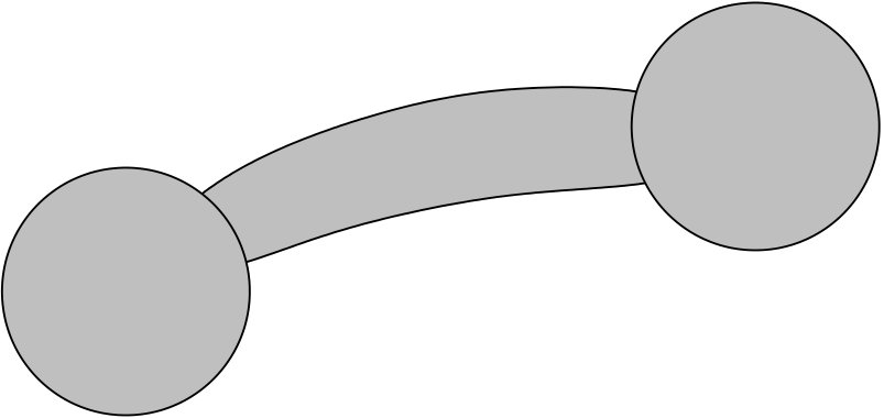 Figure 1
 Figure 2
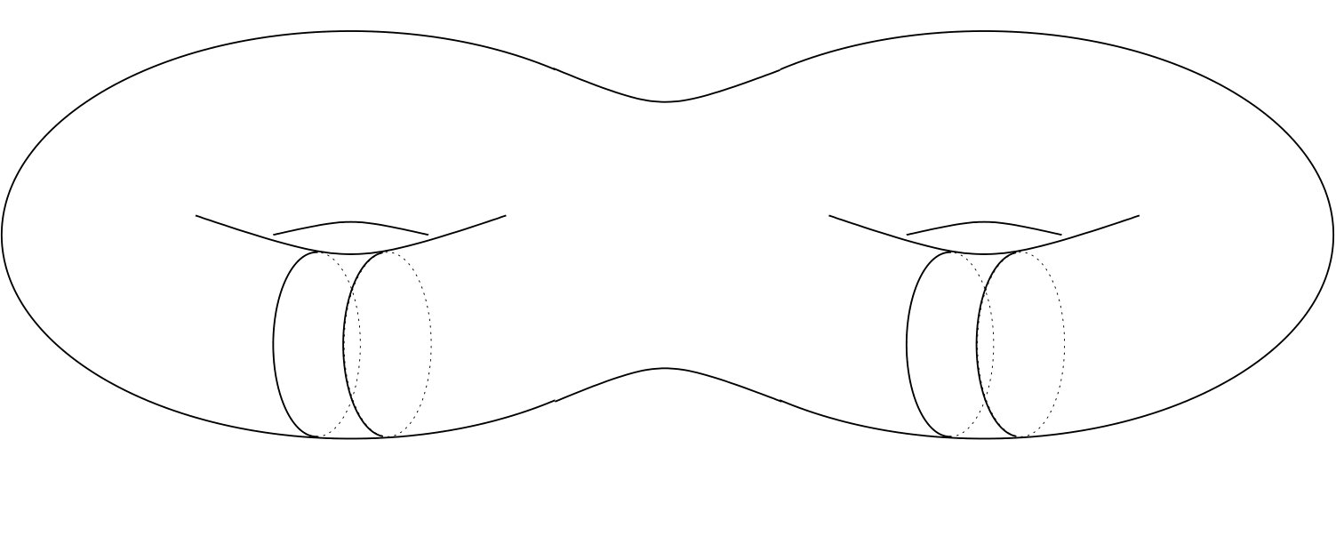 Figure 3
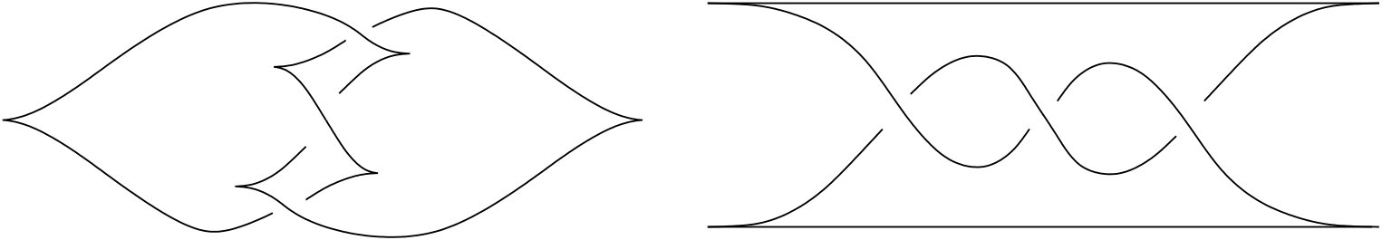 Figure 4
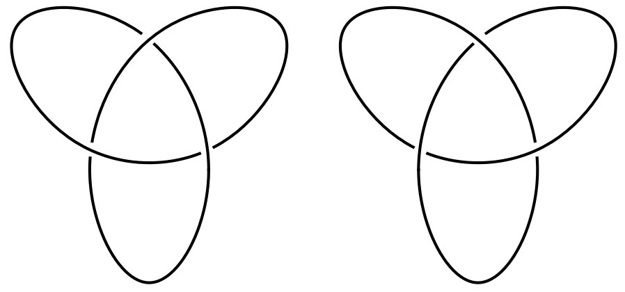 Figure 5
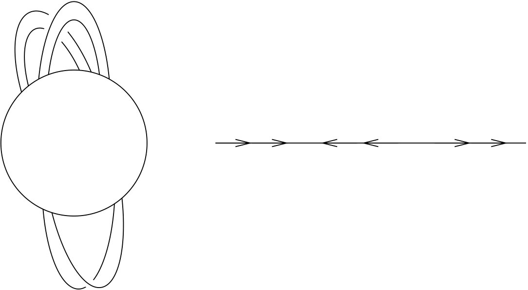 Figure 6
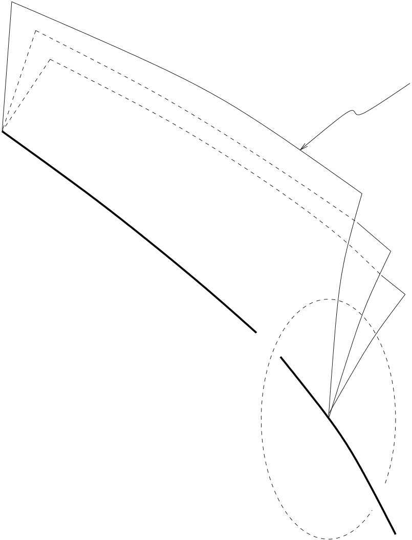 Figure 7
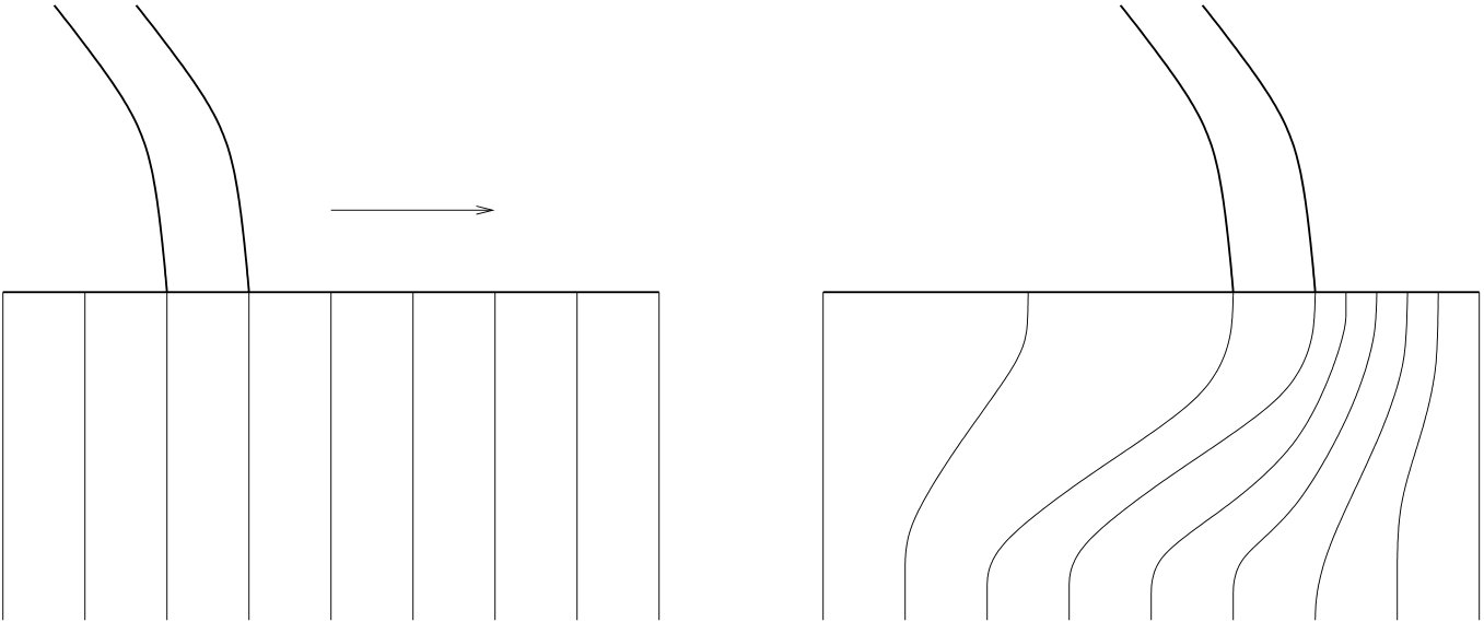 Figure 8
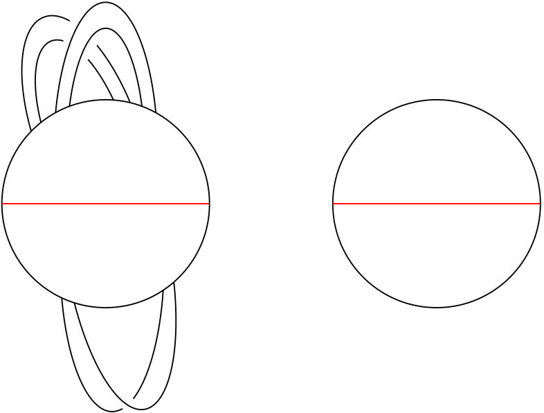 Figure 9
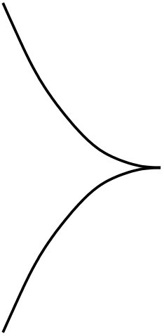 Figure 10
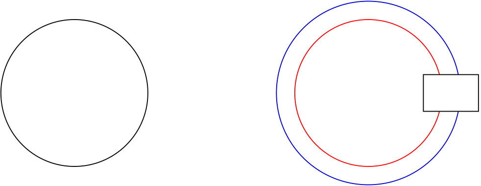 Figure 11
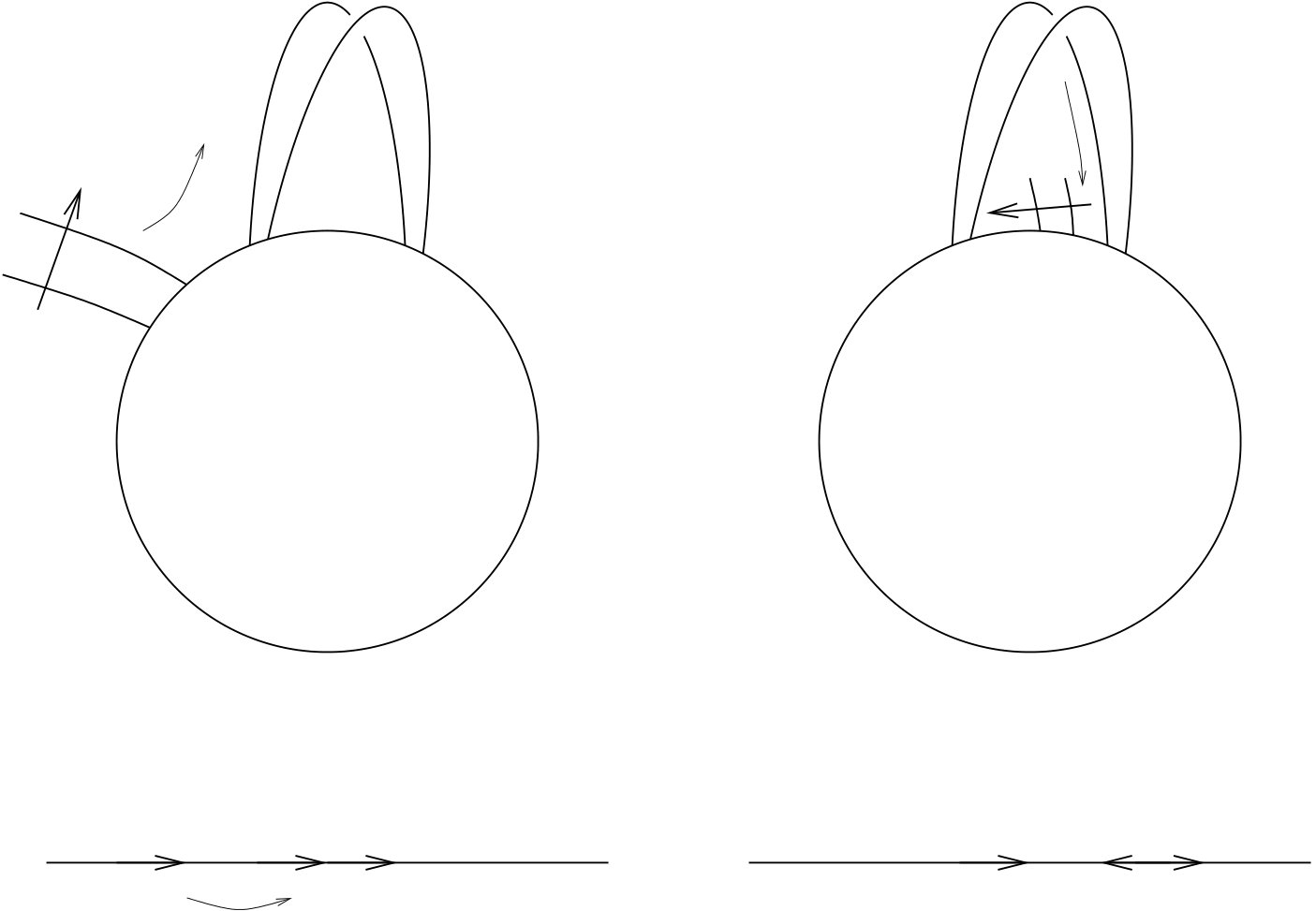 Figure 12
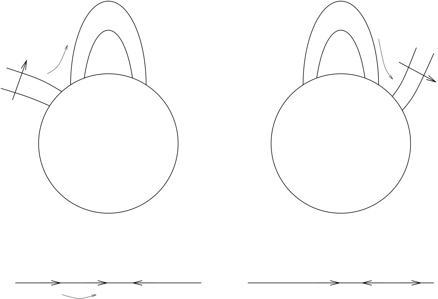 Figure 13
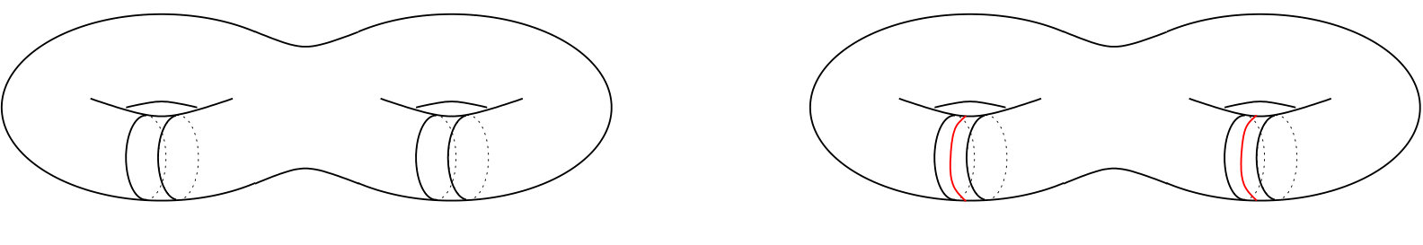 Figure 14
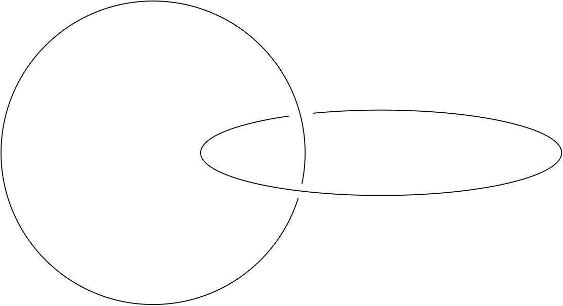 Figure 15
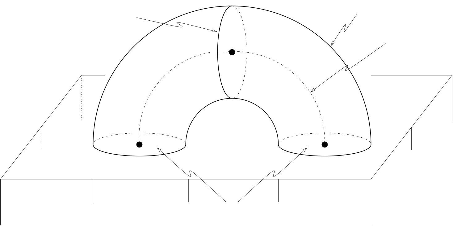 Figure 16
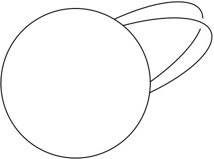 Figure 17
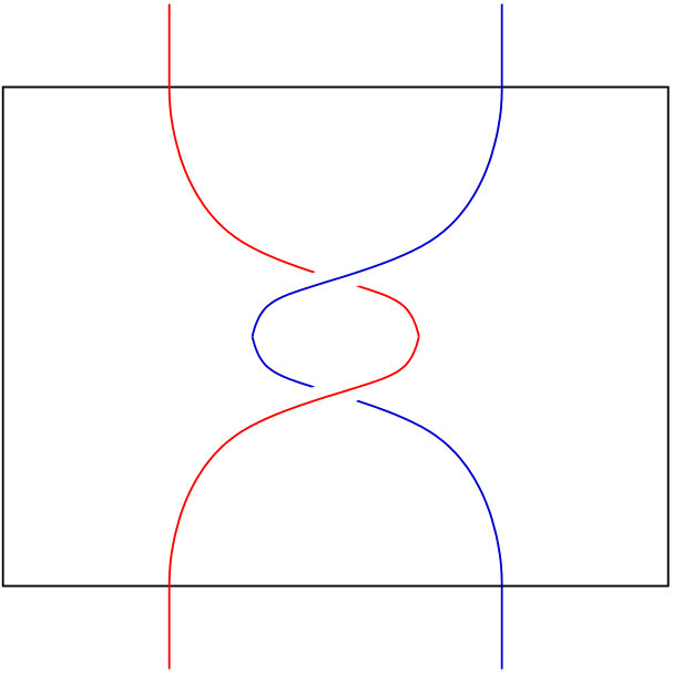 Figure 18
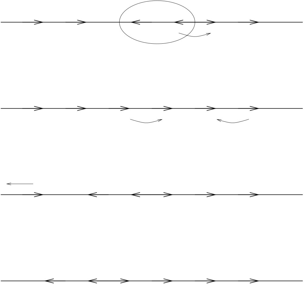 Figure 19
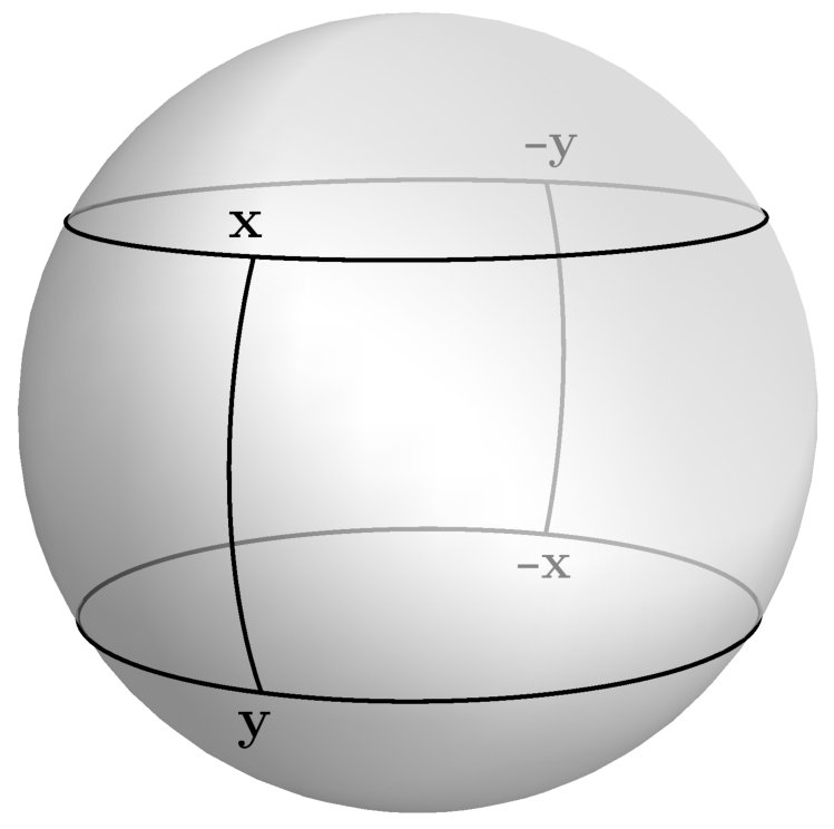 Figure 20
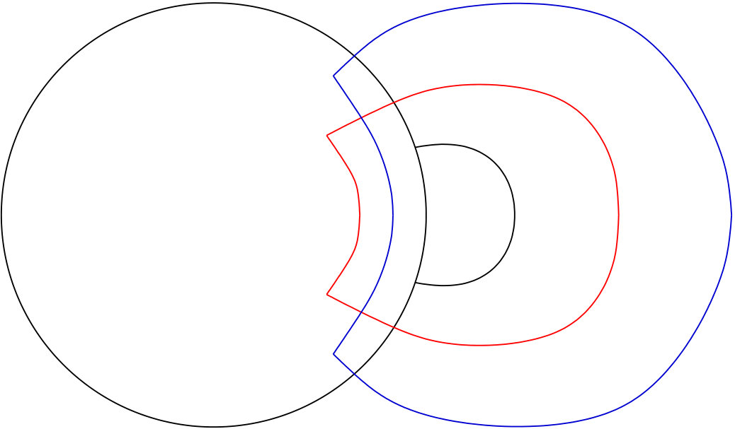 Figure 21
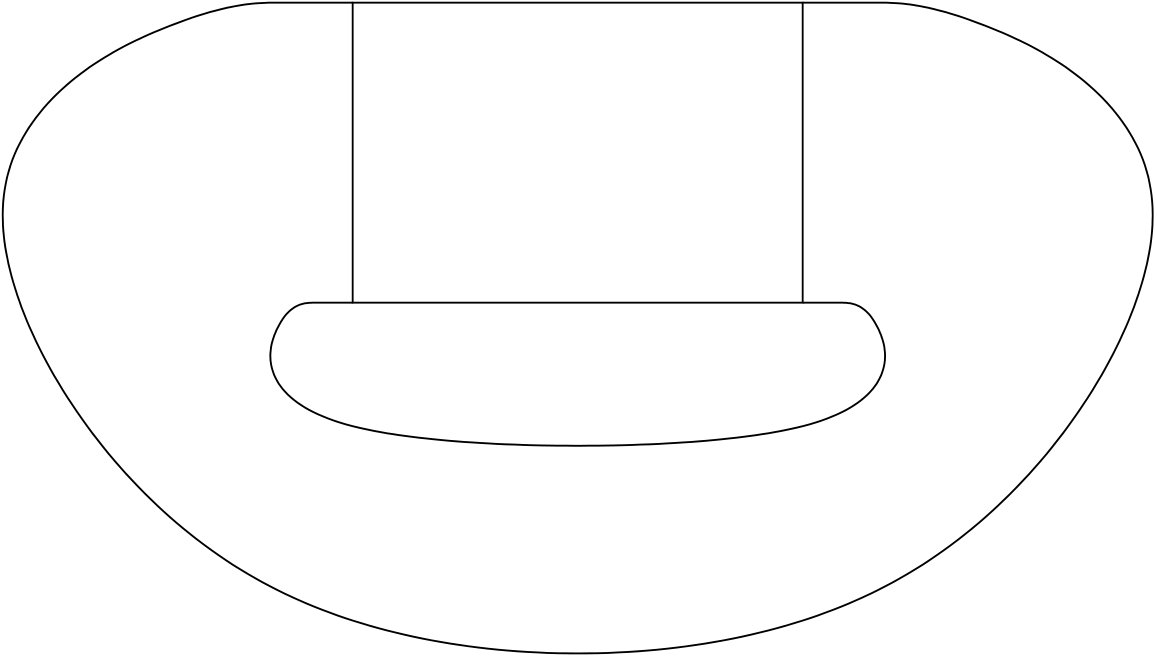 Figure 22
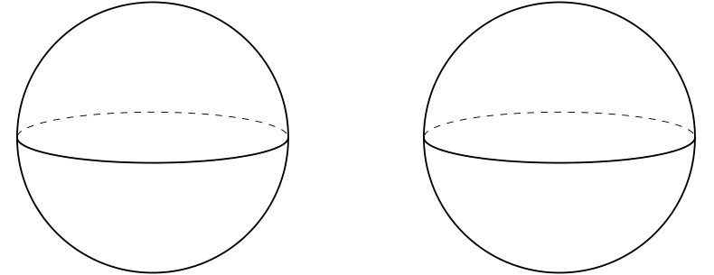 Figure 23
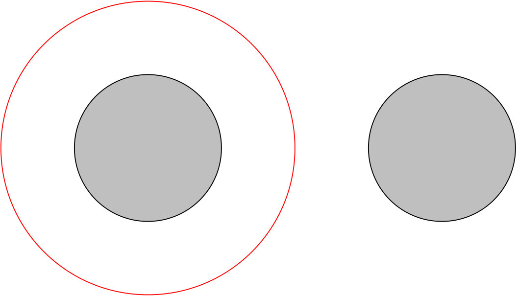 Figure 24
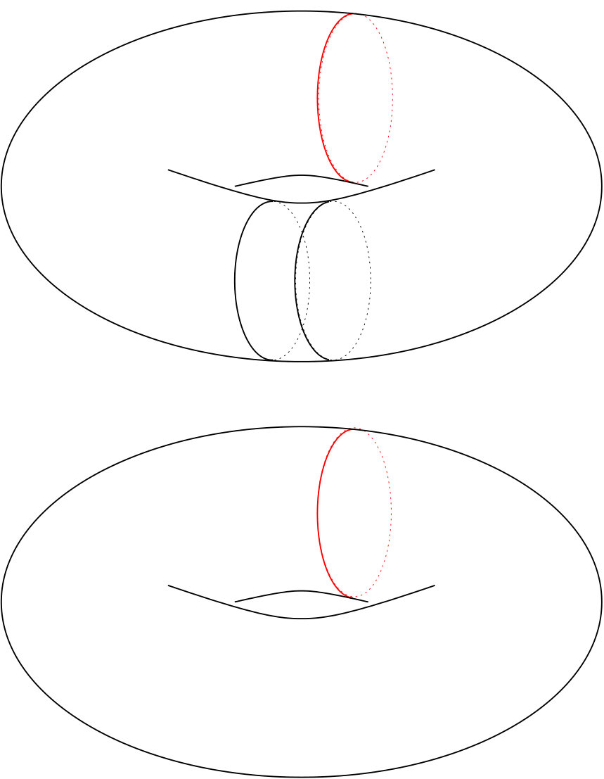 Figure 25
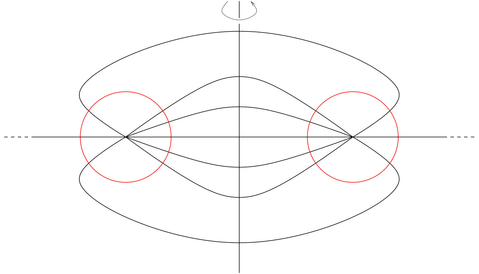 Figure 26
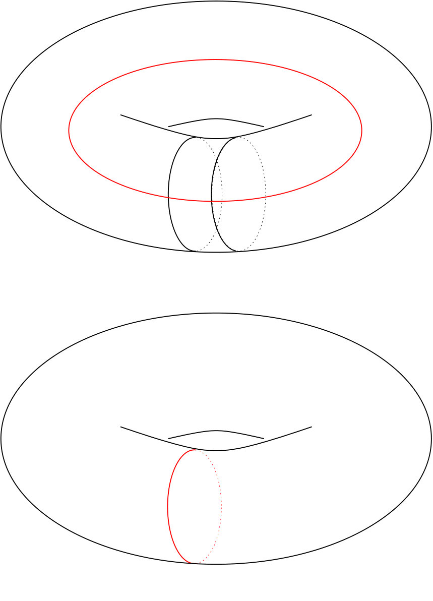 Figure 27
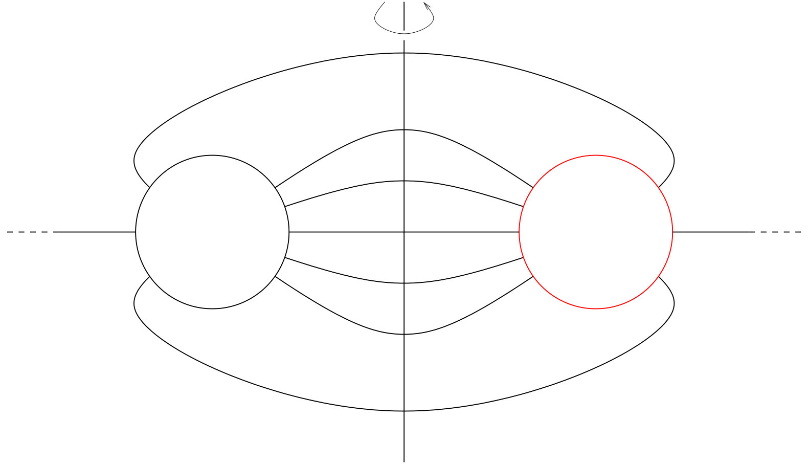 Figure 28
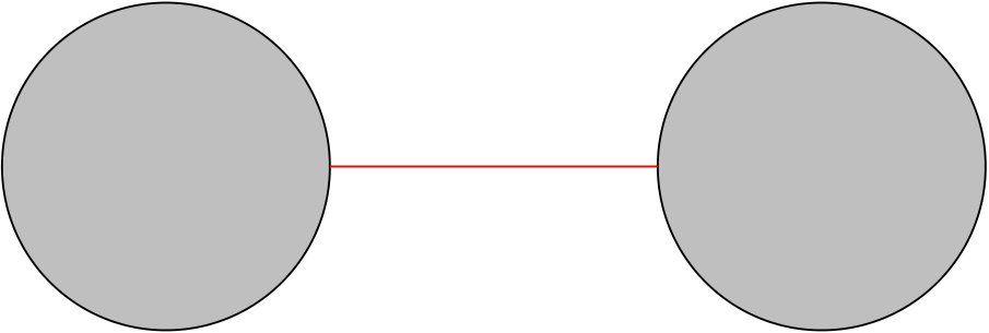 Figure 29
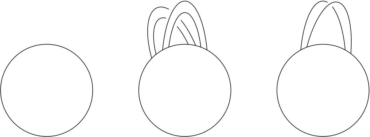 Figure 30
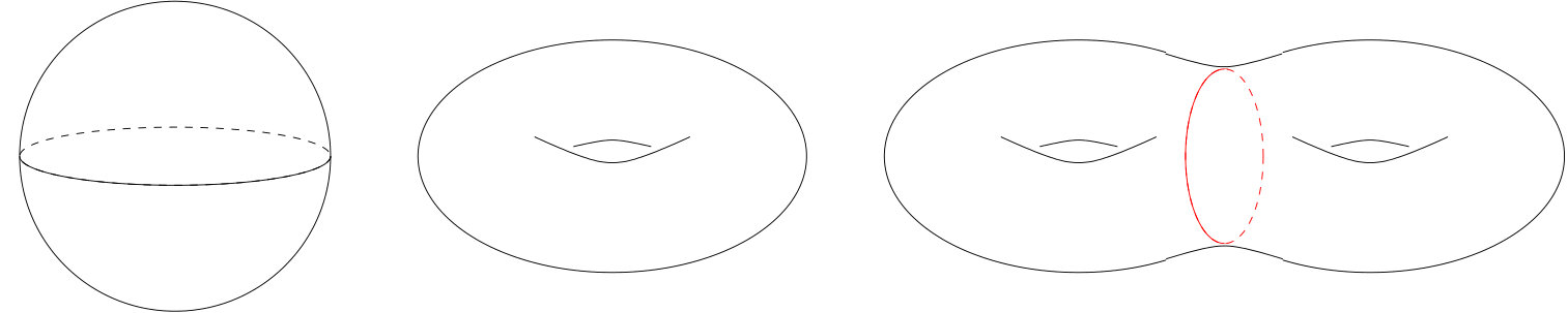 Figure 31
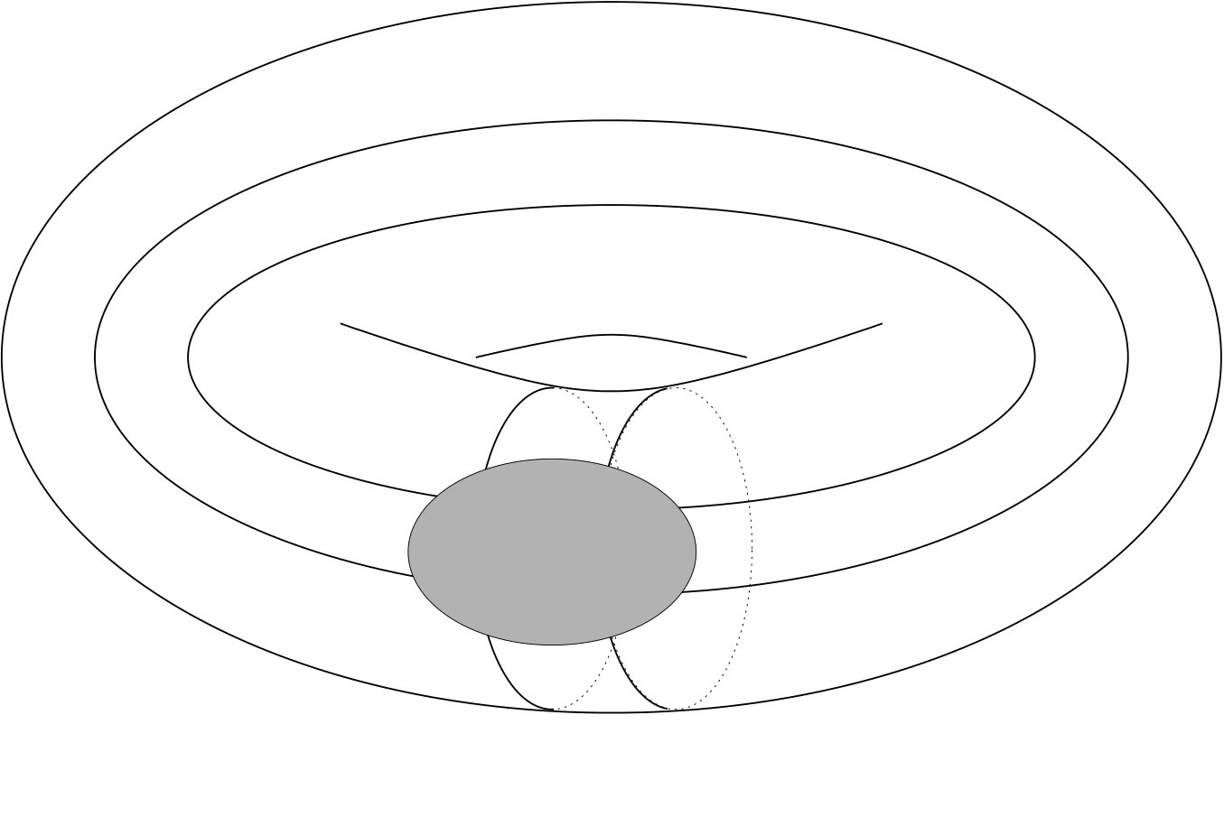 Figure 32
Peer Reviews
No public reviews on file for this paper yet. If you reviewed it on a platform where reviews are public (OpenReview, ICLR, NeurIPS, ICML), you can paste yours below so the community can read it here.
Videos
No videos yet. Explain this paper in a talk, walkthrough, or lecture? Add one.
How to depict -dimensional manifolds
Hansjörg Geiges
Mathematisches Institut, Universität zu Köln, Weyertal 86–90, 50931 Köln, Germany
Abstract.
We usually think of -dimensional manifolds as surfaces embedded in Euclidean -space. Since humans cannot visualise Euclidean spaces of higher dimensions, it appears to be impossible to give pictorial representations of higher-dimensional manifolds. However, one can in fact encode the topology of a surface in a -dimensional picture. By analogy, one can draw -dimensional pictures of -manifolds (Heegaard diagrams), and -dimensional pictures of -manifolds (Kirby diagrams). With the help of open books one can likewise represent at least some -manifolds by -dimensional diagrams, and contact geometry can be used to reduce these to drawings in the -plane.
In this paper, I shall explain how to draw such pictures and how to use them for answering topological and geometric questions. The work on -manifolds is joint with Fan Ding and Otto van Koert.
2010 Mathematics Subject Classification:
57R65, 57M25, 57R17
1. Introduction
A manifold of dimension is a topological space that locally ‘looks like’ Euclidean -space ; more precisely, any point in should have an open neighbourhood homeomorphic to an open subset of . Simple examples (for ) are provided by surfaces in , see Figure 1. Not all -dimensional manifolds, however, can be visualised in -space, even if we restrict attention to compact manifolds. Worse still, these pictures ‘use up’ all three spatial dimensions to which our brains are adapted by natural selection.
So any attempt to visualise higher-dimensional manifolds seems to be doomed. As regards -dimensional manifolds, there might be some hope to get an understanding from within, that is, if we imagine ourselves travelling inside such a space. This is not easy; even the critical Immanuel Kant seems to have taken it as a given that a space which locally looks like must needs be — at least, that’s how I interpret his dictum that the space we live in is not amenable to empirical study: “Space is not a conception which has been derived from outward experiences. […] Space then is a necessary representation a priori, which serves for the foundation of all external intuitions. […] Space is represented as an infinite given quantity.”111“Der Raum ist kein empirischer Begriff, der von äußeren Erfahrungen abgezogen worden. […] Der Raum ist eine notwendige Vorstellung, a priori, die allen äußeren Anschauungen zum Grunde liegt. […] Der Raum wird als eine unendliche gegebene Größe vorgestellt.” [13], translation from [14].
Nonetheless, one can exercise one’s imagination. A good place to start is the beautiful book by Weeks [27]. See also [22], where it is argued that Dante described an internal view of the -sphere in his Divina Commedia; cf. [5, 20]. A flight simulator for travel in various -dimensional manifolds can be found at
http://www.geometrygames.org/CurvedSpaces/index.html.en.
For more on the topology of the universe see the proceedings [26], which — rather intriguingly — contains a paper ‘Topology and the universe’ by Gott.
But how, then, is it possible to get a structural understanding of higher-dimensional manifolds if we cannot visualise them from without? The answer lies in a dimensional reduction of the representation of surfaces. I shall describe how to represent compact -dimensional manifolds by -dimensional diagrams. To ‘represent’ here means that the diagram contains complete information about the global topology of the surface. Moreover, there are rules for manipulating such diagrams that enable us to prove which diagrams represent homeomorphic surfaces.
Once this dimensional reduction has been grasped, one can proceed by analogy up to -dimensional manifolds, which should then be representable by -dimensional diagrams. Up to this point, the material presented here is classical. The -dimensional approach to the classification of surfaces, which I have not found discussed in detail elsewhere, has been tried and tested in a lecture course on the geometry and topology of surfaces.
In Section 5 I shall present a diagrammatic approach to the topology of -manifolds developed jointly with Fan Ding and Otto van Koert. The idea here is to restrict attention to a class of -manifolds that can be described as special types of so-called ‘open books’. These are decompositions of -manifolds into a collection of -dimensional ‘pages’ glued along a -dimensional ‘binding’ that constitutes the common boundary of these -manifolds (where the manifold looks like a closed half-space in ). Under suitable assumptions, it suffices to present a diagram of the -dimensional page in order to understand the topology of the -manifold. With a little help from contact geometry, as explained in the final section, we can further simplify the -dimensional diagram of the page to a -dimensional one.
This paper is an extended version of a colloquium talk I have given at a number of universities. I have tried to keep the colloquial style of the original presentation, but I have added various technical details where it seemed appropriate for a written account.
1.1. Manifolds
One usually postulates that a manifold should not only look locally like , but also that
- (M1)
is a topological Hausdorff space, i.e. any two distinct points lie in disjoint neighbourhoods, and 2. (M2)
the topology of has a countable base, i.e. there is a countable family of open subsets such that any open subset of is a union of sets from this family.
These requirements are largely a matter of technical convenience and can safely be ignored for the purposes of this paper. Condition (M1) prevents pathological examples such as a line with a double point. Take to be a copy of the real line , together with an additional point . Declare the topology on by being an open subset of , and neighbourhoods of to be sets of the form , where is a neighbourhood of the origin . This space is locally homeomorphic to , but not Hausdorff.
Condition (M2) will be redundant in this paper as we shall only be concerned with compact manifolds. In general, one imposes this condition to guarantee, for instance, metrisability of manifolds.
Examples**.**
(1) The surface of genus two in Figure 1 can be obtained from two copies of a -torus as follows: remove the interior of a small disc from each torus, then glue the resulting circle boundaries by a homeomorphism.
This operation is called a connected sum and denoted by the symbol . So is homeomorphic to . Likewise, one can define the surface of genus as the connected sum of copies of .
(2) There are surfaces that cannot so easily be visualised in -space. For instance, the real projective plane is defined as the quotient space obtained from the -sphere by identifying antipodal points. This space carries a natural topology, the so-called quotient topology, defined as follows. We have a two-to-one projection map
[TABLE]
sending each point in to its equivalence class in . A subset is called open if its inverse image is open in in the usual topology inherited from the inclusion . This defines a topology on ; it is the topology with the largest number of open sets for which the projection is continuous.
The process of gluing, as in the connected sum construction, has a similar description as a quotient. The resulting topology is the obvious one you would expect from gluing two pieces of paper along their edges.
The real projective plane is indeed a -dimensional manifold: an open neighbourhood of a point that does not contain any pair of antipodal points descends homeomorphically to a neighbourhood of .
I claim that may be thought of as the gluing of a -disc and a Möbius band along their circle boundary, see Figure 2. Think of as being made up of two polar caps, which are homeomorphic copies of , one being the antipodal image of the other. In the quotient space we can take one of these two discs to represent the equivalence classes of points coming from the polar caps. Likewise, the equivalence classes of points coming from the band around the equator are represented by points in one half of that band; when the ends of that strip are glued with the antipodal map, this creates a Möbius band. As we go once around the boundary of a polar cap, we also go once along the boundary of the Möbius band.
The real projective plane is an example of a non-orientable manifold: as one goes once along the central circle in a Möbius band, an oriented -frame returns with the opposite orientation. Moreover, the real projective plane can be realised as a surface in only at the price of allowing self-intersections. Such a realisation was discovered by T. Boy, see [12, § 47]. These two facts are correlated; an elegant argument due to Samelson [25] shows that any compact hypersurface in Euclidean space is orientable.
(3) The next surface we can construct is the connected sum . Since the removal of an open disc in leaves us with a Möbius band, this connected sum is the same as gluing two Möbius bands along the boundary. The resulting surface is known as a Klein bottle. This explains why every Klein bottle bought at kleinbottle.com comes with a product warning that, if dropped, it may shatter into two Möbius bands.
(4) In a first course on topology one learns that the connected sums , (the empty connected sum being , the neutral element for the connected sum), and , , constitute a complete list (without duplications) of the compact surfaces. Where, you may ask, is the surface or any other ‘mixed’ connected sum in that list? I shall give an answer to this question in Section 2, using the -dimensional diagrammatic language developed there.
(5) A simple example of a compact -dimensional manifold is the -sphere
[TABLE]
Stereographic projection from any point of the sphere (regarded as the north pole) onto the corresponding equatorial plane defines a homeomorphism
[TABLE]
1.2. Handle decompositions
We write for the closed -dimensional unit disc (or ball),
[TABLE]
This is a -dimensional manifold with boundary; points with have a neighbourhood in that looks like an open subset in the half-space . The boundary is denoted by ; for instance, .
Terminology**.**
In the literature, the term ‘manifold’ is often used in the wider sense so as to include manifolds with boundary. In this paper, manifolds are always understood to be without boundary, unless specified otherwise. Occasionally I shall use the standard term closed manifold for a compact manifold without boundary when I wish to emphasise those attributes.
An -dimensional -handle is a product ; the number is called the index of the handle. I suppress from the notation for the handle, as the dimension will be clear from the context. Up to homeomorphism, an -dimensional handle is of course simply a copy of the -disc ; what determines the index of a handle is how it is used to build a manifold by gluing handles.
A handle decomposition of an -dimensional manifold is a way to write it as a union of handles, where we start with a disjoint collection of -discs, which are the zero handles in the decomposition, and then successively attach handles, where a handle of index is attached to the boundary of the compound (or handlebody) of all previous handles along the part of its boundary, see Figure 3. We write for this part of the boundary and call it the lower boundary of the -handle. Similarly, we have the upper boundary . Figure 3 also shows the core disc and the belt sphere .
Thus, to attach a -handle we take an embedding
[TABLE]
i.e. a homeomorphism onto its image, and then form the quotient space , where . Notice that
[TABLE]
where the ‘corner’ is identified with its image under . In other words, the effect of a handle attachment on the boundary is to remove a copy of from and to replace it by a copy of .
Later on we shall use the following observation: If the so-called attaching sphere bounds a disc in , that disc forms together with the core disc of a -sphere in .
Here are some examples of handle attachments.
Examples**.**
(1) In the decomposition of in Figure 1 into a southern and northern hemisphere, we can regard the former as a [math]-handle and the latter as a -handle: start with a copy of and then glue another copy of along its boundary to the boundary of .
(2) A handle decomposition of the -torus into a single [math]-handle, two -handles and one -handle is shown in Figure 4.
(3) As shown before, the projective plane is obtained by gluing a -disc to a Möbius band. The latter can be written as the union of a [math]-handle and a -handle, see Figure 5. Thus, has a handle decomposition with a single [math]-, - and -handle each.
Notice that there are two ways to attach a -dimensional -handle. In the decomposition of the -torus, each -handle forms an annulus together with the [math]-handle, up to homeomorphism; we call this an untwisted -handle. In the decomposition of the projective plane, the -handle forms a Möbius band with the [math]-handle; this is a twisted -handle.
You may well ask: what if we twist a -handle twice or more? I maintain that the homeomorphism type of the resulting handlebody depends only on the number of twists being even or odd. As an example, take an untwisted annulus , which you can visualise as a a circular cylinder in . Slice it open along a segment transverse to the circular direction and then reglue it with a double twist. The obvious bijection between the annulus and the doubly twisted one is easily seen to be a homeomorphism. What has changed is the embedding of the annulus in -space, but not its intrinsic topology.
Here are some relevant facts about handle decompositions:
- (H1)
Every compact smooth manifold has a handle decomposition with finitely many handles; this is a consequence of Morse theory [19]. Here ‘smooth’ means that the coordinate change between any to local charts
[TABLE]
— the coordinate change being defined on — should be . In fact, for a handle decomposition exists even without this smoothness assumption, cf. [16, I.1]. In dimension four, the smoothness assumption is essential. 2. (H2)
If the -dimensional closed manifold is connected, one can always find a handle decomposition with precisely one handle each of index [math] and (and handles of intermediate index, unless the manifold is a sphere, cf. (H3)). Indeed, the only handle with a disconnected lower boundary is that of index . Thus, if there are several [math]-handles, the only way to arrive at a connected manifold is to connect them via -handles. But two [math]-handles connected by a -handle are homeomorphic to a single [math]-handle, see Figure 6.
For -handles one argues analogously by turning the handle decomposition ‘upside down’. Observe that we can read a handle decomposition in reverse order, where every handle of index becomes a handle of index , and the roles of lower and upper boundary are reversed.
- (H3)
The attaching of the -handle is unique up to homeomorphism (even up to diffeomorphism for ). This is a consequence of the Alexander trick: any homeomorphism of extends to a homeomorphism of by setting
[TABLE]
Thus, given a handlebody with and two gluings and , where are homeomorphisms from to , we can define a homeomorphism
[TABLE]
by setting it equal to the identity on , and equal to the extension of on . For this can be done smoothly by deep results in differential topology [15], cf. [17].
Point (H2) shows that handle decompositions of a given manifold are far from unique. Here is another cancellation phenomenon, which for simplicity I explain for surfaces: start with a -disc as a [math]-handle and attach an untwisted -handle to produce an annulus; then fill in the annulus with another -disc (acting as a -handle) to get back to a -disc. More generally, a -handle can be ‘cancelled’ by a -handle, provided it is possible to attach the latter appropriately.
From now on we shall always assume without loss of generality that the manifold in question is connected, and (in the closed case) that we have a handle decomposition with a single [math]- and -handle each.
2. Surfaces
We now apply these facts about handle decompositions to produce -dimensional representations of surfaces.
2.1. Ignore the -handle
Point (H2) allows us to assume that we have a single [math]-handle and a single -handle; point (H3) tells us that we need not care about the attaching of the -handle, so we may as well forgo drawing it. Thus, the handle decompositions in Figure 7 may be interpreted as pictures of , and , respectively.
To build connected sums of these manifolds, simply repeat the corresponding -handles along the boundary of the [math]-handle. For instance, Figure 8 shows the connected sum . I have drawn it together with the -handle so as to indicate the circle along which the connected sum splits into and .
2.2. Only draw the attaching of the -handles
As remarked upon in Section 1.2, when we have attached a -handle, in order to determine the homeomorphism type of the resulting space we need only remember where along the boundary of the [math]-handle we have attached the -handle, and whether it is a twisted or untwisted one. This allows us to encode a -handle by a pair of arrows in . Think of the arrow as coming from an orientation on the second factor in a -handle ; an untwisted handle then corresponds to the arrows pointing in opposite directions along ; a twisted arrow, in the same direction. As a further simplification, thanks to stereographic projection we can think of the circle as the union of with a point ‘at infinity’, so we may draw the arrows for the handle attachments on the real line; see Figure 9, which illustrates this for .
2.3. Handle slides
Sliding a -handle along the boundary of the handlebody to which it is attached does not change the homeomorphism type of the resulting space. This can be seen by undoing the slide in a collar neighbourhood of the boundary of the handlebody, see Figure 10.
In particular, we can slide an attaching region of a -handle across the point . In the -dimensional diagram this means that an arrow can disappear on the right, say, and reappear, pointing in the same direction, on the left.
When we slide one of the two attaching regions of a -handle along the upper boundary of a previously attached -handle , the handle receives a twist if was twisted. Notice that such a slide starts at one attaching region of and ends at the other one, at the same side of the partner arrow indicating the attachment of , see Figures 11 and 12. In either figure, one attaching region of the handle labelled slides across the handle whose attaching regions are labelled [math] and ; the slide starts at the back of the [math]-arrow and ends at the back of the -arrow.
Notice that by the same sliding argument we may assume (as we did implicitly in the preceding section) that each -handle is attached to the boundary of the [math]-handle — disjoint from the attaching regions of the other -handles — and not to parts of the upper boundary of other -handles.
The precept that every Maths talk should contain a proof applies equally to colloquia. Here is a fundamental statement on the classification of surfaces that we can now prove in diagrammatic language.
Proposition 1**.**
The surface is homeomorphic to .
Proof.
With the handle slides we discussed, the proof reduces to the three slides shown in the -dimensional diagrams of Figure 13. The diagram at the top represents ; that at the bottom, . ∎
With very similar arguments one can then show that in fact every compact surface is homeomorphic to exactly one of , , or , . I have used this approach in an undergraduate lecture course on surfaces [9], and in my view it is superior to the traditional approach to the classification of surfaces via triangulations and cut-and-paste arguments, since it extends more naturally to higher dimensions, and the steps one has to take to simplify a given word for the attaching of -handles into one of the standard words for the model surfaces are quite straightforward.
3. Dimension three: Heegaard diagrams
As we have seen, there are two ways to attach a -dimensional -handle to the boundary of a -disc. The same is true in higher dimensions. Indeed, the lower boundary of an -dimensional -handle consists of two -discs with opposite orientations. An untwisted -handle corresponds to an orientation-preserving embedding of into the boundary of the [math]-handle.
From now on I shall assume that all manifolds are orientable. This is equivalent to saying that all -handles are untwisted. The -dimensional situation is shown in Figure 14. With this assumption understood, each -handle is then simply represented by a pair of attaching discs in the boundary of the [math]-handle, i.e. the image of the lower boundary under the gluing map.
Notice that when we attach untwisted -dimensional -handles to the boundary of a -ball, the boundary of the resulting handlebody is the oriented surface of genus . Figure 15 shows an alternative view of such a handlebody (for ).
Now let be a closed -manifold. Again we appeal to (H2) and consider a handle decomposition of having precisely one [math]-handle and one -handle. Write for the handlebody made up of the [math]-handle and all (say ) -handles. This is a manifold with boundary . The complement consists of the -handles and the -handle. As observed in (H2), the -handles are glued to the -handle along their upper boundary, so we may regard this complement as a [math]-handle with -handles attached.
Since the boundary of equals that of the complement , the number of -handles must likewise be . In other words, is obtained by gluing two copies of a -handlebody of genus by a homeomorphism of their boundary , see Figure 16 (for ). Such a decomposition of a -manifold is called a Heegaard splitting.
A -handle is attached to by an embedding of the lower boundary into . Up to inessential choices, it suffices to draw the image of the central circle in , i.e. the attaching circle of the -handle. Parts of this attaching circle will lie in the upper boundary of the -handles, but we may assume that the curve traverses these upper boundaries along a straight line segment (or possibly several disjoint line segments of this form). It then suffices to draw the part of the attaching circle that lies in the boundary of the [math]-handle , outside the attaching discs of the -handles.
The final simplification comes again from regarding as the union of with a point ‘at infinity’; this allows us to draw all the information about the attaching of - and -handles in . Such a planar diagram for a -manifold is called a Heegaard diagram. Here are some simple examples.
Examples**.**
(1) The -sphere can be obtained by gluing two -balls along their boundary, that is, a -dimensional [math]-handle and a -handle. Since there are no - or -handles, this handle decomposition corresponds to the empty diagram in .
(1’) The -sphere can also be given a Heegaard splitting of any other genus. To describe the genus splitting, think of as the unit sphere in . The subset
[TABLE]
is homeomorphic to a solid torus via ; similarly, the complement is homeomorphic to via .
We regard as the union of a [math]- and a -handle; is the union of a -handle and a -handle. The gluing of and that produces the -sphere is given by the obvious identification
[TABLE]
since on .
On the boundary of a solid torus , a curve of the form is called a meridian. It is characterised (up to smooth deformations) by the fact that it is not contractible inside , but it bounds a disc in . A curve on that, when viewed as a curve in , goes once along the -factor, e.g. the curve , is called a longitude of the solid torus. In this language, the gluing of and that produces identifies a meridian of with a longitude of .
These curves are shown in Figure 17. We may think of as ; its image on is then the attaching circle of the -handle.
Alternatively, consider Figure 18. Here we think of as , and is regarded as the result of rotating the drawing plane about a vertical axis in the plane. The two discs represent the solid torus . Each line connecting the discs represents a disc; these discs make up the solid torus . Here the gluing of with is perfectly transparent.
The translation of this information into a Heegaard diagram for is shown in Figure 19. You see the attaching discs of the -handle in ; the line connecting them is the part of the attaching circle that lies outside .
(2) Another simple example of a -manifold is the product . This, too, has a Heegaard splitting of genus . Take two copies of a solid torus and identify them along the boundary with the identity map of , see Figure 20.
The identification of the two solid tori with and , respectively, can be done in such a way that the attaching circle of the -handle, i.e. the image of in , lies outside . Then the corresponding Heegaard diagram is given by Figure 21.
For more information on Heegaard splittings and diagrams see [23].
4. Dimension four: Kirby diagrams
Going up one dimension, we are hopeful to represent -dimensional manifolds by -dimensional diagrams. However, there seems to be one serious impediment. The lower boundary of a -dimensional -handle is , in other words, a thickened -sphere. Thus, in order to describe the attaching of -handles, it seems that we face the well-nigh impossible task to understand — and draw — embeddings of -spheres into the boundary of a -dimensional handlebody made up of handles of index at most .
One of the great serendipities of -manifold topology, as we shall see, is that the -handles do not, in fact, carry any topological information. This allows us to represent any closed -dimensional manifold solely by the handles of index at most .
4.1. Kirby diagrams of -handlebodies
Before I explain this phenomenon, I shall present a few examples of -dimensional -handlebodies, that is, manifolds with boundary made up of handles of index at most .
Examples**.**
(1) A -dimensional [math]-handle is simply a copy of the -disc ; its boundary is a -sphere . In order to depict the attaching of handles of higher index, we think of as , and draw the attaching regions of the handles in . These -dimensional pictures are called Kirby diagrams. Thus, the empty diagram represents the -disc.
(2) A -handle is a copy of , attached to along , i.e. two solid balls, see Figure 22. Again we assume that the two balls represent an orientation-preserving embedding of , so that the -handle is untwisted.
The schematic picture in Figure 23 shows that the manifold obtained by attaching an untwisted -handle to is homeomorphic to .
Alternatively and a little more formally, we can see this handle decomposition by splitting into two intervals , glued along two points, i.e. a [math]-dimensional sphere :
[TABLE]
(3) In order to describe the attaching of a -handle to a -dimensional handlebody , we need to visualise the image of in under the embedding used for the gluing. In the case of a -dimensional handle, it was sufficient to describe the image of , since the embedding of extends to one of in an essentially unique way.
In the -dimensional situation, however, there are homeomorphisms of that rotate the -factor as we go along the circle , and that do not extend to homeomorphisms of . Regarding as a subset of , for each integer we have the homeomorphism
[TABLE]
and we can change a given embedding by precomposing with this homeomorphism. It is not hard to see, however, that this is the only available freedom, up to inessential choices. This implies that the attaching map is determined by the image of and the parallel circle .
Figure 24 shows a right-handed twist of two curves in . A box with an integer in a diagram of knots (i.e. embedded circles) in stands for right-handed twists for , and left-handed twists for .
For instance, the Kirby diagram consisting of a single unknotted circle labelled with the integer is meant to represent the attaching of a -handle to with the images of and in as shown in Figure 25.
Now consider a schematic picture as in Figure 23, but with thought of as , and a -handle attached along the unknot . The horizontal disc and the core disc in the -handle form a -sphere . Transverse to we see copies of , so we have a well-defined projection , with the preimage of each point in equal to a -disc. This is what is called a -bundle over .
The disc in the -handle can likewise be completed to a -sphere: simply observe that the image of its boundary is another unknot in that bounds a disc. Call this -sphere .
I claim that and , after ‘wiggling’, intersect transversely in exactly points. To see this, we draw yet another schematic picture. Figure 26 shows what we should do. The image of , , bounds a disc in , which together with the disc in the -handle forms the sphere . However, instead of taking in to form the sphere, we can push it vertically into and connect it with the disc in the -handle via a vertical cylinder over . When we push deeper into than , the intersection points of and will be in one-to-one correspondence with the intersection points of and the original . With the obvious choice of , an essentially flat disc with boundary in Figure 25, there are such intersection points. One can in fact endow the -spheres with orientations and count the intersection points with sign; the correct count then will be , independent of the choice of ‘wiggling’. This number determines the -bundle over and is called its Euler number.
4.2. Kirby diagrams of closed -manifolds
When we turn our attention to closed -manifolds, we also need to comprehend the effect of attaching -handles. Regard the -handles and the single -handle as a [math]-handle with -handles attached. What does this handlebody look like?
Let us first consider the -dimensional situation. When we attach a single untwisted -dimensional -handle to a -ball, we obtain a solid torus . Attaching a further -handle amounts to starting with two solid tori and identifying a pair of -discs, one each in the boundaries of the solid tori. This construction is called a boundary connected sum, denoted by . The effect on the boundary is that of a connected sum in the old sense. Repeating this process with further -handles ( in total), we obtain the manifold with boundary .
Returning to the -dimensional situation, when we attach (untwisted) -handles to a -ball, we obtain with boundary . The felicitous fact alluded to before is the following theorem due to Laudenbach and Poénaru [18].
Theorem 2**.**
Any diffeomorphism of extends to one of .
By the argument as in Section 1 (H3), this implies that a closed -manifold is determined, up to diffeomorphism (!), by the - and -handles. Beware that the boundary of a -dimensional -handlebody will not, in general, be diffeomorphic to , so not every -handlebody corresponds to a closed -manifold. If, however, the boundary is indeed of that form, the -handlebody represents a unique closed smooth manifold.
In stark contrast with dimensions two and three, there is a subtle difference between the classification of topological and smooth -manifolds, see [11] and [16]. Some topological -manifolds do not admit any smooth structures; others, infinitely many. Strikingly, while Euclidean spaces in dimensions other than four admit a unique smooth structure, admits uncountably many distinct smooth structures, up to diffeomorphism.
It therefore deserves to be emphasised that a Kirby diagram of a closed -manifold represents a unique smooth -manifold up to diffeomorphism.
Examples**.**
(1) The -sphere is given by gluing two -balls along their boundary, that is, . So the empty Kirby diagram, read as a diagram of a closed -manifold, represents .
(2) The Kirby diagram containing a single -handle describes with boundary . Thus, in the corresponding closed -manifold we must have a single -handle, and the gluing of the two copies and of yields .
(3) The diagram in Figure 25 with represents the complex projective plane with its natural orientation coming from the complex structure. This can be seen as follows. The complement of is an open -ball: simply take to be the complex line at infinity. A neighbourhood of this complex line is a -bundle over . Consequently, is the result of attaching a -handle to this bundle space. The Euler number of the disc bundle in question being corresponds with the fact that has self-intersection equal to .
Similarly, the diagram in Figure 25 with represents , the complex projective plane with the opposite of its natural orientation.
(4) Decompose the -sphere as . Then the product -manifold splits as
[TABLE]
analogous to the handle decomposition of the -torus . The attaching circles of the -handles are and in . These are unknotted circles, since the obvious discs they bound in can be pushed to the boundary . You may convince yourself that the attaching circles are linked as shown in Figure 27; this is called the Hopf link.
The two -spheres corresponding to the -handles,
[TABLE]
and intersect in the single point . This is consistent with the argument in Figure 26, since either unknot in the Hopf link intersects the obvious disc bounded by the other one transversely in a single point. The attaching of either -handle produces a trivial -bundle or , respectively, which explains the Euler numbers [math] in Figure 27.
If one wants to study the topology of -manifolds with the help of Kirby diagrams, one needs to understand handle slides of -handles. When the attaching circle of one -handle moves across another -handle, the attaching circle twists around that of the second handle according to the Euler number of the second attaching circle, and its Euler number (or, to use the correct term in this more general context, its ‘framing’) changes by that second Euler number. You may try your hand with the following example, which is the -dimensional analogue of Proposition 1.
Proposition 3**.**
The -manifolds and are diffeomorphic.
For a comprehensive introduction to ‘Kirby calculus’, the art of manipulating Kirby diagrams, see [11].
5. Dimension five: open books
An open book decomposition of an -manifold is a way to write as a collection of -dimensional diffeomorphic submanifolds with boundary, called the pages, which are bound together along their common boundary. Take a look at Figure 28, which is essentially the Heegaard splitting of from Figure 18, except that the discs making up the solid torus in this splitting have now been extended until they touch the soul of the second solid torus . Notice that along that circle, the discs come together like the pages of a book at the binding, see Figure 29.
Here is one way to interpret this picture, giving rise to the first of two equivalent definitions of an open book decomposition.
Definition**.**
An open book decomposition of a manifold consists of a codimension submanifold , called the binding, whose neighbourhood in is required to be of the form , and a locally trivial fibration , which on B\times\bigl{(}D^{2}\setminus\{0\}\bigr{)} is given by the angular coordinate in the -factor. The closure of any fibre, , which is a codimension submanifold of with boundary , is called the page of the open book.
This definition makes perfect sense for topological manifolds, but I shall now assume that we are working in the differential category. One may then choose a vector field on transverse to the pages, equal to near the binding, and such that it projects onto the vector field on under the differential of . The time map of this vector field then defines a diffeomorphism of , equal to the identity near the boundary . This is called the monodromy of the open book.
This leads to an alternative way of viewing an open book decomposition. Start with a page and a monodromy diffeomorphism , equal to the identity near . Then form the mapping torus
[TABLE]
By the assumption on this has boundary , and we obtain a closed manifold by gluing in a copy of . The binding will then be , and the projection is given by the projection onto the second coordinate in the mapping torus, and onto the angular coordinate of the -factor in . The page in the sense of the first definition will be with a collar attached to its boundary, where corresponds to the radial coordinate in .
Example**.**
In the open book decomposition of in Figure 28 we have binding , page , and monodromy equal to .
See [28] for a beautiful survey on the history of open books and their applications to cobordism theory, foliations, differential geometry etc. All odd-dimensional closed manifolds admit an open book decomposition; manifolds of even dimension do so under some algebraic topological assumption, which in the simply connected case is the vanishing of the signature. Moreover, the pages in the decomposition of an -dimensional manifold may be assumed to have the homotopy type of a complex of dimension .
For a -dimensional manifold this means that we can always find an open book decomposition where the pages are -dimensional -handlebodies. Thus, we have a way to describe the manifold in terms of a Kirby diagram of the page, provided we can encode the monodromy diffeomorphism in this picture. This is difficult, in general, but even the identity map as monodromy gives rise to many nontrivial examples.
Examples**.**
(0) For any compact -manifold with boundary and we have
[TABLE]
(1) The empty Kirby diagram can now be read as a picture for .
(2) The diagram in Figure 22 with a single -handle and represents
[TABLE]
(3) Any -bundle over splits into two trivial bundles and , and in the bundle over the -fibres are glued over corresponding points of the equator of the base sphere by an element of the special orthogonal group varying continuously with the point on the equator. It follows that these bundles are classified by the fundamental group , so there is only the trivial bundle and a non-trivial one, denoted by . The Euler number of -bundles over that we discussed earlier can be interpreted as the corresponding element in .
It follows that the diagram in Figure 25 with represents
[TABLE]
6. Contact structures on open books
I now want to show how one can use contact geometry to achieve a further dimensional reduction: -manifolds admitting a contact structure have open book decompositions whose pages can be represented by -dimensional diagrams; if the monodromy can also be encoded in the diagram, this gives a complete description of the -manifold. At least in principle this opens the possibility that some -dimensional contact manifolds can be represented by -dimensional diagrams.
It is not my intention to give an introduction to contact geometry; for that I refer the reader to [6] or [7]. For a more detailed survey of the topics in this section see [8]. My sole aim here is to explain how contact geometry can be used to simplify at least certain Kirby diagrams to drawings in the -plane.
Definition**.**
The standard contact structure on with cartesian coordinates is the hyperplane field . In other words, is spanned by the vector fields , .
A contact manifold is an odd-dimensional manifold with a tangent hyperplane field that looks locally like .
The -sphere carries a natural contact structure, viz. the tangent field of real -planes invariant under the complex structure. The fact that this plane field is a contact structures corresponds to what complex geometers call the strict pseudoconvexity of in . On the complement of a single point, this contact structure is diffeomorphic to .
Among knots in there is the distinguished class of Legendrian knots tangent to the plane field . Consider a parametrised curve
[TABLE]
The condition for to be Legendrian is . Hence, if then . This means that the so-called front projection \gamma_{\mathrm{F}}(t)=\bigl{(}y(t),z(t)\bigr{)} does not have any vertical tangencies, but singular points instead. Away from those singularities, the missing -coordinate can be recovered from via
[TABLE]
that is, as the negative slope of the front projection in the -plane. By a -small perturbation of one can achieve that the front projection has only isolated semi-cubical cusp singularities, i.e. around a cusp at the curve looks like
[TABLE]
see Figure 30.
Notice that at a crossing of two curves in the front projection, the strand with the smaller slope will be above that with the larger one. This is illustrated in Figure 32, which shows front projections of Legendrian realisations of the left-handed and right-handed trefoil knot in Figure 31. In other words, it is superfluous to indicate the under- and overcrossings in the front projection, so we really have a strictly -dimensional picture of a knot in -space.
A Legendrian curve in a -dimensional contact manifold has a natural parallel curve, given by pushing in a direction transverse to the contact structure. For a Legendrian curve in this simply corresponds to pushing its front projection in the -direction. This parallel curve (the ‘contact framing’), with one extra left-handed twist, defines a preferred way of attaching a -handle to the -ball, and it is the one for which the complex structure on the -ball extends to a Stein structure on the -handlebody.
Recall that a Stein manifold is a complex manifold that admits a proper holomorphic embedding into some complex affine space . These admit exhausting Morse functions with strictly pseudoconvex regular level sets. Sublevel sets of this Morse function are called Stein domains, and this is what I mean by a Stein structure on a -handlebody.
A closed contact manifold is called Stein fillable if there is a Stein domain with boundary such that the tangent hyperplane field on invariant under the complex structure coincides with . The homotopical dimension of a Stein domain is always at most half of its topological dimension. If the homotopical dimension is smaller than this maximum, the Stein domain is called subcritical.
By a deep result of Giroux [10], there is an intimate relation between contact structures and open books. In dimension five this says that any contact manifold has an open book decomposition where the pages are -dimensional Stein domains, i.e. -handlebodies with the -handles attached along Legendrian knots, using the preferred framing. Thus, contact geometry leads to a further simplification: the attaching of a -handle is encoded in the Legendrian knot itself, so we no longer need to keep track of framings under handle slides.
A theory of diagrams for contact -manifolds has been developed in [2]. Here are some sample applications of this theory.
Applications**.**
(1) One can prove equivalences between contact manifolds. For instance, the manifolds and (with appropriate contact structures) are diffeomorphic. Even for the purely topological statement, the handle moves simplify by taking the contact geometric viewpoint.
(2) The diagrams can be used for a partial classification of subcritically Stein fillable contact -manifolds. For a further discussion of this issue see [3].
(3) Contact -manifolds resulting from open books with homeomorphic but non-diffeomorphic pages have been studied in [21] and [1].
(4) One can give a diagrammatic proof of the result, first shown in [4], that every simply connected -manifold admits a contact structure, provided a certain obvious topological condition (reduction of the structure group of the tangent bundle to the unitary group ) is satisfied.
(5) A purely topological application is the following. Every simply connected -dimensional spin manifold (that is, a manifold with vanishing second Stiefel–Whitney class) is a double branched cover of . This result depends in an essential way on open books with non-trivial monodromy. When a -handle is attached along an unknot, one can define a Dehn twist along the resulting -sphere in the handlebody. It turns out that all the -manifolds in question have an open book decomposition whose monodromy is a square of a diffeomorphism composed of such Dehn twists, and that the open book with the same page but monodromy is diffeomorphic to . This immediately gives the claimed branched cover description, with the binding as the branching set.
Acknowledgements**.**
I am grateful to Peter Albers and Marc Kegel for their comments on a draft version of this paper. Special thanks to Guido Sweers for creating Figures 2, 14 and 31. The research of the author is supported by the SFB/TRR 191 ‘Symplectic Structures in Geometry, Algebra and Dynamics’, funded by the Deutsche Forschungsgemeinschaft.
The reference list from the paper itself. Each links out to its DOI / PubMed record.
- 1[1] S. Akbulut and K. Yasui , Contact 5 5 5 -manifolds admitting open books with exotic pages, Math. Res. Lett. 22 (2015), 1589–1599.
- 2[2] F. Ding, H. Geiges and O. van Koert , Diagrams for contact 5 5 5 -manifolds, J. Lond. Math. Soc. (2) 86 (2012), 657–682.
- 3[3] F. Ding, H. Geiges and G. Zhang , On subcritically Stein fillable 5 5 5 -manifolds, Canad. Math. Bull. , to appear; http://dx.doi.org/10.4153/CMB-2017-011-8 .
- 4[4] H. Geiges , Contact structures on 1 1 1 -connected 5 5 5 -manifolds, Mathematika 38 (1991), 303–311.
- 5[5] H. Geiges , Mannigfaltige Geometrien, Elem. Math. 52 (1997), 93–107.
- 6[6] H. Geiges , A brief history of contact geometry and topology, Expo. Math. 19 (2001), 25–53.
- 7[7] H. Geiges , An Introduction to Contact Topology , Cambridge Stud. Adv. Math. 109 (Cambridge University Press, 2008).
- 8[8] H. Geiges , Contact structures and geometric topology, in Gobal Differential Geometry , Springer Proc. Math. 17 (Springer-Verlag, Berlin, 2012), 463–489.