Random dynamical systems generated by two Allee maps
Jozef Kov\'a\v{c}, Katar\'ina Jankov\'a

TL;DR
This paper investigates the dynamics of systems generated by two Allee maps, highlighting how their behavior varies under deterministic and stochastic conditions, especially noting significant changes with unimodal maps.
Contribution
It introduces analysis of random dynamical systems based on Allee maps, comparing behaviors with and without small random perturbations, and distinguishes effects based on map types.
Findings
Deterministic-like behavior with increasing Allee maps under randomness.
Dramatic behavioral changes in unimodal Allee maps due to stochastic perturbations.
Initial conditions have limited impact on system behavior with unimodal maps.
Abstract
In this paper, we study random dynamical systems generated by two Allee maps. Two models are considered - with and without small random perturbations. It is shown that the behavior of the systems is very similar to the behavior of the deterministic system if we use strictly increasing Allee maps. However, in the case of unimodal Allee maps, the behavior can dramatically change irrespective of the initial conditions.
Click any figure to enlarge with its caption.
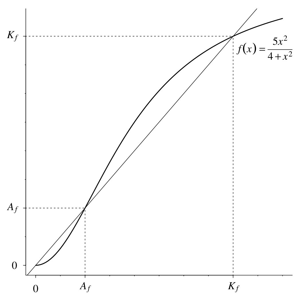 Figure 1
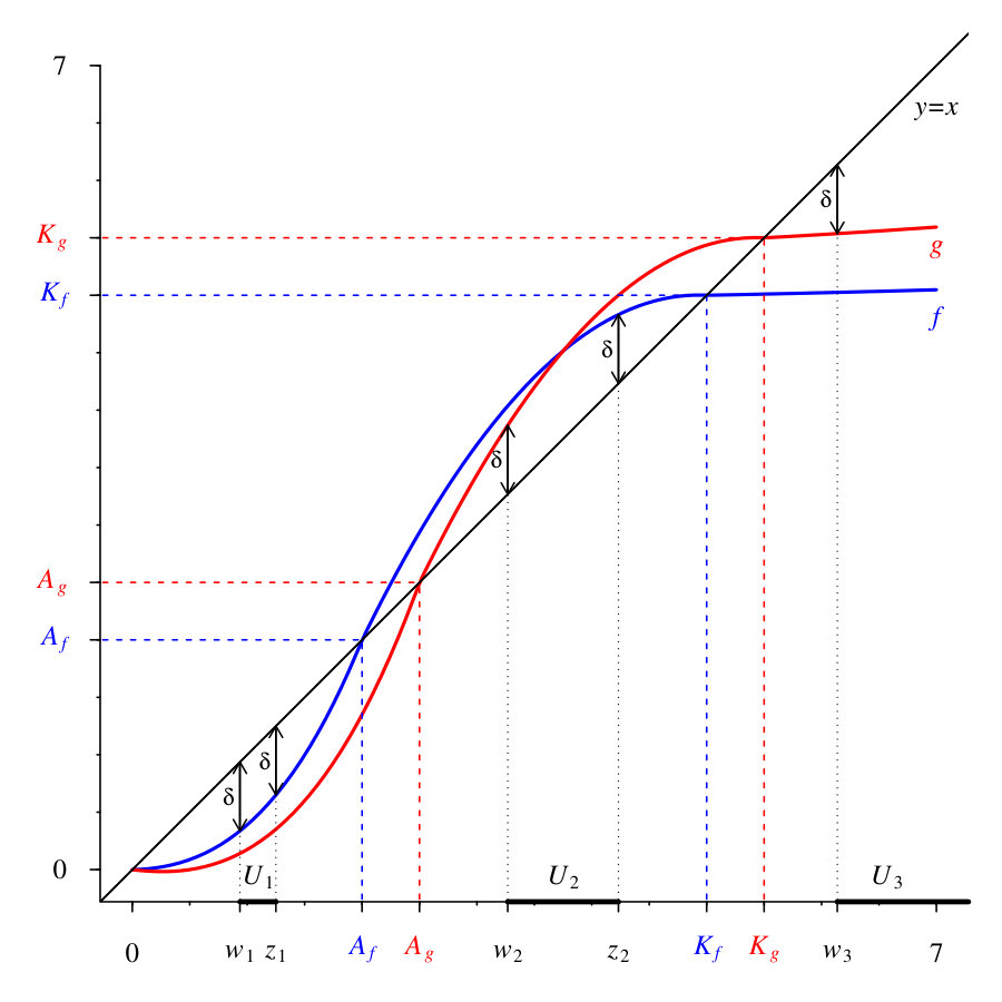 Figure 2
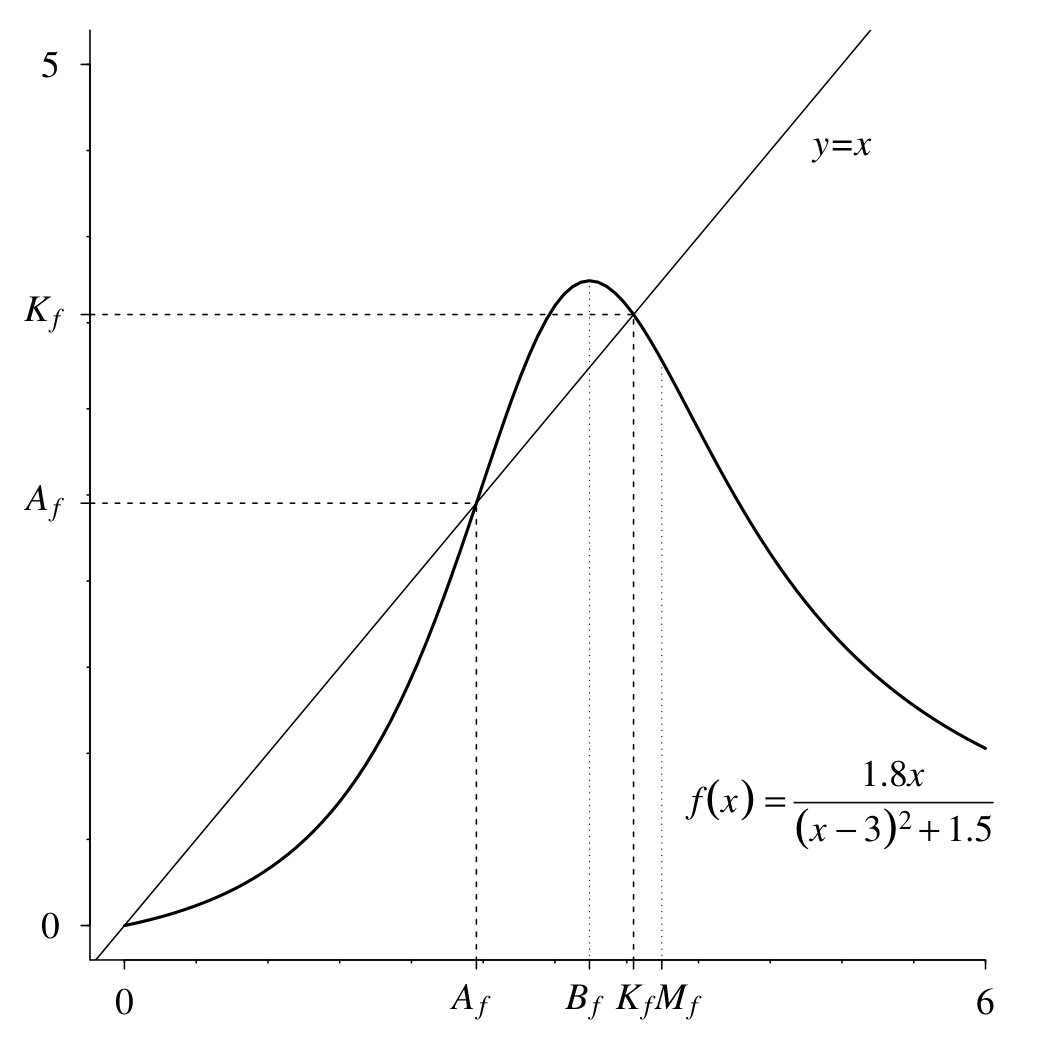 Figure 3
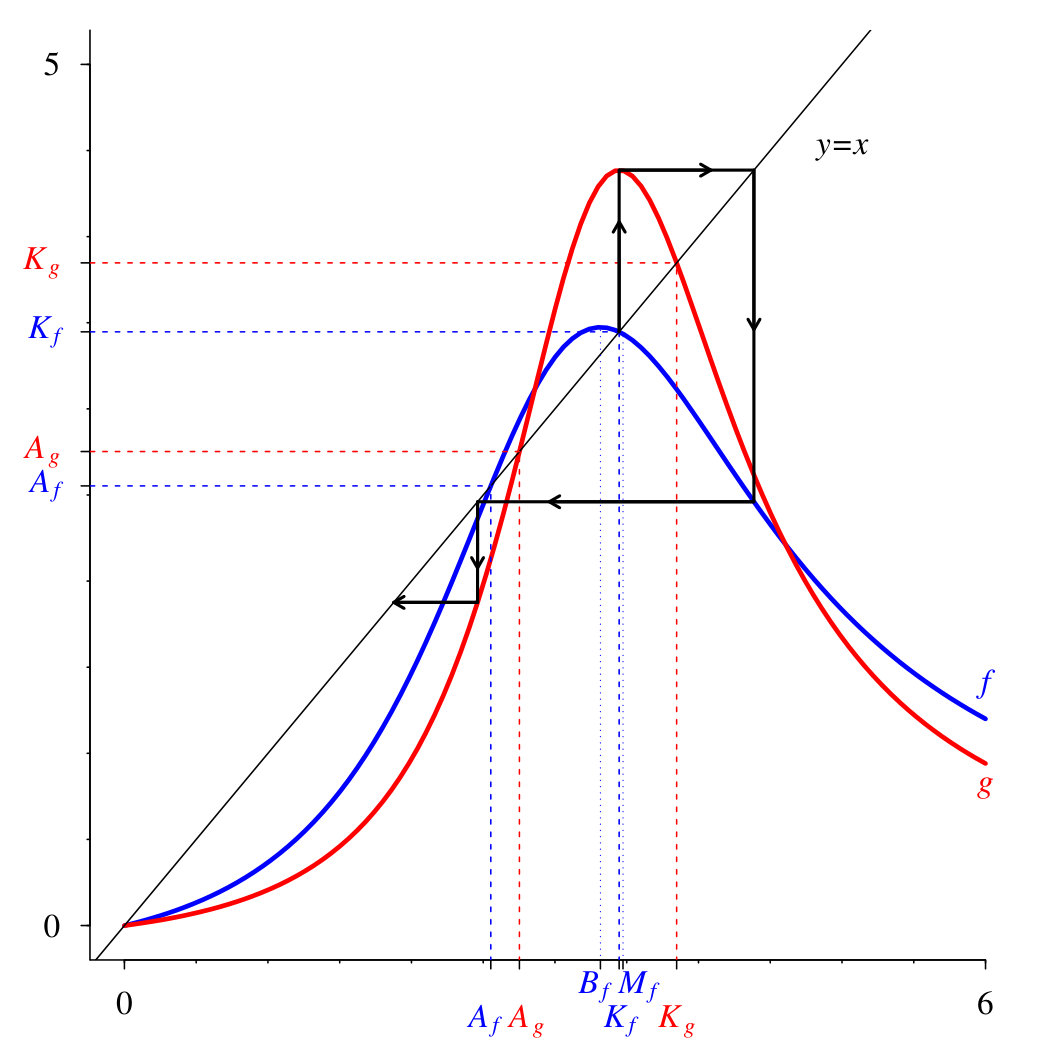 Figure 4
 Figure 5
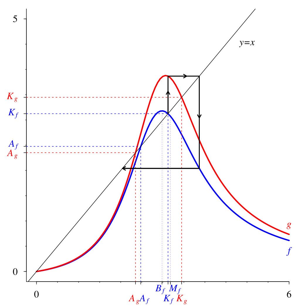 Figure 6
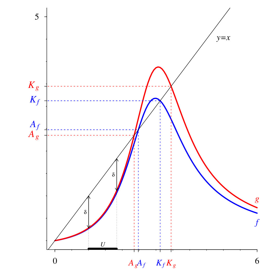 Figure 7
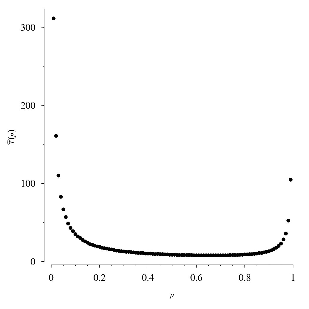 Figure 8
Peer Reviews
No public reviews on file for this paper yet. If you reviewed it on a platform where reviews are public (OpenReview, ICLR, NeurIPS, ICML), you can paste yours below so the community can read it here.
Videos
No videos yet. Explain this paper in a talk, walkthrough, or lecture? Add one.
\setkeys
Grotunits=360
Random dynamical systems generated by two Allee maps
Jozef Kováč
Department of Applied Mathematics and Statistics, Faculty of Mathematics, Physics and Informatics, Comenius University in Bratislava, Mlynská dolina
Bratislava, 84248, Slovakia
Katarína Janková
Department of Applied Mathematics and Statistics, Faculty of Mathematics, Physics and Informatics, Comenius University in Bratislava, Mlynská dolina
Bratislava, 84248, Slovakia
Abstract
In this paper, we study random dynamical systems generated by two Allee maps. Two models are considered - with and without small random perturbations. It is shown that the behavior of the systems is very similar to the behavior of the deterministic system if we use strictly increasing Allee maps. However, in the case of unimodal Allee maps, the behavior can dramatically change irrespective of the initial conditions.
keywords:
Random dynamical systems, Allee maps, Markov process
1 Introduction
The Allee effect, which was first described by W.C. Allee [1932], is a biological phenomenon characterized by a correlation between the population size and the per capita population growth rate. In the literature, the most frequently mentioned reason of this effect is the difficulty of finding mates in a smaller population (Boukal & Berec, [2002]). There are several possible scenarios for the behavior of the population size according to the strength of the Allee effect (see Boukal & Berec, [2002]).
The Allee effect was investigated from various points of view using models of dynamical and semi-dynamical systems. Interesting results were obtained for non-autonomous periodic systems. We mention several recent achievements. A special attention was given to the study of the Beverton-Holt equation. In connection with a periodic model based on this equation, two conjectures were formulated in Cushing & Henson, [2002]. These conjectures were proved in the later results of Elaydi and Sacker [2005] and also for more general systems in Kon, [2004] (see also Elaydi & Sacker, [2006]). It was shown that periodic fluctuations in the environment have, in a certain sense, a deleterious effect on the average population in the corresponding models. Periodic fluctuations in a context of economical models with an Allee effect were studied in Luís et al., [2009]. A class of unimodal Allee maps was introduced in Luís et al., [2010] where properties and stability of the three fixed points in non-autonomous periodic dynamical systems with period 2 were studied.
Some recent works take into account also randomly varying systems with the Allee effect. The stochastic stability of such systems was investigated in Haskell & Sacker, [2005] and Bezandry et al., [2008]. Environmental stochasticity in a connection with Allee effect was examined and persistence, asymptotic extinction and conditional persistence for stochastic difference equations was analyzed in Roth & Schreiber, [2014].
In this paper, only the extinction-survival scenario is studied. If the population size drops below a certain critical value, the population becomes extinct in the long run. If the size exceeds the critical value, the population is generally able to survive. Therefore the function (called an Allee map) describing population dynamics with this effect
[TABLE]
( is the population size in the -th generation) must satisfy the following conditions: {itemlist}[(3)]
has three fixed points - zero, which is a stable fixed point, an unstable threshold point and a fixed point , which can (but does not have to) be stable,
for all ,
for all .
We consider a pair of continuous Allee maps and two random dynamical systems generated by these maps. The first system is given by
[TABLE]
while the other one,
[TABLE]
contains also perturbations. In (3), are continuous i.i.d. random variables with a positive density on the interval , and is a function defined as follows:
[TABLE]
More formally (see Bhattacharya & Majumdar, [2007]), we can write , where are i.i.d. random functions such that and for some and , similarly for model (3). Given , the variable does not depend on , and thus the process is a Markov process with . The same is true for the process with .
Braverman [2011] considered a model similar to (3), i.e., with one function and scarce random perturbations. It was shown that such perturbations can, under some conditions, cause the extinction or survival of the population regardless of its initial size.
Section 2 will focus on the behavior of models (2) and (3) for strictly increasing functions and . Unimodal functions and will be analyzed in Section 3 - in both models, the population becomes extinct under some conditions, irrespective of its initial size. We can thus observe a behavior similar to the Parrondo’s paradox Harmer & Abbott, [1999].
2 Strictly increasing Allee maps
In this section, we assume that the functions and are continuous and strictly increasing. An example of such Allee map,
[TABLE]
can be found in Hoppensteadt, [1982]. It is also a special case of a new model presented in Elaydi & Sacker, [2009].
The behavior of the non-stochastic model (i.e., model (1)) is very simple. If , then and if , then . Before we formulate theorems about models (2) and (3), it is useful to mention the following lemma and its corollary.
Lemma 2.1**.**
Let be a Markov process and let for any . Assume that is such that for some and . Then .
A proof of this lemma can be found in Janková & Smítal, [1995].
Corollary 2.2**.**
Let be intervals such that the following conditions are satisfied: {arabiclist}[(2)]
* and , .*
*For any or for some .
Then .*
Theorem 2.3**.**
Let . Then {romanlist}[(iii)]
if , then ,
if , then ,
if , then , and .
Proof 2.4**.**
{romanlist}
[(iii)]
Since , for any there exists an such that . However, the function is strictly increasing, so is also strictly increasing, hence for any we have . It follows that we can apply Corollary 1 to intervals and . This can be done for an arbitrary small , hence if , then .
*If , then for all . Let us denote the set . If then and also . Hence and .
Next, , so and hence for some . Moreover, function is increasing, so it follows that for all .
Combining and Lemma 1, applied to the sets and and , we get .
If , then and we can apply Corollary 1 to the intervals and .*
*If , then and for some . Hence and .
It remains to show that . Let . Again, for some we have and since is increasing, for any . Similarly for all . Hence we can apply Lemma 1 to the sets and with .*
Theorem 2.5**.**
Let . Take a such that the sets {itemlist}[(3)]
**
**
*
are nonempty. Assume that for every there exists an such that . Then {romanlist}[(iii)]*
if , then ,
if , then ,
*if , then , and ,
where and (see Fig. 2).*
Proof 2.6**.**
{romanlist}
[(iii)]
Let . If , then we have
[TABLE]
Similar inequalities hold also for the function , hence . Similarly, if , then . Moreover, , therefore we can apply Lemma 1 to the sets and with for some .
Let and . If , then , because
[TABLE]
and
[TABLE]
similarly for the function . If , then by the assumption there exists a such that . Again, it can be shown that if , then , and so we can apply Lemma 1 (like in the case (i)) to the sets and , because . The case can be shown similarly.
*If , then the probability that for some is obviously non-zero. However, we will show in the following that also with non-zero probability for some .
Let us denote the function defined by . Since and are continuous functions, is also continuous and it follows that it attains its maximum on the interval (denote this maximum ). Next, let . Since and , it follows that , and so . Hence the probability that takes a value from is non-zero (because the density of is positive on ).
Without loss of generality, assume that , and hence (if it is not true for the function , then it is true for ). Hence with non-zero probability we have*
[TABLE]
*(the second equality is obtained by the definition of ). Similarly, we can continue with , etc. and with the same . Finally, if an is sufficiently large, with a positive probability. But if , then obviously with a non-zero probability for some .
Similarly, it can be shown that if , then with a non-zero probability for some and also for some . The case and the fact that can be shown as in Theorem 2.3.*
For or for the cases where or , very similar statements hold.
3 Unimodal Allee maps
In this section, we assume that there exists a such that the function is strictly increasing on and strictly decreasing on (denote the maximum of the function ). We also assume that the function is continuous. An example of such Allee map is the function
[TABLE]
see Asmussen, [1979].
Similarly, let be a continuous unimodal function with the maximum attained at the point . Let . For every it holds that . Thus in this section we assume that . Again, if in the deterministic model (1), then , but if , the behavior of the model can vary according to the function . However, if , a sufficient condition for the survival of the population is (in this case the population size never drops below the threshold value ).
As in Section 2, we first need the following corollary of Lemma 2.1.
Corollary 3.1**.**
Let the sets and be such that there exists with the property
[TABLE]
for some . Then
[TABLE]
(If the process returns infinitely many times to the set , then it almost surely returns infinitely many times to the set ).
Theorem 3.2**.**
Let , be differentiable and for every . Assume that there exist functions for which Then for every .
Example. Consider two functions and (see Fig 4).
Here , , and (hence ). Next, , so in this case and . Moreover, it can be shown that the function is concave on the interval , hence its first derivative is decreasing on this interval. Since and , the condition is satisfied for every . Therefore, for the process generated by these two functions, we have for every .
Proof 3.3**.**
Since is the maximum of the function , we obviously have
[TABLE]
Next, (because ) and since is continuous, there is some such that for every . Hence
[TABLE]
Denote the function defined by . This function is continuous (because and are continuous), hence there is an such that for any . Consequently
[TABLE]
Moreover, for any (since for every ), and hence there is an such that for any , and so
[TABLE]
Now we can gradually apply Corollary 3.1 to the sets {itemlist}[(4)]
* and (by (12)),*
* and (if , we can use (13) and if , then ),*
* and (by (15) and by the fact that ),*
* and (by (14)).
This means that the process returns to infinitely many times, and hence, from previous results (in Section 2), we have .*
Theorem 3.4**.**
Let , be differentiable and for every . Assume there exist functions for which . If, in addition, , then for every .
Proof 3.5**.**
Since , it follows that for some . As is continuous, we have
[TABLE]
*for some . Since , two cases are possible: either or .
If , then for some and from the continuity of , we have for any , where .*
Consequently
[TABLE]
Again, we can apply Corollary 3.1 to the sets {itemlist}[(5)]
* and (by (12)),*
* and (by (17) if and by the fact, that if ),*
* and (as in the preceding theorem),*
* and (by (16), because ),*
* and (since , and so for some for an arbitrary ).
It follows that the process returns to the set infinitely many times, hence .
If , then for some and also (since is the maximum of the function ). Therefore*
[TABLE]
where . The rest of the proof is similar to the proof of the first case.
Example. Let and (see Fig. 6).
Here and (hence ). Further, and . Moreover, the function is again concave on and , hence for every . Thus, from Theorem 3.4 it follows that .
Since for every and for an arbitrary , the population persists in the deterministic model (model (1)) generated by the function ; similarly the population persists in the model generated by . However, if we combine these models, the population becomes almost surely extinct. This resembles results known as the Parrondo’s paradox (see e.g. Harmer & Abbott, [1999]).
A very similar theorem holds for the process .
Theorem 3.6**.**
Let be a differentiable function and for an arbitrary . Assume there exist functions for which . If, in addition, the set
**
is nonempty (see Fig. 7), then for every .
The proof is almost the same as the proof of Theorem 3.2 and Theorem 3.4 - inequality (12) can be modified to
[TABLE]
similarly for inequality (13). Inequality (14) can be shown as follows:
Suppose that for some (the proof is the same for functions). Since is continuous, we have for an arbitrary for some . Next, from the continuity of , there exists an such that for every . Now let . Then and since is an open set, there exists a such that . It follows that
[TABLE]
Next, if , then , and so there exists a such that . Hence we obtain
[TABLE]
Inequalities (15), (16), (17) and (18) can be shown similarly - from the continuity of the functions and and by the fact that the density of is positive on .
Remark. The condition in Theorem 3.4 is not necessary in this case - Corollary 3.1 can be applied directly to the sets and .
4 Concluding remarks
{arabiclist}
[(5)]
In Section 2, we showed that models (2) and (3) lead to similar results as the deterministic model, if we work with two strictly increasing Allee maps (recall that we distinguish only between extinction and survival here). If the initial population size is greater than some threshold, the population persists; if it is smaller than another threshold, the population becomes extinct. The only difference from the non-stochastic case is the region between these two thresholds - if the initial population size is in this region, both scenarios (extinction or survival) are possible.
In Theorems 2.3 and 2.5 only the inequality was considered. If the order of these values is different, proofs and results are very similar. The only difference is in the case (or ). For these two orderings of the values, it can be easily shown that the population becomes almost surely extinct.
If does not satisfy the conditions of Theorem 2.5 or Theorem 3.6 (i.e. can take relatively high values), then it is not possible to predict the long-term behavior of the system. Its values can increase even from zero to high numbers and vice versa.
In Section 3, we showed that under some conditions the population becomes almost surely extinct. This is caused by the fact that the population size almost surely drops below the critical value , which leads to the extinction. Therefore, it would be interesting to calculate the expected value of the time after which the system drops below this critical value. Generally, this can be a very difficult problem, because this time depends on the given functions and and also on the probability with which we choose functions and . However, if we fix the functions and the probability, the expected time can be estimated by simulations. We examined the expected time in the case where the functions were the same as in the second example for different probabilities and for . As previously mentioned (in the second example), if we consider only one function ( or ), the population size never drops below the critical value, hence for and . For the estimates are shown in Fig. 8. A question is whether it is possible to calculate these values exactly and in more general situations.
In Section 3, we considered only specific conditions for unimodal Allee maps, which have interesting consequences. It would be interesting to study other situations.
\nonumsection
Acknowledgments Supported by the VEGA Grant No. 2/0047/15 from the Slovak Scientific Grant Agency (Kováč, Janková) and the UK/344/2016 grant from Comenius University in Bratislava (Kováč).
The reference list from the paper itself. Each links out to its DOI / PubMed record.
- 1Allee, [1932] Allee, W. C. [1932] “Studies in animal aggregations: mass protection against colloidal silver among goldfishes,” J. Exp. Zool. 61 , pp. 185–207.
- 2Asmussen, [1979] Asmussen, M. A. [1979] “Density-dependent selection II. The Allee effect,” Am. Nat. 114 , pp. 796–809.
- 3Bezandry et al. , [2008] Bezandry, P. H., Diagana, T. & Elaydi, S. [2008] “On the stochastic Beverton- Holt equation with survival rates, ” J. Difference Equ. Appl. 14 , pp. 175–190.
- 4Bhattacharya & Majumdar, [2007] Bhattacharya, R. & Majumdar, M. [2007] Random Dynamical Systems: Theory and Application (Cambridge University Press, Cambridge).
- 5Boukal & Berec, [2002] Boukal, D. S. & Berec, L. [2002] “Single-species models of the Allee effect: extinction boundaries, sex ratios and mate encounters,” J. Theor. Biol. 218 , pp. 375–394.
- 6Braverman, [2011] Braverman, E. [2011] “Random perturbations of difference equations with Allee effect: switch of stability properties,” Proceedings of the Workshop Future Directions in Difference Equations, Colecc. Congr. (Univ. Vigo, Serv. Publ., Vigo, 2011) 69 , pp. 51–60.
- 7Cushing & Henson, [2002] Cushing, J. M. & Henson, S. M. [2002] “A periodically forced Beverton-Holt equation,” J. Difference Equ. Appl. 8 , pp. 1119–1120.
- 8Elaydi & Sacker, [2005] Elaydi, S. N. & Sacker, R. J. [2005] “Global stability of periodic orbits of non-autonomous difference equations and population biology,” J. Differential Equations 208 , pp. 258–273.