Aerosols optical properties in Titan's Detached Haze Layer before the equinox
Beno\^it Seignovert, Pascal Rannou, Panayotis Lavvas, Thibaud Cours,, Robert A. West

TL;DR
This study analyzes Titan's detached haze layer using Cassini UV observations, revealing stable aerosol properties over time in the southern hemisphere and size variations in the northern hemisphere, with implications for understanding Titan's atmospheric aerosols.
Contribution
It introduces a method to extract aerosol optical properties from high-resolution UV images and demonstrates their stability and variability across Titan's hemispheres over several years.
Findings
Aerosols consist of at least ten 60 nm monomers.
Aerosol properties are stable in the southern hemisphere.
Northern hemisphere aerosols tend to decrease in size and increase in opacity.
Abstract
UV observations with Cassini ISS Narrow Angle Camera of Titan's detached haze is an excellent tool to probe its aerosols content without being affected by the gas or the multiple scattering. Unfortunately, its low extent in altitude requires a high resolution calibration and limits the number of images available in the Cassini dataset. However, we show that it is possible to extract on each profile the local maximum of intensity of this layer and confirm its stability at km during the 2005-2007 period for all latitudes lower than 45N. Using the fractal aggregate scattering model of Tomasko et al. (2008) and a single scattering radiative transfer model, it is possible to derive the optical properties required to explain the observations made at different phase angles. Our results indicates that the aerosols have at least ten monomers of 60 nm radius, while the typical…
Click any figure to enlarge with its caption.
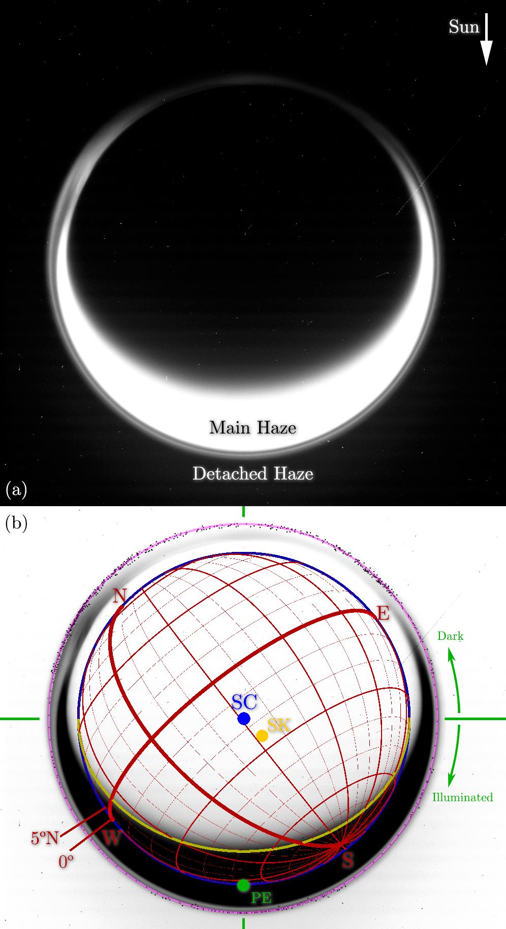 Figure 1
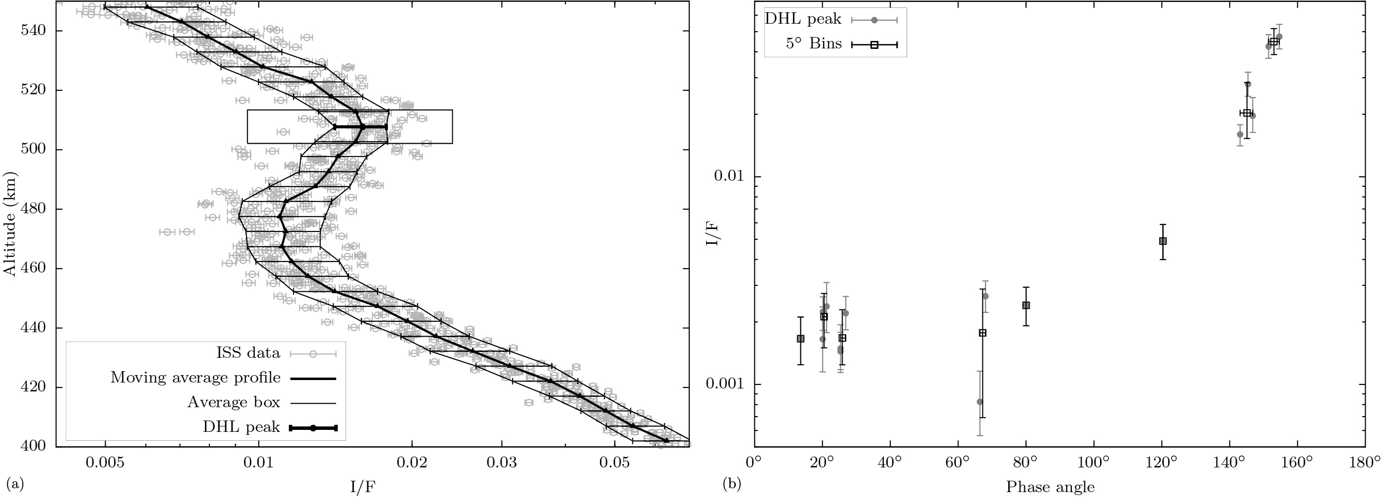 Figure 2
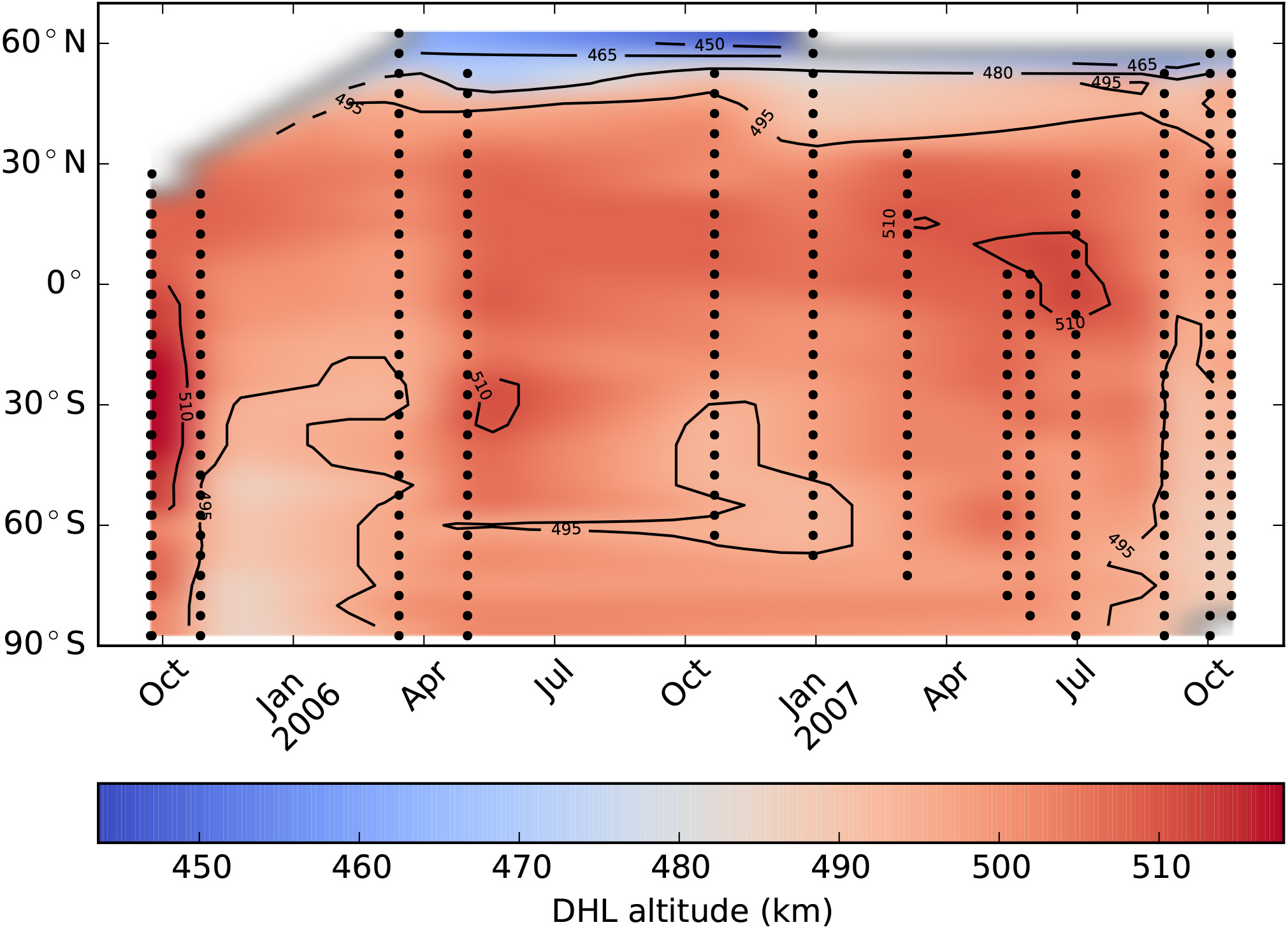 Figure 3
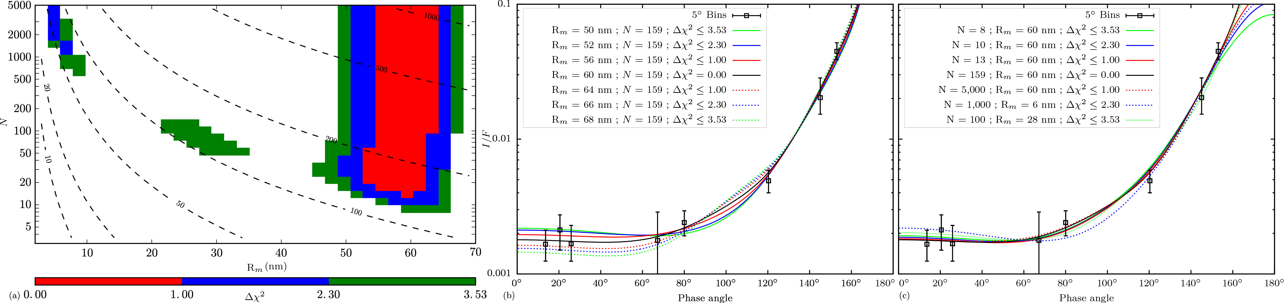 Figure 4
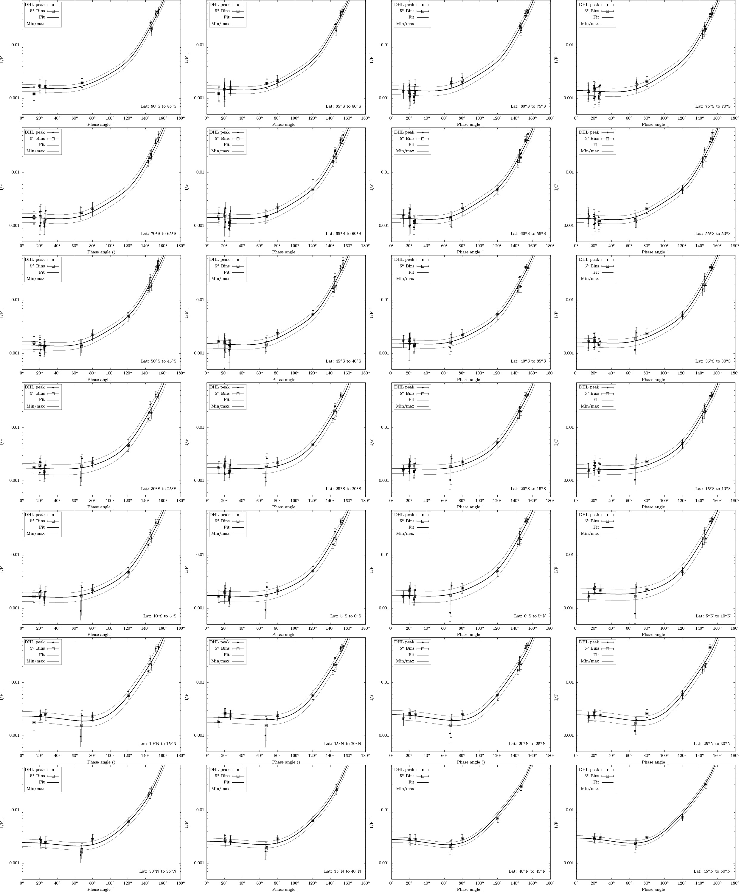 Figure 5
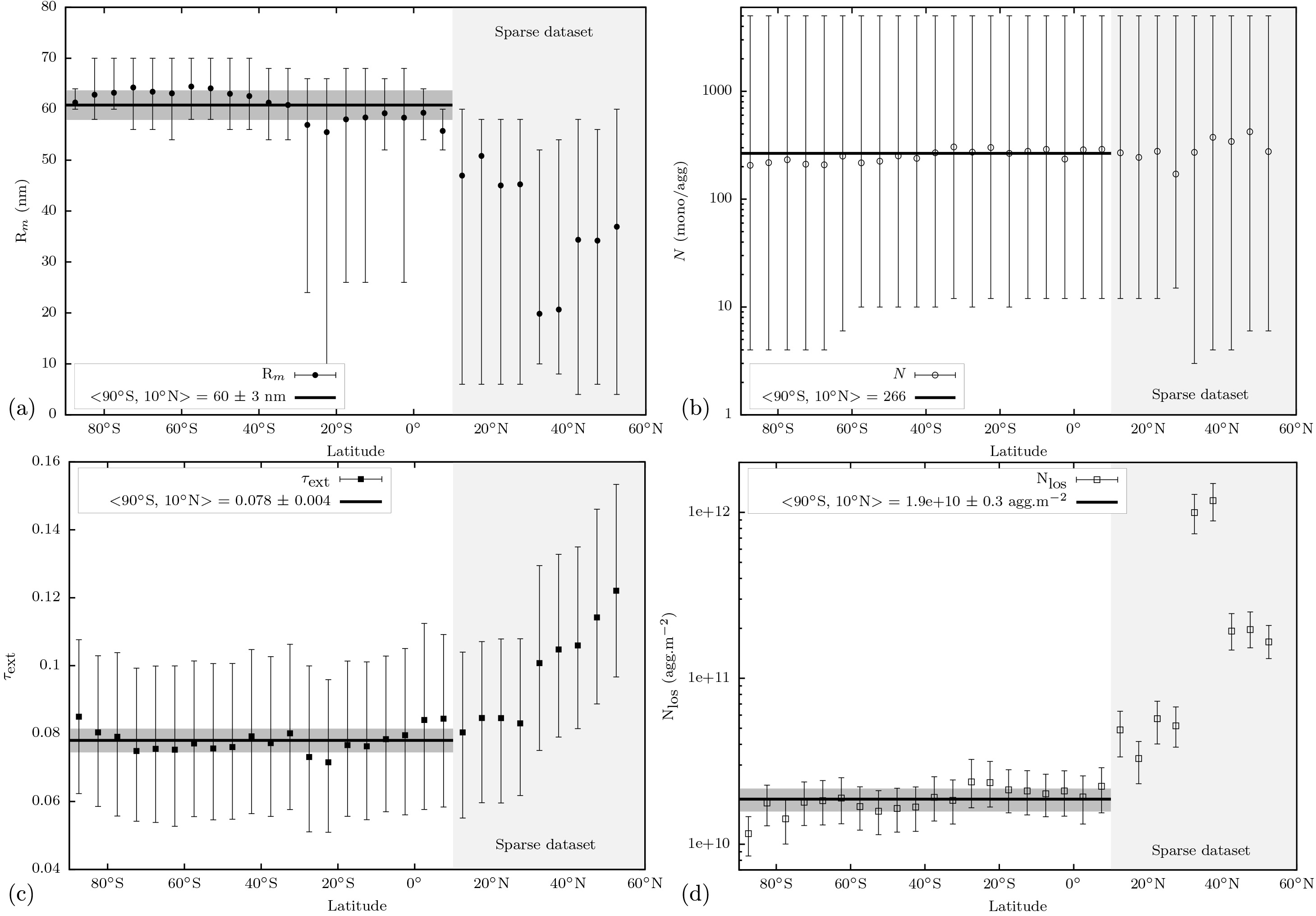 Figure 6
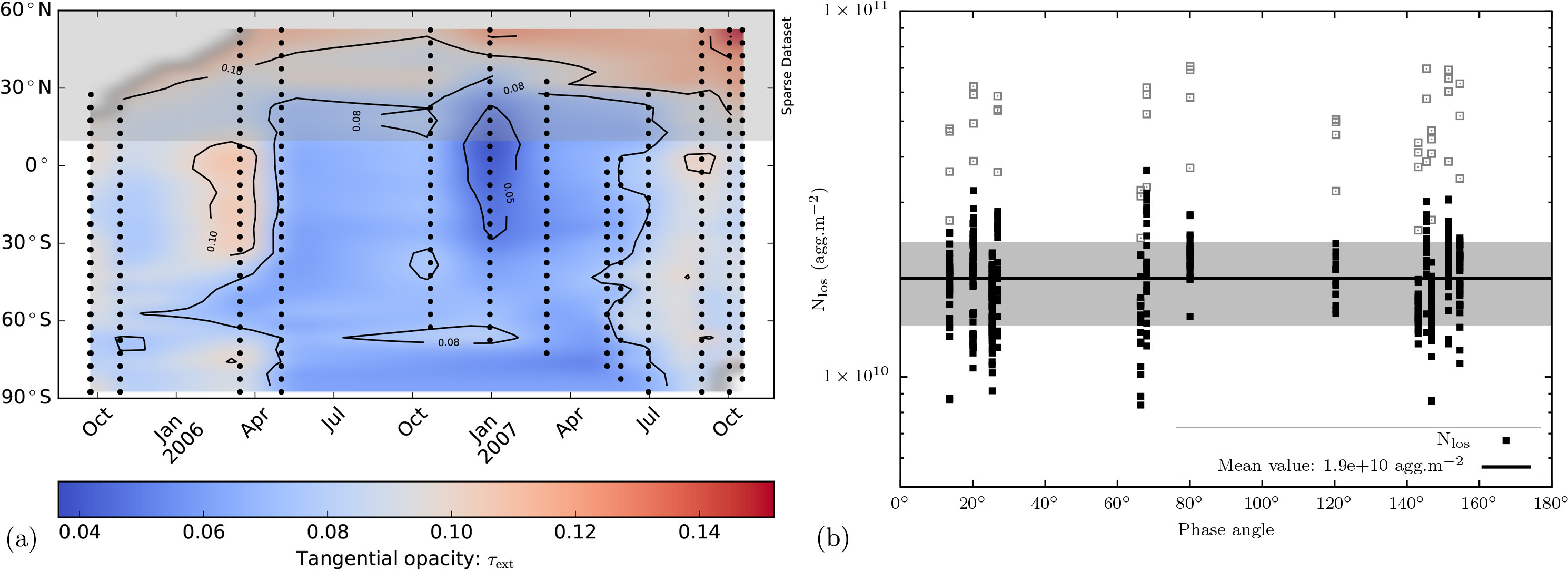 Figure 7
| ISS ID | Date | Phase | Coverage | Lat. Photo. | Pixel scale (km) |
|---|---|---|---|---|---|
| N1506288442_1 | 2005/09/24 | 145∘ | 90∘S-25∘N | 37∘S | 5.5 |
| N1506300441_1 | 2005/09/25 | 151∘ | 90∘S-30∘N | 46∘S | 5.5 |
| N1509304398_1 | 2005/10/29 | 155∘ | 90∘S-25∘N | 51∘S | 6.1 |
| N1521213736_1 | 2006/03/16 | 68∘ | 90∘S-65∘N | 19∘S | 7.3 |
| N1525327324_1 | 2006/05/03 | 147∘ | 90∘S-55∘N | 33∘S | 7.2 |
| N1540314950_1 | 2006/10/23 | 120∘ | 65∘S-55∘N | 2∘S | 5.7 |
| N1546223487_1 | 2006/12/31 | 66∘ | 70∘S-65∘N | 6∘S | 7.4 |
| N1551888681_1 | 2007/03/06 | 143∘ | 75∘S-35∘N | 49∘S | 7.9 |
| N1557908615_1 | 2007/05/15 | 25∘ | 80∘S-10∘N | 76∘S | 7.8 |
| N1557919415_1 | 2007/05/15 | 25∘ | 80∘S-10∘N | 75∘S | 8.2 |
| N1559282756_1 | 2007/05/31 | 20∘ | 85∘S-10∘N | 80∘S | 7.7 |
| N1562037403_1 | 2007/07/02 | 14∘ | 90∘S-30∘N | 58∘S | 7.8 |
| N1567440117_1 | 2007/09/02 | 20∘ | 90∘S-55∘N | 22∘S | 7.9 |
| N1570185840_1 | 2007/10/04 | 27∘ | 90∘S-60∘N | 28∘S | 7.3 |
| N1571476343_1 | 2007/10/19 | 80∘ | 85∘S-60∘N | 11∘S | 8.2 |
| Parameter | Symbol | Value | Std | Unit |
|---|---|---|---|---|
| Monomer radius | Rm | 60 | 3 | nm |
| Number of monomer per aggregate | 266 | - | - | |
| Aggregate bulk radius | Rv | 0.4 | - | m |
| Tangential opacity | 0.078 | 0.004 | - | |
| Tangential column number density | Nlos | 1.9 | 0.3 | m-2 |
| Parameter | Symbol | Value | Unit |
| Scattering cross-section | 2.9e-12 | m2 | |
| Extinction cross-section | 4.2e-12 | m2 | |
| Absorption cross-section | 1.3e-12 | m2 | |
| Single-scattering albedo | 0.69 | - | |
| Phase function: = 0∘ | - | 185.8 | - |
| = 1∘ | - | 178.1 | - |
| = 2∘ | - | 157.2 | - |
| = 4∘ | - | 98.9 | - |
| = 6∘ | - | 52.6 | - |
| = 8∘ | - | 28.4 | - |
| = 10∘ | - | 17.4 | - |
| = 15∘ | - | 8.0 | - |
| = 20∘ | - | 4.7 | - |
| = 30∘ | - | 2.2 | - |
| = 40∘ | - | 1.1 | - |
| = 50∘ | - | 0.58 | - |
| = 60∘ | - | 0.36 | - |
| = 80∘ | - | 0.21 | - |
| = 100∘ | - | 0.144 | - |
| = 120∘ | - | 0.117 | - |
| = 140∘ | - | 0.112 | - |
| = 160∘ | - | 0.115 | - |
| = 180∘ | - | 0.117 | - |
Peer Reviews
No public reviews on file for this paper yet. If you reviewed it on a platform where reviews are public (OpenReview, ICLR, NeurIPS, ICML), you can paste yours below so the community can read it here.
Videos
No videos yet. Explain this paper in a talk, walkthrough, or lecture? Add one.
Aerosols optical properties in Titan’s Detached Haze Layer before the equinox
Benoît Seignovert
Pascal Rannou
Panayotis Lavvas
Thibaud Cours
Robert A. West111Visiting at GSMA/URCA
GSMA, Université de Reims Champagne-Ardenne, UMR 7331-GSMA, 51687 Reims, France
Jet Propulsion Laboratory, California Institute of Technology, Pasadena, CA 91109, USA
Abstract
UV observations with Cassini ISS Narrow Angle Camera of Titan’s detached haze is an excellent tool to probe its aerosols content without being affected by the gas or the multiple scattering. Unfortunately, its low extent in altitude requires a high resolution calibration and limits the number of images available in the Cassini dataset. However, we show that it is possible to extract on each profile the local maximum of intensity of this layer and confirm its stability at km during the 2005-2007 period for all latitudes lower than 45∘N. Using the fractal aggregate scattering model of Tomasko et al. (2008) and a single scattering radiative transfer model, it is possible to derive the optical properties required to explain the observations made at different phase angles. Our results indicates that the aerosols have at least ten monomers of 60 nm radius, while the typical tangential column number density is about agg.m*-2*. Moreover, we demonstrate that these properties are constant within the error bars in the southern hemisphere of Titan over the observed time period. In the northern hemisphere, the size of the aerosols tend to decrease relatively to the southern hemisphere and are associated with a higher tangential opacity. However, the lower number of observations available in this region due to the orbital constraints is a limiting factor in the accuracy of these results. Assuming a fixed homogeneous content we notice that the tangential opacity can fluctuate up to a factor 3 among the observations at the equator. These variations could be linked with short scale temporal and/or longitudinal events changing the local density of the layer.
keywords:
Titan , Atmosphere , Aerosols doi:10.1016/j.icarus.2017.03.026
††journal: Icarus
1 Introduction
Since the beginning of exploration of giant planets in the 80’s, Titan, the largest moon of Saturn, always focused a lot of attention on its unique thick haze atmosphere. Voyager 1 and 2 flybys, revealed the existence of a complex stratified succession of haze layers above Titan’s main haze layer (Smith et al., 1981, 1982). One of these layers, the Detached Haze Layer (DHL), presented a large horizontal extent at 350 km and could be seen all along the limb surrounding Titan main haze between 90∘S up to 45∘N before merging with the north polar hood. Based on Voyager 2 radial intensity scans at high phase angles, Rages and Pollack (1983) were able to retrieve the vertical distribution of scattering particles and reveal an important depletion of the aerosol particle density below this layer. Toon et al. (1992) proposed the first explanation by an interaction of ascending winds with the vertical structure of the haze, yielding a secondary layer above the main layer. The aerosols are initially produced in a single production zone in the main haze then raised by the dynamics and stored inside the detached haze layer. On the other hand, Chassefière and Cabane (1995) presented a completely different formation scenario based on the photochemistry of polyacetylenes occurring at high altitudes producing fluffy aggregates trapped inside the detached haze layer. Finally Rannou et al. (2002, 2004) proposed with a global circulation model (GCM) that the detached haze is an natural outcome of the interaction between the atmosphere dynamics and the haze microphysics. Therefore, the detached haze is submitted to a seasonal cycle driven by dynamics.
The arrival of the Cassini spacecraft in the Saturnian System in 2004, was a unique opportunity to investigate the persistence of the detached haze layer over time. Porco et al. (2005) confirmed its presence 24 years after its discovery at an altitude near 500 km. This new location was first explained by Lavvas et al. (2009) as a secondary layer under the limit of the Voyager camera sensitivity. Their mechanism based on the sedimentation and coagulation of particles of mono-dispersed spheres was able to produce a detached haze at 500 km altitude independently of the dynamical transport. However, the systematic survey made by the repetitive flybys of Titan by Cassini showed that its altitude at the equator remains constant at 500 km between 2005 and 2007, decreases to 480 km at the end of 2007 and dropped suddenly at 380 km in 2009, around the northern spring equinox, before disappearing in 2012 (West et al., 2011). Finally, recent 3D GCMs (Lebonnois et al., 2012; Larson et al., 2015), more sophisticated than the previous 2D GCM, still producing the detached haze, give a description of the complete annual cycle of the detached haze layer and predict a reappearance in early 2015.
Our purpose is to characterize the physical properties of the detached haze layer before the equinox, while it was stable. We analyzed ISS images of the detached haze layer at different phase angles at UV wavelengths where the detached layer can be easily seen. Then we interpret the observations using a single-scattering radiative transfer model (Tomasko et al., 2008) with fractal aggregate particles to constrain the aerosol optical properties based on the monomer radius, the number of monomers per aggregate and tangential column number density. Finally we derive the local temporal/longitudinal variability of the detached layer during the 2005-2007 period.
2 Observations
To determine the properties of the aerosols in the detached haze layer, we made a survey over the ISS images taken with the Narrow Angle Camera (NAC) before its first decrease in altitude at the end of 2007 (West et al., 2011). We limit our analysis to the CL1-UV3 filter (=338 nm) to get the best contrast between the detached haze layer and the main haze (Fig. 1a) and to minimize the multiple scattering. Assuming lambertian scattering and the albedo observations by Karkoschka (1994, 1998), we estimate that the multiple scattering is always less than 5% for UV wavelengths. We select images taken far enough from Titan to get the best latitude coverage on the limb and to get an accurate georeference calibration of data, but also close enough to get the highest pixel scale to probe properly the detached haze layer (10 km). We also restrict our analysis to a short period of time between 2005 to 2007 to limit the temporal variability of the detached haze layer (1 Titan year = 29 Earth years). Among the acquired images only 15 (Tab. 1) satisfied the above criteria, covering a large range of phase angle (from 14∘ to 155∘).
The radiance factor on the ISS images () is calibrated using the CISSCAL routines (West et al., 2010) and a Poisson Maximum-a-posteriori (PMAP) deconvolution is applied to improve the signal/noise ratio. Then the detached haze layer is automatically located at the maximum of contrast. Considered to be stable during this period (West et al., 2011), we use its altitude as a proxy to locate very precisely the center of Titan (Fig. 1b) by fitting an ellipse through these points. Therefore we are able to extract the profile all along the limb of Titan according to the geographical coordinates and the illumination conditions during the acquisition.
The vertical profile is sampled in latitude using 5∘ bins (Fig. 2a). The uncertainty of the intensity on each pixel represents the photon noise (between 2 to 5%) and the flat field uncertainty (1%). To account for the observed variability of the profile inside the latitude bin and altitude ranges, we sum-up all pixel uncertainties with a moving average box of 1.5 times the pixel scale (i.e with an overlap of 50%) and containing at least 30 pixels (up to 150). Assuming a stochastic uncertainty distribution, the sum of these uncertainties is considered Gaussian and the value at 0.16 and 0.84 on the normalized cumulative uncertainty are equivalent to a Gaussian 1 error (i.e. covering 68% of the integral). This uncertainty distribution provides average and variance values of the spatial variability. This method allows us to smooth the vertical profile and remove the outliers. Finally the local maximum of the detached haze layer is extracted for each profile at all latitudes in the illuminated limb of Titan.
This process is applied to the whole image dataset. Figure 2b represents the distribution of the local maximum of the detached haze layer as a function of phase angle. The variability of the local maximum of the detached haze layer is resampled using bins of 5∘ phase angle range in order to put similar weight on the different images at low and high phase angles.
3 Method
As mention before, we focus our study on the local maximum of the detached haze layer. We consider that above the detached haze layer, the atmosphere of Titan is optically thin and the incoming flux from the Sun is not significantly attenuated down to the detached haze layer (i.e. the opacity along the incoming ray in the illuminated limb). We also neglect the multiple scattering inside and below the detached haze layer (evaluated at maximum to 5% at 338 nm). Then, in the limit of the single scattering approximation and the optically thin layers, the output flux can be simply described as:
[TABLE]
with the single scattering albedo, the phase function at the scattering angle (corresponding to - phase angle of the observation), the extinction cross-section of the aerosols, and the tangential column number density (i.e. the amount of aggregates along the line of sight).
We assume that the detached haze layer is composed of fractal aerosols composed of single-size spherical primary particles called monomers (West and Smith, 1991; Cabane et al., 1993). Based on a tholin composition, we use the optical index n=1.64 and k=0.17 (Khare et al., 1984) for the ISS CL1-UV3 filter (=338 nm). Then, assuming a fractal dimension (Df) of 2.0 and a maximum number of monomers per aggregate (Tomasko et al., 2009), the optical properties (, and ) of theses aerosols can be calculated using the model developed by Tomasko et al. (2008). Therefore, the aggregate itself can be described by only two parameters: Rm the monomer radius and the number monomers per aggregate. The bulk radius (Rv) is defined with the relation:
[TABLE]
Between 2005 and 2007, we assume that the detached haze is stable and the aerosol content of the detached haze layer, i.e. the number of aggregates and their optical properties remain temporally constant (West et al., 2011) and also longitudinally stable due to mixing by zonal winds (Larson et al., 2015). Then we calculate a synthetic with a set of 3 independent parameters: Rm, and , that we compare with the observed as a function of phase angle for the different latitudes. This comparison is made with a as a merit function (Press et al., 1992):
[TABLE]
with the phase angle, and the uncertainty associated to observation .
In practice, the mapping of the is performed with a 2 nm step between 10 and 70 nm for the monomer radius (Rm), and 10 points per decade between 1 and 5,000 for the number of monomers per aggregates (). The upper limit on correspond to typical aggregates observed close to the surface (Tomasko et al., 2009). We use a mono-dispersed distribution of particles to increase the speed of the calculations. The tangential opacity () is directly linked to the scaling factor between the phase function and the intensity and is fitted with a least squares minimization for all pairs of (Rm, ).
4 Results
The altitude of the local maximum of the detached haze layer for the complete dataset (Fig. 3) presents a high stability at km. Thus we confirm that the detached haze layer is a persistent feature, not only at the equator (West et al., 2011), but at all latitudes below 45∘N during the 2005-2007 period. The values for the latitudes higher than 45∘N are affected by the polar hood observed at this period (Griffith et al., 2006).
For each latitude bin, we compute the synthetic for all pairs of (Rm, ) and we keep the best fit on the tangential opacity. All the solutions explored in the bin close to the geographic equator of Titan (0 to 5∘N) are represented on Figure 4a. Based on the Press et al. (1992) description of the confidence limits on estimated model parameters (chapter 15.6), we color code the for a confidence level . Thus all fits with 3.53 (i.e. with 3 degree of freedom) match the observations within their error bars (Fig. 4b and 4c). For this latitude (0 to 5∘N), the is achieved at R nm, and N agg.m*-2* with a value of 1.7. Then we consider each parameter independently (i.e. with 1 degree of freedom), so we select all the pairs of (Rm, ) for which 1.00. At this latitude minima and maxima obtained are R nm, R nm, and (upper limit tested). For these parameters, the size of the monomers (Rm) is constrained by the backscattering part of the phase function with the observations at low phase angle (Figure 4b). On the other hand, the determination of the number of monomers per aggregate () is mainly driven by the shape of the forward peak (Figure 4c). Unfortunately, observations at very high phase angles () were not available in the CL1-UV3 filter during this period, and do not allow us to constrain the upper limit of . Then, the bulk size of the aggregate (Rv) is poorly constrained between 150 nm to 1.1 m.
The complete dataset of the best fits for each latitude bin is shown in Figure 5. We notice that the fits are very similar for all latitudes lower than 10∘N. At higher latitudes, the shape of the phase function changes and presents an increase in the backscattered direction (i.e. at low phase angle). This effect is considered to be an artifact due to the lower number of images available at these latitudes.
The parameter values derived for the different latitude bins are summarized in figure 6. Each point represents the average value inside the area covered by and the error bars correspond to the extreme values with the same confidence level. The latitudinal variation of these parameters can be split into two main areas: below and above 10∘N. Below 10∘N, the monomer radius and the tangential opacity can be considered constant with R nm and . The number of monomers per aggregate is larger than ten monomers without upper constraint. We use as a latitude mean (in the log-space). All the latitude means below 10∘N are summarized in Table 2. The optical properties derived from the Tomasko et al. (2008) model with these aggregates are listed in Table 3. Above 10∘N, we find a decrease in the aerosols size associated with an increase of the tangential opacity, i.e. smaller and more numerous particles or smaller particles with a higher extinction. However theses results inside the sparse dataset region need to be taken with caution due to the lower number of observation available in the 2005-2007 period as we mention before. For each latitude, we derive the tangential column number density by dividing the tangential opacity with the extinction cross-section calculated with the Tomasko et al. (2008) model. This value is also constant below 10∘N with N agg.m*-2* but provide no consistent information above 10∘N.
Finally, the slope of the vertical profile (Fig. 2a) above the detached haze layer provide a measure of the aerosol scale height. The latitude mean value of this scale height ( km) can be used to estimate the geometric attenuation factor of the incoming optical depth in the detached haze layer ( km):
[TABLE]
confirming that the incoming flux from the Sun is not significantly attenuated down to the detached haze layer. Moreover, this scale height can also be used as a proxy to derive the aggregate local number density ():
[TABLE]
At 500 km, for latitudes lower than 10∘N, we estimate the local number density inside the detached haze layer at agg.cm*-3*. Then, assuming that the aerosols material has a density of 1 g.cm*−3* and a fractal dimension of 2.0, we derive an estimation of the mass flux of g.cm*-2*.s*-1* for these aerosols (Lavvas et al., 2010). Above 10∘N the data are not consistent.
5 Discussion
During this analysis, we have decided to keep the fractal dimension (Df) of the aerosols fixed at 2.0 owing to the Tomasko et al. (2008) model. Other models, like Rannou et al. (1997) provide a semi-empirical model of absorption and scattering by isotropic fractal aggregates of spheres for higher fractal dimension. However, after investigation we notice that the distribution of pairs of monomers (Rannou et al., 1997, equation A3) does not take into account the cumulative number of dimers (i.e. monomer touching each other). When we compare outputs with T-matrix cases provided by Tomasko et al. (2008), we notice a significant difference in the tail of the phase function in the backscattering direction at short wavelength. Therefore, without any additional constraints from the observations, we decided to discard this model and keep the fractal dimension fixed at 2.0.
We also considered the sensitivity of our retrievals on the wavelengths sampled by the instrument. The CL1-UV3 filter on the ISS Narrow Angle Camera is centered at 338 nm with a bandwidth of 68 nm. We find a difference smaller than 5% in the calculation trough the transmission filter compared with the single central wavelength model presented in this study.
The 60 3 nm for the monomer radius of the aerosols retrieved in this analysis is larger than the nm monomer observed in polarization by DISR (Tomasko et al., 2009) in the main haze at lower altitudes (150 km). However, our value is consistent with the 60 nm derived with polarimetry (West and Smith, 1991) and the 66 nm (Rannou et al., 1997) retrieved at higher altitude ( km) from Voyager observations. On the other hand, due to the poor determination of the number of monomers per aggregates, it is not possible to provide any constraints on the size distribution of the aerosols. Narrow and broad log-normal distributions where tested (with a scale parameter 0.3 and 0.5) but did not provide significantly different results compared to the mono-dispersed case. Moreover, we made a simple comparison with UVIS observations (Koskinen et al., 2011). The comparison between these instruments can help to constrain the aerosol distribution including the small, none scattering aerosols in the detached haze layer (Cours et al., 2011). The extinction tangential opacity retrieved at the local maximum around 500 km is about 0.75 at 190 nm (T41 and T53 flybys in 2008). We extend our results at this wavelength using the Khare et al. (1984) indices and we find a scattering tangential opacity between 0.07 and 0.11. As expected the tangential opacity found with ISS is smaller than the one found with UVIS which include small none scattering aerosols.
The fractal aggregates found in this study are composed of more than ten monomers of 60 nm. As expected from the GCM of Titan this type of aggregates needs long timescales to be formed and will be homogeneously distributed in longitude by the zonal wind (Rannou et al., 2004; Larson et al., 2015). As we showed, during the 2005-2007 period the detached haze layer is also very stable with latitude from the south pole up to the 10∘N with a possible decrease in particle size at higher latitudes where the dataset is less constraining. Finally, we use the optical properties derived from this analysis latitude by latitude to get an estimation of the temporal/longitudinal variability of the tangential opacity of the detached haze layer (Fig. 7a). The global variability is low at but we notice two patterns around the equator on the images taken in March 2006 and December 2006 (N1521213736_1 and N1546223487_1). The variability on the tangential opacity is about a factor 3 between these two structures (0.04 to 0.12). Both share the same acquisition geometry, a similar phase angle of observation (68 and 66∘), a same local time (10h28 and 13h28) and a same position on the orbit (202∘ and 254∘ to aphelion), only the acquisition time and the longitude (21∘ and 100∘W) are significantly distinct between these two images. Theses variations can be attributed to fluctuations of the tangential column number density. For now, its origin is unknown, but our best guess would be the propagation of waves. However, the large gaps between flyby acquisitions do not allow us to derive any temporal constraint. We also checked that our retrievals on the tangential column number density are not biased by the phase angle sampling. When we exclude from the statistics the observations corresponding to the sparser portions of the dataset, then the retrievals have the same spread at low, middle and high phase angle, and do not present any bias (Fig. 7b).
6 Conclusions
The analysis of Cassini UV images of Titan taken between 2005 and 2007 enable us to verify the stability of the detached haze layer at km for all latitudes lower than 45∘N during this period. Comparing the scattered intensity of the detached haze at its maximum for different phase angles with the synthetic intensity based on the Tomasko et al. (2008) model, we were able to constrain the optical properties of aerosols in the detached haze layer. We find that theses aerosols can have at least ten monomers of nm radius for latitudes lower than 10∘N. The typical tangential column number density was constrained at agg.m*-2* in the same latitude range. At higher latitudes, we have shown that the size of the aggregates tends to decrease but the lower number of images available in this region due to observation limitations did not allow us to derive better constrains. Then, we used these aggregates (averaged between 90∘S and 10∘N) as a homogeneous content to get the local temporal/longitudinal variability of the detached layer during the 2005-2007 period and notice that the tangential opacity can fluctuate up to a factor 3. For now the cause of theses perturbations of the local density are still unknown but they seem to be linked to short scale temporal and/or longitudinal events. Finally, we stress the fact that fractal aerosols can have a fractal dimension higher than 2.0 but the current models are not able to investigate this property without more additional constraints. Observations at different wavelengths and with polarization filters could be used to provide these additional constraints in the future.
Acknowledgments
This work was supported by the French ministry of public research. The authors also thank the Programme National de Planétologie (PNP), the Agence National de la Recherche (ANR project ”Apostic” No. 11BS65002, France) and the Centre National d’Étude Spatial (CNES) for their financial support. R.A. West would like to acknowledge the Region Champagne-Ardenne for its support (program ”expertise de chercheurs invités” AO 2015).
The reference list from the paper itself. Each links out to its DOI / PubMed record.
- 1Cabane et al. (1993) Cabane M., Rannou P., Chassefière E., Israel G. 1993 . Fractal aggregates in Titan’s atmosphere . Planet Sp Sci 41(4):257–67. doi: 10.1016/0032-0633(93)90021-S . · doi ↗
- 2Chassefière and Cabane (1995) Chassefière E., Cabane M. 1995 . Two formation regions for Titan’s hazes: indirect clues and possible synthesis mechanisms . Planet Space Sci 43(1-2):91–103. doi: 10.1016/0032-0633(94)00138-H . · doi ↗
- 3Cours et al. (2011) Cours T., et al. 2011 . Dual Origin of Aerosols in Titan’s Detached Haze Layer . Astrophys J 741(2):L 32. doi: 10.1088/2041-8205/741/2/L 32 . · doi ↗
- 4Griffith et al. (2006) Griffith C.A., et al. 2006 . Evidence for a Polar Ethane Cloud on Titan . Science 313(5793):1620–2. doi: 10.1126/science.1128245 . · doi ↗
- 5Karkoschka (1994) Karkoschka E. 1994 . Spectrophotometry of the Jovian Planets and Titan at 300- to 1000-nm Wavelength: The Methane Spectrum . Icarus 111(1):174–92. doi: 10.1006/icar.1994.1139 . · doi ↗
- 6Karkoschka (1998) Karkoschka E. 1998 . Methane, Ammonia, and Temperature Measurements of the Jovian Planets and Titan from CCD–Spectrophotometry . Icarus 133(1):134–46. doi: 10.1006/icar.1998.5913 . · doi ↗
- 7Khare et al. (1984) Khare B.N., et al. 1984 . Optical constants of organic tholins produced in a simulated Titanian atmosphere - From soft X-ray to microwave frequencies . Icarus 60. doi: 10.1016/0019-1035(84)90142-8 . · doi ↗
- 8Koskinen et al. (2011) Koskinen T.T., et al. 2011 . The mesosphere and lower thermosphere of Titan revealed by Cassini/UVIS stellar occultations . Icarus 216(2):507–34. doi: 10.1016/j.icarus.2011.09.022 . · doi ↗