A linear Uzawa-type solver for nonlinear transmission problems
Thomas F\"uhrer, Dirk Praetorius

TL;DR
This paper introduces a linear Uzawa-type iterative solver for nonlinear transmission problems, combining BEM and FEM methods, and proves its linear convergence without restrictive assumptions on ellipticity or monotonicity.
Contribution
The paper presents a novel Uzawa-type iteration that efficiently solves nonlinear transmission problems using combined BEM and FEM, avoiding previous restrictive conditions.
Findings
Proves linear convergence of the proposed method.
Avoids restrictions on ellipticity and strong monotonicity.
Combines BEM and FEM for efficient nonlinear problem solving.
Abstract
We propose an Uzawa-type iteration for the Johnson-N\'ed\'elec formulation of a Laplace-type transmission problem with possible (strongly monotone) nonlinearity in the interior domain. In each step, we sequentially solve one BEM for the weakly-singular integral equation associated with the Laplace-operator and one FEM for the linear Yukawa equation. In particular, the nonlinearity is only evaluated to build the right-hand side of the Yukawa equation. We prove that the proposed method leads to linear convergence with respect to the number of Uzawa iterations. Moreover, while the current analysis of a direct FEM-BEM discretization of the Johnson-N\'ed\'elec formulation requires some restrictions on the ellipticity (resp. strong monotonicity constant) in the interior domain, our Uzawa-type solver avoids such assumptions.
Click any figure to enlarge with its caption.
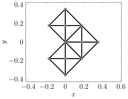 Figure 0
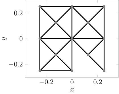 Figure 1
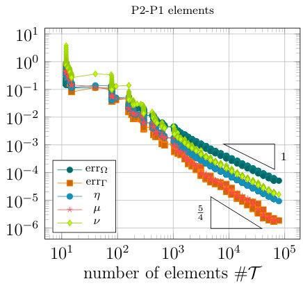 Figure 10
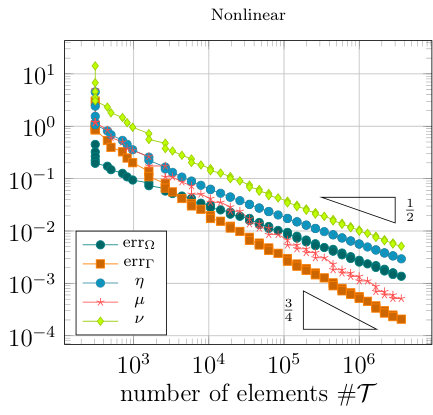 Figure 11
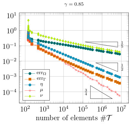 Figure 2
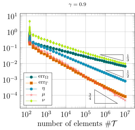 Figure 3
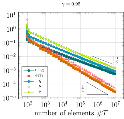 Figure 4
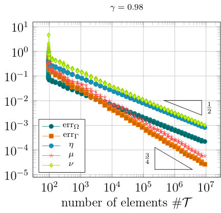 Figure 5
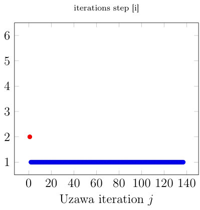 Figure 6
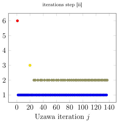 Figure 7
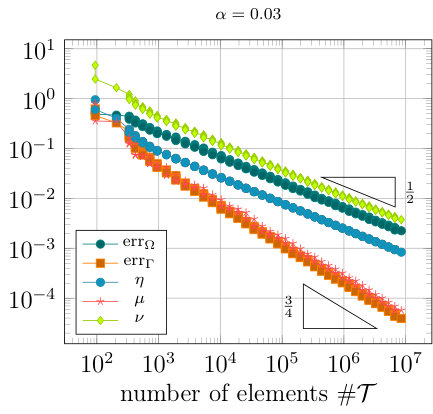 Figure 8
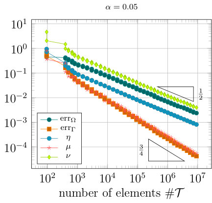 Figure 9
Peer Reviews
No public reviews on file for this paper yet. If you reviewed it on a platform where reviews are public (OpenReview, ICLR, NeurIPS, ICML), you can paste yours below so the community can read it here.
Videos
No videos yet. Explain this paper in a talk, walkthrough, or lecture? Add one.
A linear Uzawa-type solver
for nonlinear transmission problems
Thomas Führer
and
Dirk Praetorius
TU Wien, Institute for Analysis and Scientific Computing, Wiedner Hauptstr. 8–10/E101/4, 1040 Wien, Austria
[email protected] (corresponding author)
Abstract.
We propose an Uzawa-type iteration for the Johnson–Nédélec formulation of a Laplace-type transmission problem with possible (strongly monotone) nonlinearity in the interior domain. In each step, we sequentially solve one BEM for the weakly-singular integral equation associated with the Laplace-operator and one FEM for the linear Yukawa equation. In particular, the nonlinearity is only evaluated to build the right-hand side of the Yukawa equation. We prove that the proposed method leads to linear convergence with respect to the number of Uzawa iterations. Moreover, while the current analysis of a direct FEM-BEM discretization of the Johnson–Nédélec formulation requires some restrictions on the ellipticity (resp. strong monotonicity constant) in the interior domain, our Uzawa-type solver avoids such assumptions.
Key words and phrases:
FEM-BEM coupling, adaptivity, Uzawa algorithm
2010 Mathematics Subject Classification:
65N30,65N38
Acknowledgement. The authors acknowledge support through the Austrian Science Fund (FWF) under grant P27005 Optimal adaptivity for BEM and FEM-BEM coupling.
1. Introduction
1.1. State of the art
The mathematical understanding of convergence of adaptive algorithms even with optimal rates has matured. We refer to the seminal works [16, 31, 38, 13, 20] for the adaptive finite element method (FEM), [23, 25] for the adaptive boundary element method (BEM), as well as to [9] for some abstract axiomatic framework. Convergence of the adaptive FEM-BEM coupling has been proved in [5] for heuristic type error estimators as well as in [4] for residual error estimators, while the proof of optimal convergence rates is still missing due to the lack of some crucial orthogonality property (which is so far only known for elliptic problems which are symmetric up to a compact perturbation; see [20, 7]). For linear problems, the influence of the inexact (iterative) solution of the Galerkin systems on the (optimal) convergence of adaptive FEM is analyzed in [2, 20], while adaptive inexact FEM for strongly monotone problems has been considered in [24].
In the present work, we consider a possibly nonlinear transmission problem on the full space , . Then, the FEM-BEM coupling is often the method of choice, since it allows to handle the nonlinearity in the bounded FEM domain, while properly treating the radiation condition at infinity. We follow an idea from [6] for the linear Stokes problem and transfer their approach to the nonlinear FEM-BEM coupling. Unlike [24], we do not use a Picard iteration to linearize the coupled system, but employ an Uzawa-type outer iteration combined with adaptive mesh-refinement for both the FEM part and the BEM part of the coupled system in an inner iteration. One particular benefit of the proposed approach is that each step of the Uzawa iteration only considers either a linear and symmetric FEM problem or a linear BEM problem, despite the nonlinearity (or the non-symmetry) of the transmission problem resp. of its FEM-BEM coupling formulation. Moreover, our analysis of the proposed algorithm also allows the inexact (iterative) solution of these FEM or BEM problems. In particular, we employ only standard preconditioning techniques for the FEM or the BEM on adaptively refined meshes, while no preconditioner for the coupled FEM-BEM system is required.
Throughout, our focus is on the Johnson-Nédélec FEM-BEM coupling formulation [29]. Unlike the so-called symmetric coupling [28, 14] which involves all four boundary integral integral operators associated with the partial differential equation in the exterior domain, the Johnson-Nédélec coupling relies only on the simple-layer and the double-layer integral operator and, in particular, avoids the so-called hypersingular integral operator. For this reason, the Johnson-Nédélec coupling is often preferred in practice, even if the symmetric coupling is better understand from the point of numerical analysis.
We stress that well-posedness of the Johnson-Nédélec coupling on polygonal domains has only been proved recently in the seminal work [35] for linear Laplace- and Yukawa-type transmission problems (see also [37, 32, 33] for general linear problems), while stability for nonlinear problems has been treated in [4, 18]. Throughout, the current analysis requires that the ellipticity (resp. monotonicity) in the FEM domain is sufficiently large (see [37, 32, 33, 4, 18]), since the proof of the discrete inf–sup condition (resp. discrete monotonicity estimate) essentially relies on energy arguments. Numerical experiments in [4], however, indicate that this might not be necessary in practice.
In any case, it is worth noting that the present Uzawa-type algorithm only requires well-posedness of the continuous problem. Our analysis avoids any additional assumption on the validity of the discrete inf–sup condition (resp. discrete monotonicity). In explicit terms, the proposed algorithm is proved to be stable, even if the pair of discrete FEM and BEM spaces would not yield a positive inf–sup constant and would thus be unstable for the direct solution of the Johnson-Nédélec FEM-BEM coupling. Numerical experiments give evidence for optimal convergence behavior of the proposed algorithm even if the (unknown) exact solution of the transmission problem has singularities.
1.2. Model problem
With , let be a bounded and simply connected Lipschitz domain with boundary and normal vector pointing from to the unbounded domain . Given , , and , we seek the solution of the transmission problem
[TABLE]
with some unknown constant . Here, is a (nonlinear) second-order elliptic differential operator with , , and , understood in the weak sense, i.e., ,
[TABLE]
We suppose that is strongly semi-monotone and Lipschitz continuous, i.e., there exist such that, for all , it holds that
[TABLE]
In the case , we suppose that to ensure coercivity of the weakly-singular integral operator , defined in Section 2.2. It is proved, e.g., in [4, 11] that the model problem (1) then admits a unique solution . We refer to Section 2.1 for the definition of the involved function spaces.
1.3. Contributions and outline
To develop our ideas, we first formulate the Uzawa-type iteration on the continuous level. To this end, Section 2 recalls the functional analytic setting (Section 2.1) as well as the Johnson-Nédélec formulation of the transmission problem (1) (Section 2.2). Then, Algorithm 2 formulates the Uzawa iteration and Proposition 3 proves linear convergence with respect to the number of Uzawa iterations.
Section 3 is the mathematical core of the manuscript. We discretize each step of the Uzawa iteration by conforming BEM resp. FEM with piecewise polynomials of order resp. . Algorithm 4 formulates the outer Uzawa iteration for the discretized problem, and Theorem 5 proves linear convergence. The inner iteration with adaptive FEM (resp. adaptive BEM) is the topic of Section 3.3. In the spirit of [13], we give an abstract analysis of an adaptive mesh-refining algorithm (Algorithm 9) which also allows the inexact solution of the arising linear systems by means of the preconditioned conjugate gradient method (PCG). Proposition 11 proves that the algorithm reaches any prescribed tolerance in finite computational time. Moreover, for properly chosen preconditioners, the number of CG iterations in each step of the adaptive algorithm is uniformly bounded (Remark 10). We apply this adaptive algorithm in each step of the outer Uzawa iteration for the BEM part (Section 3.4) and for the FEM part (Section 3.5), where we employ a weighted-residual error estimator for the BEM and the standard residual error estimator for the FEM. Theorem 13 resp. Theorem 16 prove that the number of adaptive mesh-refinement steps (Algorithm 9) in each step of the discrete Uzawa iteration (Algorithm 4) is generically uniformly bounded.
Numerical experiments in Section 4 give empirical evidence that the proposed algorithm does not only provide a linear solution strategy for a possibly nonlinear transmission problem (1), but also leads to optimal convergence rates with respect to the number of elements.
1.4. General notation
Throughout the results, we state all constants as well as their dependencies. To abbreviate the presentation in proofs, we write if with a constant which is clear from the context. Morever, abbreviates .
2. Continuous Uzawa iteration
2.1. Involved function spaces
For any measurable subset resp. , let denote the norm which is induced by the scalar product . Let denote the usual Sobolev space on with norm
[TABLE]
Let denote the fractional Sobolev space on the boundary with norm
[TABLE]
where denotes the trace operator.
Let resp. denote the dual spaces of resp. , where the duality pairings extend the scalar products and are hence denoted by resp. . For and , we thus have
[TABLE]
The norms on and are defined by duality, i.e.,
[TABLE]
Finally, let denote the Riesz mapping, i.e.,
[TABLE]
2.2. Johnson–Nédélec formulation of model problem
With being the fundamental solution of the Laplace operator, we consider the boundary integral operators
[TABLE]
The single-layer integral operator is an isomorphism for all . Moreover, for , it is even elliptic and symmetric, i.e., and for all . The double-layer integral operator is a bounded linear operator for all .
A common way to solve (1), is to rewrite the solution of the exterior problem (1b) with the help of the representation formula. This usually leads to equations involving boundary integral operators. Different methods are available which are equivalent on the continuous level, but lead to different discrete formulations; see, e.g., [4, 14, 15, 28, 29].
In this work, we consider the Johnson–Nédélec coupling [29] with its variational formulation: Find such that
[TABLE]
for all . It is known that (4) admits a unique solution , and is the normal derivative of the exterior solution .
With being the adjoint of the trace operator, the Johnson–Nédélec coupling can equivalently be reformulated as follows: Find such that
[TABLE]
This operator formulation provides the starting point for the following Uzawa-type iterative solvers.
Remark 1**.**
If and are conforming subspaces, it is proved in [4] that the discrete Johnson–Nédélec coupling
[TABLE]
admits a unique solution provided that and is sufficiently large. While [4] requires , one can adapt [33] to see that is sufficient to ensure that the left-hand defines a (nonlinear) discrete bijection, where denotes the contraction constant of in the -induced norm. We stress, however, that our Uzawa-type iteration does not involve any assumption on .∎
2.3. Continuous Uzawa iteration
The starting point for our analysis is the following iterative solution of the Johnson–Nédélec formulation (5). We stress that each step of the algorithm requires only the solution of two linear equations.
Algorithm 2**.**
**Input: Let and .
Uzawa iteration: For all , iterate the following steps **[i]–[iii]:
- [i]
Solve for .
- [ii]
Solve for .
- [iii]
Define .
Output: Sequence in .
Proposition 3**.**
Suppose that is sufficiently small. Then, for an arbitrary initial guess , the sequence from Algorithm 2 converges linearly to the solution of the Johnson–Nédélec formulation (5), i.e., there exist and such that, for all and all it holds that
[TABLE]
Proof.
The proof is split into four steps.
Step 1. Recall from (5) that . From the mapping properties of , , and , it follows that
[TABLE]
for all . This proves the first estimate of (7).
Step 2. To prove the second estimate of (7), recall from (5) that . Hence,
[TABLE]
With and , it follows that
[TABLE]
Together with , this proves
[TABLE]
Hence, it only remains to prove that the operator is a contraction.
Step 3. We show that the operator is strongly monotone and Lipschitz continuous, i.e., there exist such that, for all ,
[TABLE]
First, Lipschitz continuity follows from Lipschitz continuity of and boundedness of the trace operator and the boundary integral operators , . Second, using the hypersingular integral operator , one can prove the identity
[TABLE]
see, e.g., [36, Section 6.6]. This so-called exterior Steklov-Poincaré operator is elliptic [11, Lemma 4] in . Together with strong semi-monotonicity of , we see
[TABLE]
for all . Since the left-hand side defines an equivalent norm on , this proves strong monotonicity of .
Step 4. We finally show that the operator is a contraction: Let . Let . Then,
[TABLE]
By choice of , it holds that . In particular, it follows from (8) that , and an induction argument concludes (7). ∎
3. Discrete Uzawa iteration
3.1. Triangulation and mesh-refinement
Throughout, we assume that is a conforming triangulation of into compact non-degenerate simplices (of dimension ). By , we denote the induced conforming triangulation of into plane non-degenerate surface simplices (of dimension ). For a simplex , let denote its -dimensional volume and let be the Euclidean diameter. The triangulation is -shape regular if
[TABLE]
Note that this implies for all . Note that -shape regularity of implies also the -shape regularity of in the sense of for all facets , where denotes the -dimensional surface area.
We suppose a fixed refinement strategy , where is the coarsest refinement of such that all marked elements have been refined, i.e., . We suppose that
- •
each element is the union of its sons, i.e., ;
- •
there exists such that for all and all with , i.e., sons are uniformly smaller than their fathers.
We write , if there exist , triangulations , and marked elements such that , for all , and . In particular, it holds that . Finally, we suppose that guarantees uniform -shape regularity, i.e., all are -shape regular (9), where depends only on .
One possible choice for is newest vertex bisection [30, 39], where .
3.2. Discrete Uzawa iteration
The discrete Uzawa iteration approximates and , where for all . To formulate the basic idea,
- •
let solve ,
- •
let solve ;
see also Algorithm 2 with the corresponding definition of resp. . With this notation, a discrete discrete Uzawa iteration reads as follows, where the precise computation of in step [i] and in step [ii] is the topic of Section 3.3–3.5.
Algorithm 4**.**
**Input: Parameter , initial triangulation , initial guess , constants and .
Discrete Uzawa iteration: For all , iterate the following steps **[i]–[iii]:
- [i]
Determine as well as some such that
[TABLE]
- [ii]
Determine a triangulation and some such that
[TABLE]
- [iii]
Define and .
The following theorem together with the realization of step [i] and step [ii] which are presented below, is the main result of the present work.
Theorem 5**.**
Suppose that is sufficiently small in the sense of Proposition 3. Let as well as . Let be an arbitrary triangulation of . Then, for an arbitrary discrete initial guess , the sequence from Algorithm 4 converges to the solution of the Johnson–Nédélec formulation (5), and it holds
[TABLE]
where and depend only on , , , and . Moreover, if is the contraction constant from Proposition 3 and , then .
Proof.
Recall from (5) that . Therefore, it follows that
[TABLE]
With and , it holds that
[TABLE]
The combination of these two observations yields
[TABLE]
Together with , we hence obtain that
[TABLE]
As in the proof of Proposition 3, it holds that
[TABLE]
Since is an isometry and , it follows that for the operator norm. Together with (10)–(11), we obtain that
[TABLE]
Let . Arguing by induction on , we prove that
[TABLE]
Note that , where the hidden constant depends only on and . This concludes convergence (12) for the FEM part, i.e., .
If , it holds that
[TABLE]
Using this estimate in (13), we prove convergence (12) for the FEM part with .
The mapping properties of the boundary integral operators reveal that
[TABLE]
Together with (10)–(11), we obtain that
[TABLE]
Therefore, convergence (12) for the BEM part follows from the above arguments. ∎
3.3. Adaptivity with inexact PCG solver
We will realize step [i] and step [ii] of Algorithm 4 by adaptive mesh-refining strategies which also include the use of the preconditioned conjugate gradient method (PCG). To this end, we follow [9] and note that step [i] and step [ii] can be covered simultaneously within the following abstract framework.
Let be a Hilbert space with scalar product and corresponding norm . For each triangulation , let be an associated discrete subspace of . We suppose that implies nestedness . For given , let be the exact solution of for all . For some fixed , let be the best approximation of in , i.e., solves
[TABLE]
or equivalently
[TABLE]
Note that this also yields the Pythagoras theorem
[TABLE]
For each and all , we suppose some refinement indicator . We define the corresponding error estimator
[TABLE]
We suppose that there are constants and such that for all and all as well as all and , the following properties (A1)–(A3) are satisfied:
- (A1)
Stability on non-refined elements: . 2. (A2)
Reduction on refined elements: . 3. (A3)
Reliability for exact best approximation: .
Let denote a basis of . Then, (14) is equivalent to solving
[TABLE]
in the sense that . Since is symmetric and positive definite, we use PCG as inexact solver and replace the exact solution by some PCG iteration, see [34, 27]. To this end, we consider
[TABLE]
instead of (18), where is a symmetric and positive definite matrix which is spectrally equivalent to , i.e.,
[TABLE]
We suppose that the constants are independent of and call an optimal preconditioner for . Then,
[TABLE]
where depends only on and , but is independent of . We refer to [42, 41, 22, 21] for optimal preconditioners for FEM and BEM on locally refined meshes.
Lemma 6** ([27, Section 11.3 and 11.5]).**
Let and with . For , let be the approximate solution of (19) after iterations of the PCG algorithm [27, Algorithm 11.5.1] with matrix , optimal preconditioner , initial guess , and right-hand side . Let be the corresponding discrete function. Then,
[TABLE]
In particular, given a tolerance , there exists a constant such that
[TABLE]
The constant depends only on , from (20) as well as on , but is independent of .∎
The proof of the following proposition follows the ideas of [13], but (unlike [13]) allows that results from the inexact solution of (15) with, e.g., PCG.
Lemma 7**.**
Let and suppose that satisfies, for some , the Dörfler marking criterion
[TABLE]
Let . Then, there exist such that the following assertion holds: If is close to the exact best approximation in the sense of
[TABLE]
then it follows that the so-called quasi-error is contractive, i.e.,
[TABLE]
The constants , depend only on , , , , and .
Proof.
Applying the Pythagoras theorem (16) twice and using (23), we prove that
[TABLE]
In addition, we may also employ reliability (A3) and stability (A1) to prove that
[TABLE]
Let which will be fixed later. Define . Then, the last two estimates lead to
[TABLE]
Having bounded the energy error, we consider the estimator. For all , it holds that
[TABLE]
Moreover, stability (A1), reduction (A2), and Dörfler marking (22) yield that
[TABLE]
We set and . Combining the last two estimates, we obtain that
[TABLE]
Let which is fixed later. Combining (26)–(27), we infer that
[TABLE]
It remains to choose . First, choose sufficiently small such that . Then, choose sufficiently small such that . Finally, choose such that
- •
q^{\prime\prime}:=\big{\{}(1+\kappa_{\rm ctr}^{-1}2\delta C_{\rm rel}^{2})(1+\varepsilon)q^{\prime}\big{\}}<1,
- •
\big{\{}(1-\delta)(1-\lambda)-C^{\prime\prime}\delta\lambda-(\kappa_{\rm ctr}+2\delta C_{\rm rel}^{2})C^{\prime}(1+\varepsilon^{-1})\big{\}}\geq 0.
This leads to
[TABLE]
and hence concludes the proof. ∎
Remark 8**.**
Note that (25) shows that
[TABLE]
where the hidden constants depend only on . The error term can efficiently be evaluated in an equivalent norm: Let be the coefficent vectors of resp. , be the stiffness matrix of , and be an optimal preconditioner. Then,
[TABLE]
where the hidden constants depend only on from (20). Note that is evaluated in each iteration of the PCG algorithm; see [27, Algorithm 11.5.1]. Therefore, no extra computational cost is needed.∎
Algorithm 9**.**
**Input: Parameter as well as , initial triangulation , initial guess , as well as tolerance .
Adaptive loop: For all , iterate the following steps **(i)–(iii), until
[TABLE]
where is defined in (29):
- (i)
Compute an approximate solution to (14), where is the minimal number such that the -th iterate in PCG with initial guess (see Proposition 6) satisfies
[TABLE]
- (ii)
Determine a set of marked elements such that
[TABLE]
- (iii)
Generate new triangulation .
Output: Smallest index , adaptively refined triangulation , and discrete approximation which satisfies the stopping criterion (30).
Remark 10**.**
Proposition 6 proves that for fixed , the smallest number of PCG iterations such that (31) holds, is uniformly bounded by some that depends only on and , but not on . For the particular choice , the condition (31) isa already satisfied after one PCG step.
Proposition 11**.**
Let , and . Then, Algorithm 9 terminates after finitely many iterations and provides some triangulation together with some discrete approximation to such that
[TABLE]
where depends only on and .
Proof.
Since marked elements are refined, i.e., , the marking criterion (32) ensures that (22) is satisfied in each step of the adaptive loop. For , the accuracy criterion (31) coincides with (23). Hence, Proposition 7 applies and provides with (24). In particular, this guarantees
[TABLE]
In particular (and formally for ), this proves as . Since , this also shows . Hence, there exists a minimal such that the stopping criterion (30) is satisfied and Algorithm 9 terminates. Remark 8 provides some constant which depends only on and , such that
[TABLE]
This concludes the proof. ∎
3.4. Realization of step [i] of Uzawa iteration
Step [i] of Algorithm 4 will be realized by means of Algorithm 9, where
[TABLE]
We employ the weighted-residual error estimator from [12, 8, 10]. We note, however, that the residual involves the integration of which can hardly be performed for continuous data . Therefore, we follow [17], suppose additional regularity , and approximate . This additional approximation error is also included in the a posteriori error estimator. Let denote the surface gradient. Recall that . Then, the overall estimator reads
[TABLE]
where denotes the -orthogonal projection onto .
Lemma 12** ([17, Proposition 2] and [17, Section 6]).**
Suppose that the discretization of is obtained
- •
either by the Scott-Zhang projection **[17]** onto for and ,
- •
or by the -orthogonal projection onto for and ,
- •
or by the -orthogonal projection onto for and , if this is -stable (see **[30, 26]**),
- •
or by nodal interpolation for and .
Suppose that releies on newest vertex bisection [30, 39] for . Then, the error estimator satisfies the assumptions (A1)–(A3) from Section 3.3, where , , and depend only on the mesh-refinement strategy and -shape regularity of . Moreover, in all these cases, implies that
[TABLE]
for all , where depends only on , , and -shape regularity of as well as the use of newest vertex bisection for . ∎
Because of Lemma 12, we can employ Algorithm 9 to realize step [i] of Algorithm 4. In particular, the following theorem proves that the number of adaptive iterations of Algorithm 9 is uniformly bounded.
Theorem 13**.**
Let , , and . For , choose and . Then, the following assertions (a)–(b) hold:
(a)* After iterations, Algorithm 9 returns the triangulation and a corresponding discrete function such that*
[TABLE]
where depends only on , , and .
(b)* Suppose that is sufficiently small in the sense of Proposition 3 and that is the resulting contraction constant of the continuous Uzawa iteration. Suppose . Moreover, suppose that there exists such that for all , the initial guess for Algorithm 9 satisfies*
[TABLE]
where is the best approximation of in with respect to . Then, the number of iterations in Algorithm 9 is uniformly bounded for all , i.e., , where depends only on , , , , , as well as on uniform -shape regularity of the triangulation and on .
Remark 14**.**
Note that (36) allows the choice . However, in our implementation, we obtain by one CG iteration with initial value . Then, depends only on the norm equivalence and hence on .∎
Proof of Theorem 13.
To prove (a), note the norm equivalence for all . The first claim together with the estimate (35) follows from Proposition 11, where with hidden norm equivalence constants.
To prove (b), note that the number of iterations is finite for . Without loss of generality, we may hence suppose . Let be the -th adaptive mesh in Algorithm 9 (in the -th iteration of Algorithm 4). Let be the corresponding approximation. Recall that Algorithm 9 guarantees that
[TABLE]
This proves that
[TABLE]
To conclude the proof of (b), it only remains to show that
[TABLE]
where is independent of . For sufficiently large (which does not depend on ) and , the stopping criterion (30) is then satisfied and hence Algorithm 9 terminates for some .
For the ease of presentation, we suppose so that all estimates hold up to norm equivalence constants (which, however, depend only on ). The proof of (37) is split into several steps.
Step 1. Recall that . For , let be the best approximation of in with respect to . Then, the triangle inequality and elementary properties of the orthogonal projection prove that
[TABLE]
and
[TABLE]
Combining these two estimates, we see that
[TABLE]
With stability of and , Proposition 5 (where is used) proves that
[TABLE]
The hidden constants depend only on , , , , and . Overall, we thus obtain that
[TABLE]
where the hidden constant depends only on , , , , , and .
Step 2a. Since Algorithm 9 terminated in the -th iteration, the stopping criterion (30) with implies that . To simplify notation, let be the local mesh-size, . Recall that and that is associated with . Since , this proves that
[TABLE]
Step 2b. We employ the local inverse estimate for from [3] to see that
[TABLE]
As in Step 1, the first term is estimated by The second term is estimated with (34) as Altogether, we obtain
[TABLE]
where the hidden constant depends only on , , , , , , , and -shape regularity of .
Step 2c. We employ the local inverse estimate for from [3] to see that
[TABLE]
As in Step 1, it holds that
[TABLE]
where the hidden constant depends only on , , , , , -shape regularity of , the polynomial degree , and on .
Step 2d. Recall that . The combination of Step 2a–2c proves
[TABLE]
Overall, the combination of Step 1 and Step 2d verifies (37) and hence concludes the proof.
∎
3.5. Realization of step [ii] of Uzawa iteration
Step [ii] of Algorithm 4 will be realized by means of Algorithm 9, where
[TABLE]
Note that . We employ a weighted-residual error estimator similar to, e.g., [1, 40]. We suppose additional regularity . Recall that . Therefore, the estimator reads
[TABLE]
The following observation goes back to [13], where the properties (A1)–(A2) are implicitly proved in [13, Section 3.1].
Lemma 15**.**
The error estimator satisfies the assumptions (A1)–(A3) from Section 3.3, where , , and depend only on the mesh-refinement strategy and -shape regularity of .
Sketch of proof.
Throughout, we suppose that and . To see (A1), let and , . Then,
[TABLE]
Together with an inverse inequality and the trace inequality, we hence obtain that
[TABLE]
The constant depends only on the mesh-refinement strategy , -shape regularity of , and the polynomial degree .
To see (A2), note that all local contributions to the estimator are weighted with either or . Therefore, (A2) simply follows from reduction of refined elements; see Section 3.1.
Finally, reliability (A3) follows with the same techniques as in [1, 40]. The only difference is that we have to tackle the term from the right-hand side. In general, this term is not in . However, elementwise integration by parts proves
[TABLE]
for all . With this identity, the residual can be estimated with standard techniques. ∎
Because of Lemma 15, we can employ Algorithm 9 to realize step [ii] of Algorithm 4. Moreover, provided that the inverse-type inequality
[TABLE]
holds for all with some hidden constant that depends only on , , , the polynomial degree , and -shape regularity of , the following theorem proves that the number of adaptive iterations of Algorithm 9 is uniformly bounded.
Theorem 16**.**
Let , , and . For , choose and . Then, the following assertions (a)–(b) hold:
(a)* After iterations, Algorithm 9 returns the triangulation and a corresponding discrete function such that*
[TABLE]
where depends only on , , and .
(b)* Suppose that is sufficiently small in the sense of Proposition 3 and that ist the resulting contraction constant of the continuous Uzawa iteration. Suppose . Moreover, suppose that there exists such that for all , the initial guess for Algorithm 9 satisfies*
[TABLE]
where is the best approximation of in with respect to . Finally, suppose that (3.5) holds. Then, the number of iterations in Algorithm 9 is uniformly bounded for all , i.e., , where depends only on , , , , , as well as on uniform -shape regularity of the triangulation and on .
Remark 17**.**
We note that the additional assumption (3.5) on is satisfied if is linear with coefficients , , and .
Proof of Theorem 16.
To prove (a), note that for all . The first claim together with estimate (39) follows from Proposition 11, where .
To prove (b), we argue as in the proof of Proposition 13. We may suppose . Let be the -th adaptive mesh in Algorithm 9 (in the -th iteration of Algorithm 4). Let be the corresponding approximation. Recall that Algorithm 9 guarantees that
[TABLE]
To conclude the proof of (b), it only remains to show that
[TABLE]
where is independent of .
Step 1. Lipschitz continuity of , the definitions of the dual norms , , and Proposition 5 (where ) prove that
[TABLE]
The hidden constants depend only on , , , , and . Arguing as in step 1 of the proof of Proposition 13, we conclude .
Step 2. As above, the stopping criterion (30) implies that . Following the proof of Proposition 13, we obtain that
[TABLE]
with
[TABLE]
Note that and . Together with an inverse inequality and the assumption (3.5), this proves that
[TABLE]
Hence,
[TABLE]
This finishes the proof. ∎
3.6. Global a posteriori error estimate
In this section, we derive a global upper bound for the error . To that end, let
[TABLE]
denote the operator associated to the Johnson-Nédélec coupling (4). Let be the best approximation of with respect to and let be the best approximation of with respect to the induced norm. The upper bound in the next theorem involves the terms
[TABLE]
which stem from the fact that we use inexact solvers. In our setting, these terms are evaluated within the PCG algorithm and hence known a posteriori terms; see Remark 8.
Theorem 18**.**
Suppose that is
- •
either linear with
- •
or strongly monotone with ,
where denotes the contraction constant of the double-layer integral operator. Then, there holds
[TABLE]
The constant depends only on , , , , , -shape regularity of , and .
Proof.
Define and let denote the duality pairing between and its dual . We stress that exists and is Lipschitz continuous, i.e.,
[TABLE]
To see (42) in the case that is strongly monotone with , one follows [19, Section 5.1]. If is linear with , the Johnson-Nédélec coupling (4) is equivalent to the model problem (1). Note that is bijective, so that the right-hand side in (4) is an arbitrary functional on . Therefore, unique solvability of the model problem (1) proves that is bijective. The inverse mapping theorem thus implies (42).
Recall the Richardson iteration in the Uzawa algorithm. Therefore,
[TABLE]
Lipschitz continuity of shows that
[TABLE]
To estimate the boundary contribution, recall that and . Together with Remark 8, this proves that
[TABLE]
To estimate the volume contribution, recall that and . This gives
[TABLE]
With the triangle inequality and Remark 8, we further infer that
[TABLE]
Putting all together, we conclude the proof. ∎
4. Numerical examples
In this section, we present three numerical experiments in 2D to underpin our theoretical findings. We consider two linear problems on an L-shaped domain and a nonlinear problem on a Z-shaped domain, sketched in Figure 1. In all examples, the exact solution of (1) is known and the solution in the interior has a singularity at the reentrant corner. We compute the error quantities (in each step of Algorithm 4)
[TABLE]
and compare them to the error estimators and the global error estimator . Here, denotes the local mesh-size . In all convergence plots, we use triangles to visualize slopes , where the experimental convergence rate is written besides the triangle. The parameter for the Dörfler marking criterion (22) is set to .
4.1. Laplace transmission problem
We choose , where denote the polar coordinates. The exterior solution is a smooth function. We set , , . Hence, the operator simplifies to
[TABLE]
which corresponds to the case of the Laplace transmission problem. The approximation order of the spaces is set to , i.e., we use the spaces and . Figure 2 shows the error quantities, and estimators over the number of elements for a fixed and . We observe suboptimal rates , resp. for resp. , whereas lead to the optimal rate for the overall error. This indicates that the contraction constant from Proposition 5 satisfies and . Comparing the number of total iterations () in the Uzawa-type Algorithm 4, we get for . Altough in both cases we obtain optimal convergence rates, much more iterations are needed for .
For all values of , we observe that the number of iterations within the steps [i] and [ii] of Algorithm 4 is bounded, i.e., the number of BEM and FEM problems to be solved is bounded (see Theorem 13 and Theorem 16). Figure 3 visualizes the number of iterations in step [i] and step [ii] with respect to the number of iterations (indexed with ) in Algorithm 4 for . The FEM and BEM problems are solved using PCG with appropriate (local) multilevel additive Schwarz preconditioners and relative tolerance (see Section 3.3).
4.2. Modified Uzawa algorithm
The observations of the last section lead us to a modified algorithm (not analyzed), where we adapt the value of at the end of each iteration. This modification is based on the following observation, which follows along the proof of Proposition 5: It holds that
[TABLE]
and thus
[TABLE]
This proves that
[TABLE]
Since the exact iterates are not known, we replace them by our approximations in the following algorithm. Recall that .
Algorithm 19**.**
**Input: Parameter , initial triangulation , initial guess , constants , and .
Discrete Uzawa iteration: For all , iterate the following steps **[i]–[v]:
- [i]
Determine as well as some such that
[TABLE]
- [ii]
Determine a triangulation and some such that
[TABLE]
- [iii]
Define and .
- [iv]
If update .
- [v]
Set .
4.3. Laplace transmission problem with modified Algorithm
We consider the same example and configuration as in Section 4.1, but now use the modified Algorithm 19 instead of Algorithm 4. We set with initial . Figure 4 shows the error quantities and error estimators over the number of elements for and .
We observe that both values of lead to optimal rates for the overall error with respect to the number of volume elements. For , we obtain a total of iterations, which is much less in comparison to the iterations obtained in Section 4.1 with a fixed .
4.4. Transmission problem using higher order elements
We consider essentially the same setting as in Section 4.3, but now use higher order elements . We set and use an exact solver for the realization of step [i] and [ii] in Algorithm 19. Furthermore, we replace by the operator
[TABLE]
Note that for this operator there holds . We stress that it is not known whether the discrete Johnson-Nédélec coupling (6) is solvable or not; see Remark 1. Figure 5 (left plot) shows the error quantities and error estimators with respect to the number of elements. As before, we observe an optimal decay of the overall error with respect to the number of elements, which in the case is .
4.5. Nonlinear transmission problem on Z-shaped domain
We consider a nonlinear transmission problem on the Z-shaped domain sketched in Figure 1. Again we apply Algorithm 19 with , and initial . We use lowest-order elements for the approximations and an exact solver to realize step [i] and [ii] of Algorithm 19. We set and with for and , hence, reads
[TABLE]
It can be proved that is strongly monotone with constant . We prescribe the exact interior solution in polar coordinates and use a smooth function for the exterior solution . The error quantities and error estimators over the number of elements are plotted in Figure 5 (right plot). Again we observe an optimal decay of the overall error.
The reference list from the paper itself. Each links out to its DOI / PubMed record.
- 1[1] M. Ainsworth and J. T. Oden. A posteriori error estimation in finite element analysis . Pure and Applied Mathematics (New York). Wiley-Interscience [John Wiley & Sons], New York, 2000.
- 2[2] M. Arioli, E. H. Georgoulis, and D. Loghin. Stopping criteria for adaptive finite element solvers. SIAM J. Sci. Comput. , 35(3):A 1537–A 1559, 2013.
- 3[3] M. Aurada, M. Feischl, T. Führer, M. Karkulik, J. Melenk, and D. Praetorius. Local inverse estimates for non-local boundary integral operators. Math. Comp. , in print, 2017.
- 4[4] M. Aurada, M. Feischl, T. Führer, M. Karkulik, J. M. Melenk, and D. Praetorius. Classical FEM-BEM coupling methods: nonlinearities, well-posedness, and adaptivity. Comput. Mech. , 51(4):399–419, 2013.
- 5[5] M. Aurada, M. Feischl, and D. Praetorius. Convergence of some adaptive FEM-BEM coupling for elliptic but possibly nonlinear interface problems. ESAIM Math. Model. Numer. Anal. , 46(5):1147–1173, 2012.
- 6[6] E. Bänsch, P. Morin, and R. H. Nochetto. An adaptive Uzawa FEM for the Stokes problem: convergence without the inf-sup condition. SIAM J. Numer. Anal. , 40(4):1207–1229, 2002.
- 7[7] A. Bespalov, A. Haberl, and D. Praetorius. Adaptive FEM with coarse initial mesh guarantees optimal convergence rates for compactly perturbed elliptic problems. Comput. Methods Appl. Mech. Engrg. , 317:318–340, 2017.
- 8[8] C. Carstensen. An a posteriori error estimate for a first-kind integral equation. Math. Comp. , 66(217):139–155, 1997.