This paper studies the evolution of axisymmetric curves driven by mean curvature with boundary conditions in the half space, classifying solutions and analyzing fattening phenomena using level set methods.
Contribution
It introduces criteria for fattening in curvature flow with boundary conditions and classifies solution behaviors in this context.
Findings
01
Classified solutions into three categories.
02
Provided criteria to determine fattening or non-fattening.
03
Described asymptotic behaviors for each solution category.
Abstract
We consider a family of axisymmetric curves evolving by its mean curvature with driving force in the half space. We impose a boundary condition that the curves are perpendicular to the boundary for t>0, however, the initial curve intersects the boundary tangentially. In other words, the initial curve is oriented singularly. We investigate this problem by level set method and give some criteria to judge whether the interface evolution is fattening or not. In the end, we can classify the solutions into three categories and provide the asymptotic behavior in each category. Our main tools in this paper are level set method and intersection number principle.
No public reviews on file for this paper yet. If you reviewed it on a platform where reviews are public (OpenReview, ICLR, NeurIPS, ICML), you can paste yours below so the community can read it here.
Videos
No videos yet. Explain this paper in a talk, walkthrough, or lecture? Add one.
Taxonomy
TopicsAdvanced Mathematical Modeling in Engineering · Geometric Analysis and Curvature Flows · Nonlinear Partial Differential Equations
Full text
On curvature flow with driving force under Neumann boundary conditon in the plane
Longjie ZHANG
(Date: December, 2015
Corresponding author University:Graduate School of Mathematical Sciences, The University of Tokyo. Address:3-8-1 Komaba Meguro-ku Tokyo 153-8914, Japan. Email:[email protected], [email protected])
Abstract: We consider a family of axisymmetric curves evolving by its mean curvature with driving force in the half space. We impose a boundary condition that the curves are perpendicular to the boundary for t>0, however, the initial curve intersects the boundary tangentially. In other words, the initial curve is oriented singularly. We investigate this problem by level set method and give some criteria to judge whether the interface evolution is fattening or not. In the end, we can classify the solutions into three categories and provide the asymptotic behavior in each category. Our main tools in this paper are level set method and intersection number principle.
Keywords and phrases: mean curvature flow, driving force, Neumann boundary, level set method, singularity, fattening.
2010MSC: 35A01, 35A02, 35K55, 53C44.
[TABLE]
1. Introduction
This paper studies the planar curvature flow with driving force and Neumann boundary condition of the form
[TABLE]
[TABLE]
[TABLE]
where Ω={(x,y)∈R2∣x≥0}, V is the outer normal velocity of Γ(t), κ is the curvature of Γ(t) and the sign is chosen such that the problem is parabolic. A called driving force is a positive constant.
In this paper, we consider the initial curve Λ0 is closed, smooth and given by
[TABLE]
for u0(x)∈C[0,b0]∩C∞(0,b0). By the assumption of Λ0, there hold
[TABLE]
and
[TABLE]
Before giving our main results, we first consider another problem.
[TABLE]
[TABLE]
We consider this problem by level set method. Seeing the theory in [11], there exists unique viscosity solution ϕ of the following level set equation
[TABLE]
where a1(x,y) satisfies Λ0={(x,y)∣a1(x,y)=0}. The results in appendix show that the zero set of ϕ is not fattening. Indeed, thanks to Theorem 4.5, the zero set of ϕ can be written into
[TABLE]
Moreover, (v,a∗,b∗) is the solution of the following free boundary problem
[TABLE]
And a∗ and b∗ are called the end points of Λ(t).
Here we give our main results.
Theorem 1.1**.**
If there exists δ such that a∗(t)<0, for 0<t<δ, then there exist T1>0 and a unique smooth family of smooth curves Γ(t) satisfying (1.1), (1.2), 0≤t<T1, and satisfying (1.3) in the sense that t→0+limdH(Γ(t),Λ0)=0. Moreover, Γ(t) can be written into Γ(t)={(x,y)∈Ω∣∣y∣=u(x,t),0≤x≤b(t)}. And (u,b) is the unique solution of the following free boundary problem
[TABLE]
[TABLE]
[TABLE]
Here dH(A,B) denotes the Hausdorff distance defined as
[TABLE]
Let T be the maximal smooth time given by
[TABLE]
Theorem 1.2**.**
(Classification) Under the same assumptions of Theorem 1.1, denote
h(t)=0≤x≤b(t)maxu(x,t).Then Γ(t) must fulfill one of the following situations.
(1). (Expanding) The existence time T=∞ and both h(t) and b(t) tend to ∞, as t→∞.
(2). (Bounded) The existence time T=∞ and both h(t) and b(t) are bounded from above and below by two positive constants, as t→∞.
(3). (Shrinking) The existence time T<∞ and both h(t) and b(t) tend to 0, as t→T.
Theorem 1.3**.**
(Asymptotic behavior) Under the same assumptions of Theorem 1.1. Then Γ(t) must fulfill one of following three conditions.
(1). (Expanding) Assume that T=∞ and that both h(t) and b(t) tend to ∞ as t→∞, there exist t0>0, R1(t), R2(t) such that
[TABLE]
where U(t)={(x,y)∈R2∣∣y∣<u(x,t),x>0}. Moreover t→∞limR1(t)/t=t→∞limR2(t)/t=A.
(2). (Bounded) Assume that T=∞ and that both h(t) and b(t) are bounded from above and below by two positive constants for t>0. Then t→∞limdH(Γ(t),∂B1/A((0,0))∩{x≥0})=0.
(3). (Shrinking) Assume that T<∞ and that both h(t) and b(t) tend to 0 as t→T. Then the flow Γ(t) shrinks to a point at t=T.
We extend Γ(t) by even and still denote the extended curve by Γ(t). Then problem (1.1), (1.2), (1.3) is equivalent to the following problem in whole space
[TABLE]
[TABLE]
If we extends u0 by even(still denoted by u0), then obviously
[TABLE]
In this paper we consider the problem (1.7), (1.8) instead of the problem (1.1), (1.2), (1.3).
We next give a sufficient result to have a fattening phenomenon. The definition of interface evolution and fattening are given in section 2.
Theorem 1.4**.**
(Fattening)
If there exists δ such that a∗(t)≥0, for 0<t<δ, the interface evolution Γ(t) for (1.7) with initial data Γ0 is fattening.
Theorem 1.1 and Theorem 1.4 can be explained by Figure 2 and 3. φ in Figure 2 and 3 is given by the unique viscosity solution of
[TABLE]
where a2(x,y) satisfies Γ0={(x,y)∣a2(x,y)=0}. Let Γ(t)={(x,y)∣φ(x,y,t)=0}.
Remark 1.5*.*
The assumptions for a∗(t) in Theorem 1.1 and 1.4 seem not to be understood easily. Here we explain the assumptions by giving some sufficient conditions.
Denoting κ(O) as the curvature of Λ0 at origin, it is easy to see that
[TABLE]
Then we can prove that if
(a). κ(O)<A, there holds a∗(t)<0, for t small;
(b). κ(O)>A, there holds a∗(t)>0, for t small.
Since
[TABLE]
The role of a∗(t) in main theorem. Let (u,b) is the unique solution of the free boundary problem (1.4), (1.5), (1.6). Obviously, the flow Γ∗(t)={(x,y)∣∣y∣=u(x,t),0≤x≤b(t)} satisfies (1.1), (1.2), (1.3) naturally.
Let (v,a∗,b∗) be the solution of the problem (*). If a∗(t)≥0, 0<t<δ, the curves
[TABLE]
are located in {x≥0}.
Note that Γ∗(0)=Λ(0)=Λ0. However, Γ∗(t) are perpendicular to y-axis and the family {Λ(t)} evolves freely. This means that there exist two types of flows Γ∗(t) and Λ(t) evolving by V=−κ+A with the same initial curve Λ0. This can be considered as non-uniqueness. Indeed, seeing the proof of Theorem 1.4, the flow given by extending Γ∗(t) evenly is the boundary of closed evolution and the flow given by extending Λ(t) evenly is the boundary of open evolution.
If a∗(t)<0, 0<t<δ, the problem () will not make sense in the half space {x≥0}. But the solution given by () plays the role of a sub-solution (in the proof of Lemma 5.6). Using this sub-solution, the boundaries of the open evolution and closed evolution are away from the x-axis. By the uniqueness result(Proposition 5.4), we can prove they are the same.
In the curve shortening flow——A=0, since a∗(t)≥0 always holds, the interface evolution is fattening.
Motivation. This research is motivated by [18], the mean curvature flow with driving force under the Neumann boundary condition in a two-dimensional cylinder with periodically undulating boundary.
In [18], they only consider the condition that for initial curve {(x,y)∈R2∣y=u0(x)} with ∣u0′(x)∣<M for some M. They show that the interior point of Γ(t)={(x,y)∈R2∣y=u(x,t)} never touches the boundary and Γ(t) remains graph. Therefore, the problem can be studied by the classical parabolic theory. If removing the assumption ∣u0′(x)∣<M, when u(x,t) touches the boundary, the singularity will develop(Figure 5). Noting Figure 5, after touching, Γ(t) will possibly separate into two parts and become non-graph(Γ(t) can't be represented by y=u(x,t)). This makes us analyze what will happen after touching boundary. Since Γ(t) may become non-graph, we want to use the level set method established by [9]; see also Evans and Spruck [6] for the mean curvature flow, where fattening phenomenon is first observed. Therefore the main task in this paper is to study whether the interface evolution is fattening or not. The notion of the level set solution is introduced in Section 2.
A short review for mean curvature flow. For the classical mean curvature flow: A=0 in (1.1), there are many results. Concerning this problem, Huisken [15] shows that any solution that starts out as a convex, smooth, compact surface remains so until it shrinks to a "round point" and its asymptotic shape is a sphere just before it disappears. He proves this result for hypersurfaces of Rn+1 with n≥2, but Gage and Hamilton [10] show that it still holds when n=1, the curves in the plane. Gage and Hamilton also show that embedded curve remains embedded, i.e. the curve will not intersect itself. Grayson [13] proves the remarkable fact that such family must become convex eventually. Thus, any embedded curve in the plane will shrink to "round point" under curve shortening flow. But in higher dimensions it is not true. Grayson [14] also shows that there exists a smooth flow that becomes singular before shrinking to a point. His example consisted of a barbell: two spherical surfaces connected by a sufficiently thin "neck". In this example, the inward curvature of the neck is so large that it will force the neck to pinch before shrinking. In [3], A. Altschuler, S. B. Angenent and Y. Giga study the flow whose initial hypersurface is a compact, rotationally symmetric hypersurface but pinching on x-axis by level set method. They proved the hypersurface will separate into two smooth hypersurfaces after pinching.
Main method. In this paper, one of the most important tools is the intersection number principle. It was also used in [3] that the intersection number between two families evolving by mean curvature flow is non-increasing. But for the problem with driving force, their intersection number may increase. In [12], they give the extended intersection number principle for the following free boundary problem called (Q)
[TABLE]
where 0<θ±<π/2.
If (u1,a1,b1), (u2,a2,b2) are the solutions of (Q) with θ±1, θ±2, u01 and u02, the intersection number between
[TABLE]
and
[TABLE]
will increase possibly, by some simple examples(here we omit it). In [12], they find a non-increasing quantity. If u1 and u2 are extended by straight line, such that the extended functions u1∗, u2∗ are in C1(R), then the intersection number between u1∗ and u2∗ is non-increasing provided that θ±1=θ±2. If θ+1=θ+2, the intersection number will not increase provided that b1(t)=b2(t) and decrease at t0 satisfying b1(t0)=b2(t0). Similarly for a(t). These results are called ``extended intersection number principle''.
As we observing before, in this paper, the curve symmetric around x-axis is considered. Under this condition, θ± in problem (Q) satisfy θ±=π/2. If we extend u1 and u2 by vertical straight line, it will be seen that the extended C1 curve γ1(t) and γ2(t)(Since θ±=π/2, the extended curve will not be graph) will intersect with each other even if the intersection number between γ1(0) and γ2(0) is zero. We will investigate the intersection number in Section 4.
The rest of this paper is organized as follows. In Section 2, we introduce the level set method established by [9]. The definition of open evolution, closed evolution, fattening and the basic knowledge including comparison principle, monotone convergence theorem and so on are given in this section. In Section 3, we prove the Evans-Spruck estimate(also called gradient interior estimate). In Section 4, the results of intersection number are investigated and their application are given. In Section 5, we give the proof of Theorem 1.1 and Theorem 1.4. In Section 6, we study the possible formations of singularity. In Section 7, we classify the solution given by Theorem 1.1 and prove the asymptotic behavior in each category(Theorem 1.2 and 1.3). In Section 8, we give another non-fattening result in (n+1)-dimension with a type of initial hypersurfaces.
2. Level set method
Since the initial curve Γ0 given in (1.8) has singularity at (0,0), the equation V=−κ+A does not make sense at t=0. Therefore, we want to apply the level set method to our problem. In this section, we introduce the level set method in RN. For Γ(t) being a smooth family of smooth, closed, compact hypersurfaces in RN. Assume there exists ψ(x,t) such that Γ(t)={x∣ψ(x,t)=0,x∈RN}. If Γ(t) evolves by (1.7), we can derive ψ(x,t) satisfying
[TABLE]
Equation (2.1) is called the level set equation of (1.7). Theorem 4.3.1 in [11] gives the existence and uniqueness of the viscosity solution for (2.1) with ψ(x,0)=ψ0(x). Where ψ0(x) is a bounded and uniform continuous function.
Level set method Using the solution of level set equation, we introduce the level set method.
Definition 2.1**.**
(1) Let D0 be a bounded open set in RN. A family of open sets {D(t)∣D(t)⊂RN}0<t<T is called an (generlized)openevolution of (1.7) with initial data D0 if there exists a viscosity solution ψ of (2.1) that satisfies
[TABLE]
(2) Let E0 be a bounded closed set in RN. A family of closed sets {E(t)∣E(t)⊂RN}0<t<T is called a (generlized)closedevolution of (1.7) with initial data E0 if there exists a viscosity solution ψ of (2.1) that satisfies
[TABLE]
The set Γ(t)=E(t)∖D(t) is called an (generalized) interface evolution of (1.7) with initial data Γ0=E0∖D0.
Remark 2.2*.*
(1) For open set D0, we often choose
[TABLE]
where
[TABLE]
(2) Seeing that the choice of ψ(x,0) isn't unique, but by the Theorem 4.2.8 in [11], the open evolution D(t) and closed evolution E(t) are both independent on the choice of ψ(x,0).
(3) In generally, even if E0=D0, we can not guarantee E(t)=D(t). If E(t)∖D(t) has interior points for some t, we call the interface evolution is fattening. Respectively, if E(t)=D(t), for all 0<t<T, we say the interface evolution is regular. Therefore, in the proof of Theorem 1.1, it is sufficient to prove ∂D(t)=∂E(t). In the proof of Theorem 1.4, it is sufficient to prove that there exists a ball B such that B⊂E(t)∖D(t).
We now list some fundamental properties of open evolution and closed evolution of (1.7)(Chapter 4 in [11]).
Theorem 2.3**.**
(Semigroups)[11]. Denote U(t) and M(t) being the operators such that
U(t)D0=D(t) and M(t)E0=E(t), for t>0. Then we have U(t)D(s)=D(t+s) and M(t)E(s)=E(t+s), for any t>0, s>0.
Theorem 2.4**.**
(Order preserving property)[11]. Let D0, D0′ be two open sets in RN and let E0, E0′ be two closed sets in RN. Then
(1) U(t)D0⊂U(t)D0′, if D0⊂D0′;
(2) M(t)E0⊂M(t)E0′, if E0⊂E0′;
(3) U(t)D0⊂M(t)E0′, if D0⊂E0′;
(4) E0⊂D0 and dist(E0,∂D0)>0, then M(t)E0⊂U(t)D0.
(1) Let D(t) and {Dj(t)} be open evolutions with initial data D0 and Dj0 respectively. If Dj0↑D0, then Dj(t)↑D(t), t>0, i.e., j≥1⋃Dj(t)=D(t);
(2) Let E(t) and {Ej(t)} be closed evolutions with initial data E0 and Ej0 respectively. If Ej0↓E0, then Ej(t)↓E(t), t>0, i.e., j≥1⋂Ej(t)=E(t).
Theorem 2.6**.**
(Continuity in time)[11]. Let D(t) and E(t) be open and closed evolutions, respectively.
(1a) D(t) is a lower semicontinuous function of t∈[0,T), in the sense that for any t0≥0, and sequence xn∈(D(tn))c with xn→x0, tn→t0, the limit x0∈(D(t0))c. If D(0) is bounded so that Cϵ(D(t0)) is compact, this implies that for any t0≥0, ϵ>0 there is a δ>0 such that ∣t−t0∣<δ implies D(t)⊃Cϵ(D(t0)).
(1b) E(t) is an upper semicontinuous function of t∈[0,T), in the sense that for any t0≥0, and sequence xn∈E(tn) with xn→x0, tn→t0, the limit x0∈E(t0). If E(0) is bounded so that Nϵ(E(t0)) is compact, this implies that for any t0≥0, ϵ>0 there is a δ>0 such that ∣t−t0∣<δ implies E(t)⊂Nϵ(E(t0)).
(2a) D(t) is a left upper semicontinuous in t in the sense that for any t0∈(0,T), x0∈(D(t0))c there is a sequence xn→x0 and tn↑t0 with xn∈(D(tn))c. Moreover, for any t0∈(0,T), ϵ>0 there exists a δ>0 such that t0−δ<t<t0 implies Cϵ(D(t))⊂D(t0).
(2b) E(t) is a left lower semicontinuous in t in the sense that for any t0∈(0,T), x0∈E(t0) there is a sequence xn→x0 and tn↑t0 with xn∈E(t0). Moreover, for any t0∈(0,T), ϵ>0 there exists a δ>0 such that t0−δ<t<t0 implies Nϵ(E(t))⊃E(t0).
Where Nϵ(A)={x∈RN∣d(x,A)<ϵ}, for A is a closed subset in RN and Cϵ(A)=Nϵ(Ac)c, for A is an open subset in RN.
Remark 2.7*.*
For A>0, even if D1(0) and D2(0) are disjoint, D1(t) and D2(t) may intersect. The basic reason is that the level set equation (2.1) is not orientation free(If u is a solution, there does not hold that −u is also a solution for (2.1)).
In order to prove Theorem 1.4, we need the following lemma. This lemma gives the construction of an open evolution containing two disjoint components.
Lemma 2.8**.**
Assume D1(t) and D2(t) being the open evolution of (2.1) with D1(0)=U1 and D2(0)=U2. And D(t) is denoted as the open evolution of (2.1) with D(0)=U1∪U2. If D1(t)∩D2(t)=∅ for 0≤t≤T, then D(t)=D1(t)∪D2(t), 0≤t≤T.
Under the condition A=0, D1(t)∩D2(t)=∅ holds automatically provided that D1(0)∩D2(0)=∅. But for A>0, it is not true. Therefore, we give the assumption D1(t)∩D2(t)=∅ for 0≤t≤T.
Proof.
First, we assume D1(t)∩D2(t)=∅ for 0≤t≤T and δ=:0≤t≤Tmindist(D1(t),D2(t))>0. We define
[TABLE]
In the theory in [11], there exist non-negative φi(x,t)∈Cc(RN×[0,T]) being the solution of (2.1) with φi(x,0)=ai(x). Then Di(t)={x∈RN∣φi(x,t)>0} and φi=0 hold outside of Di(t), i=1,2. Since suppφ1 and suppφ2 are seperated by δ, it is easy to show that φ(x,t)=:max{φ1,φ2}(x,t) is also a viscosity solution of (2.1). Then D(t)={x∣φ(x,t)>0}=D1(t)∪D2(t) with initial data D(0)=U1∪U2, for 0≤t≤T.
Next we prove the result only under the assumption D1(t)∩D2(t)=∅, 0≤t≤T. Consider Dij(t)={x∣φi(x,t)>j1}.
We claim that 0≤t≤Tmindist(D1j(t),D2j(t))>0, for all j. If 0≤t≤Tmindist(D1j(t),D2j(t))=0, for some j, then there exist t0∈[0,T] and sequences {xm}⊂D1j(t0), {ym}⊂D2j(t0) such that
[TABLE]
Then there exists x, such that m→∞limxm=m→∞limym=x. Then
[TABLE]
Consequently, x∈D1(t0)∩D2(t0)=∅, contradiction. Then we have 0≤t≤Tmindist(D1j(t),D2j(t))>0, for all j. By the argument in the first step, there holds Dj(t)=D1j(t)∪D2j(t) is the open evolution with initial openset {x∣φ1(x,0)>j1}∪{x∣φ2(x,0)>j1}, for 0≤t≤T.
Noting j=1⋃∞D1j(0)∪D2j(0)=U1∪U2 and using Theorem 2.5, D(t)=j=1⋃∞Dj(t)=j=1⋃∞D1j(t)∪D2j(t)=D1(t)∪D2(t), for 0≤t≤T.
∎
Theorem 2.9**.**
(Relation between evolution and mean curvature flow) Let D(t), E(t) be the open evolution and closed evolution, respectively. Assume that in an open region U×(t1,t2)⊂RN×(0,T), ∂D(t) and ∂E(t) are the graph of continuous functions v1, v2. Precisely,
[TABLE]
and
[TABLE]
where x′=(x1,⋯,xN−1), U′=U∩{xN=0} and v1, v2 are continuous in U′×(t1,t2). Then the function v1(v2) is a viscosity supersolution(subsolution) of
[TABLE]
or is a viscosity subsolution(supersolution) of
[TABLE]
where the signs of the last terms are determined by the direction of the normal velocity of ∂D(t)∩U and ∂E(t)∩U.
We can use the similar method in [8] to prove this theorem. Here we omit it.
3. A Priori estimates
In this section, we give an interior gradient estimate.
Graph equation Let u(x,t) be some function on an open subset of Rn×R, then the graph of u(x,t) is a family of hypersurfaces in Rn+1. If the family of hypersurfaces moves by V=−κ+A if and only if
[TABLE]
where the signs of the last terms are determined by direction of the normal velocity V.
Under the case A=0,
[TABLE]
The estimate for ∣∇u∣ in entire space Rn is given by [5]. The interior estimate of gradient is first given by [8]. Here we give the estimate under the condition A>0. Since the proof for n=1 is not easier than n≥2, we prove it in n-dimensional setting.
Theorem 3.1**.**
For u∈C3(ΩT)∩C0(ΩT), u satisfies
[TABLE]
For the condition $+$''(−''), we assume u<0(u>0) in ΩT, u(0,T)=−v0(u(0,T)=v0). Then
[TABLE]
where K=20v02(4n+T1+4A+2v0A)+2, ΩT=B1(0)×(0,2T) and
[TABLE]
Proof.
We only prove the condition "+". For the condition, we can consider ``−u'' to get the result. Denote w=1+∣∇u∣2, νi=uxi/1+∣∇u∣2, gij=δij−νiνj. We define the operator L as
[TABLE]
We let h=η(x,t,u(x,t))w, where η is a non-negative function and will be identified in future. By calculation,
[TABLE]
Then
[TABLE]
We claim that
[TABLE]
Therefore, there holds
[TABLE]
We begin to prove the claim. Seeing
[TABLE]
we have
[TABLE]
[TABLE]
Combining
[TABLE]
[TABLE]
Therefore
[TABLE]
Then
[TABLE]
We complete the proof of the claim.
Next we choose η=f∘ϕ(x,t,u(x,t)),
[TABLE]
and
[TABLE]
When ϕ>0, there holds
[TABLE]
Consequently, when ϕ>0, z<0, 0<t<2T,
[TABLE]
By calculation,
[TABLE]
[TABLE]
Combining
[TABLE]
there holds
[TABLE]
When ∣∇u∣≥max{16v0,2}, we have
[TABLE]
Then
[TABLE]
when we choose K=20v02(4n+T1+4A+2v0A)+2, ΩT=B1(0)×(0,2T).
(1) In Theorem 3.1, ΩT can be replaced by ΩT=BR(x0)×(0,2T) and v0=u(x0,T). Then the conclusion becomes
[TABLE]
where K=20R2v02(4n+TR2+R4A+2v0A)+2. We can set v(x,t)=Ru(Rx+x0,R2t), then we can use Theorem 3.1 for v(x,t).
(2) When u is the solution of (3.1) for ``+'' without u<0, then we can set
[TABLE]
where M=ΩTsup∣u∣ and ϵ>0. Using (1) in Remark 3.2 to v, we can deduce
[TABLE]
where Kϵ=R220(M−u(0,T)+ϵ)2(4n+TR2+R4A+2(M+ϵ−u(0,T))A)+2.
Tending ϵ→0, we have
[TABLE]
where K=R280M2(4n+TR2+R4A)+R220AM+2.
Then we use the (2) in Remark 3.2 and the same method as [3] to prove the next corollary.
Corollary 3.3**.**
For s1<s2, ρ>0 and q∈Rn we set
[TABLE]
Suppose that u∈C3(Ω) solves the equation (3.1) in Ω with M=Ωsup∣u∣<∞. For any ϵ>0 there is a constant C=C(M,ϵ,n) such that
[TABLE]
Remark 3.4*.*
(1) From Corollary 3.3 and [16], there exist Ck(M,ϵ,n) such that
[TABLE]
(2) Noting C and Ck are all independent on s2, if the solution u exists for all t>s1, s2 can be chosen as ∞.
4. Intersections and the Sturmian theorem
In this section, we want to introduce the intersection number argument. There are many applications for the intersection number principle. For example, in this paper:
(1). A type of derivative estimate in Theorem 4.2.
(2). The flow Γ(t) evolving by V=−κ+A with some initial curve does not intersect itself.(Proposition 4.7)
(3). The asymptotic behavior in Section 7.
Since the proof in R2 is not difficult than in higher dimension, some theorems and lemmas are proved in Rn+1, n≥1.
Sturm's classical result The Sturmian theorem states that the number of zeros(counted with multiplicity) of a solution of linear parabolic equation of the type
[TABLE]
doesn't increase with time, provided that u is defined on a rectangle x0≤x≤x1, 0<t<T and u(xj,t)=0 for j=0,1, for all t∈(0,T). This result also holds for the number of sign changing rather than the number of zeros of u(⋅,t).
It is well known that the intersection number between two families of rotationally symmetric hypersurfaces Γ1(t) and Γ2(t) evolving by V=−κ is non-increasing([2]). The definition of intersection number between two families of rotationally symmetric hypersurfaces is given following. But this result is not true under the condition V=−κ+A. Indeed seeing future, the intersection number between two families of rotationally symmetric hypersurfaces evolving by V=−κ+A may increase. In this section we give some results about this.
**Horizontal and vertical graph equation ** If Γ(t) is a family of rotationally symmetric hypersurfaces in Rn+1, then parts of Γ(t) may be represented either as horizontal graph, r=u(x,t), or vertical graph, x=v(r,t), where (x,y1,⋯,yn)∈Rn+1 and r=y12+y22+⋯+yn2.
If Γ(t) is given as a horizontal graph, then Γ(t) evolves by V=−κ+A in Rn+1 and the direction of the normal velocity V is chosen outward iff u satisfies the horizontal graph equation
[TABLE]
If Γ(t) is given as a vertical graph, then Γ(t) evolves by V=−κ+A in Rn+1 iff v satisfies the vertical graph equation
[TABLE]
or
[TABLE]
where the signs of the last terms are determined by the direction of the normal velocity V(We choose ``+(−)'' when the direction of V is rightward(leftward)).
Intersection number for rotationally symmetric hypersurfaces For two rotationally symmetric hypersurfaces Γ1(t) and Γ2(t) are given by Γ1(t)={(x,y)∈R×Rn∣r=u1(x,t)} and Γ2(t)={(x,y)∈R×Rn∣r=u2(x,t)}. The intersection number between Γ1(t) and Γ2(t) denoted by Z[Γ1(t),Γ2(t)] is defined by the number of intersections between u1(⋅,t) and u2(⋅,t).
Theorem 4.1**.**
Two smooth families of smooth, closed, hypersurfaces given by Γ1(t)={(x,y)∈R×Rn∣r=u1(x,t),a1(t)≤x≤b1(t)}, Γ2(t)={(x,y)∈R×Rn∣r=u2(x,t),a2(t)≤x≤b2(t)} evolve by V=−κ+A in Rn+1, 0<t<T. Then either Γ1≡Γ2 for all t∈(0,T), or the number of intersections of Γ1(t) and Γ2(t) is finite for all t∈(0,T). In the second case, if a1(t), b1(t), a2(t) and b2(t) are all different and their order remains unchanged for all t∈(0,T), this number is nonincreasing in time, and decreases whenever Γ1(t) and Γ2(t) have a tangential intersection.
We only give the sketch of the proof. For example, if the order of a1, b1, a2, b2 is given by a1(t)<a2(t)<b1(t)<b2(t), 0<t<T, the intersections are only in the interval [a2(t),b1(t)]. Since u1(a2(t),t)−u2(a2(t),t)=0 and u1(b1(t),t)−u2(b1(t),t)=0, 0<t<T, using Theorem D in [1], the intersection number between u1 and u2 is not increasing and decreases when tangentially intersecting in [a2(t),b1(t)]. Consequently, the intersection number between Γ1(t) and Γ2(t) is not increasing. We can prove the result for the other conditions with the same method.
Theorem 4.2**.**
Γ(t)={(x,y)∈Rn+1∣r=u(x,t),a2(t)≤x≤b2(t)}* is a smooth family of closed, smooth hypersurfaces in Rn+1, 0<t<T. If Γ(t) evolves by V=−κ+A in Rn+1, there is a function σ: R+×R+→R such that*
[TABLE]
holds for 0<t<T, a2(t)<x<b2(t). The function σ only depends on M=a2(0)<x<b2(0)maxu(x,0) and T.
Proof.
Let
w0(r)∈C∞((0,+∞)), w0′(r)≥0 and
[TABLE]
We let w be the unique solution of the vertical equation (4.3) with the boundary condition
where p=wr, a(r,t)=1/(1+wr2), b(r,t)=−2wrwrr/(1+wr2)2+(n−1)/r−Awr/1+wr2, c(r,t)=−(n−1)/r2.
By the maximum principle, we have for all r,t>0, wr≥0 and r≥0supw(r,t) is nonincreasing in time. It follows from classical estimate for parabolic equation that all derivative of w are uniformly bounded for r,t≥0.
We note that wr(r,0)>0 for M+1<r<M+2. Using the property of Green's function, for any δ satisfying 0<δ<M+AT, there exists Aδ,T>0 such that
Aδ,T decreases with respect to δ and
[TABLE]
for δ≤r≤M+AT, 0<t<T.
Since the strong maximum principle implies that p(r,t)>0 for r>0, the inverse of x=w(r,t) exists, denoted by r=v(x,t). Seeing the normal velocity of x=w(r,t) is leftward, the normal velocity of r=v(x,t) is upward. Then v(x,t) satisfies the horizontal graph equation (4.1) with the free boundary condition
[TABLE]
Let Σ(t)={(x,y)∈Rn+1∣r=v(x,t),a(t)≤x<b(t)} and Σξ(t) denote the translation of Σ(t) given by
[TABLE]
Σξ(t) can be also represented by r=v(x−ξ,t), a(t)+ξ≤x<b(t)+ξ. Let a1(t) and b1(t) be the end point of Σξ(t), then a1(t)=ξ+a(t), b1(t)=ξ+b(t). Obviously, for (x0,t0)∈(a2(t0),b2(t0))×(0,T), there exists ξ∈R such that
[TABLE]
By the following Lemma 4.3, we can deduce that the graph of u(x,t0) intersects v(x−ξ,t0) only once.
Next we claim
[TABLE]
If not, vx(x0−ξ,t0)<ux(x0,t0), then there exists δ>0, such that
[TABLE]
for all x∈(x0,x0+δ). Since x→b1(t)limv(x,t0)=+∞, Σξ(t0) intersects Γ(t0) at least twice. This yields a contradiction.
By maximum principle, it is easy to see r=u(x,t)<M+At<M+AT, a2(t)≤x≤b2(t), 0<t<T. Combining (4.5), there holds
[TABLE]
By considering the reflection Σ(0)={(x,y)∣x=−w0(r)} and the equation (4.2) with wr(0,t)=0,t≥0 and w(r,0)=w0(r),r≥0, the bound for −ux(x0,t0) can be got similarly.
∎
Lemma 4.3**.**
Σξ(t)* and Γ(t) is given by Theorem 4.2, then Σξ(t) intersects Γ(t) at most once.*
Proof.
By the same argument as Theorem 4.1, the intersection number between Σξ(t) and Γ(t) is not increasing provided that a1(t), b1(t), a2(t) and b2(t) are all different and that their order remains unchanged. So we only prove this result when the order of a1(t), b1(t), a2(t) and b2(t) changes.
Case 1. Assume a1(t)<a2(t)<b1(t)<b2(t), t<t2 and a1(t)<a2(t)<b2(t)<b1(t), t>t2. And for t<t2, Σξ(t) does not intersect Γ(t). Then Σξ(t) does not intersect Γ(t), for t>t2.
Sincex→b1(t2)limv(x−ξ,t2)=+∞ and u(b2(t2),t2)=0, there exists a positive δ independent on t, such that v(x−ξ,t2)>u(x,t2), b1(t2)−δ<x<b1(t2). By continuity, there exists ϵ such that
[TABLE]
and
[TABLE]
The assumptions in this case imply boundary condition
[TABLE]
and initial condition
[TABLE]
Combining the other boundary condition (4.6), using maximum principle in domain
[TABLE]
there holds
[TABLE]
Seeing (4.7), u(x,t)<v(x−ξ,t), a2(t)≤x≤b2(t), t2≤t<t2+ϵ. It means that Σξ(t) does not intersect Γ(t), for t2≤t<t2+ϵ. So by Theorem 4.1, Σξ(t) does not intersect Γ(t), for t>t2.
Case 2. Assume a1(t)<a2(t), Σξ(t) does not intersect Γ(t), t<t3 and a1(t3)=a2(t3).
Since x→a2(t)limux(x,t)=∞, there exist δ1 and ϵ such that r=u(x,t) can be expressed as x=h(r,t), 0≤r≤δ1, t3−ϵ<t<t3+ϵ. The assumptions in this case imply that
[TABLE]
It is easy to see w(r,t)+ξ and h(r,t) satisfy the vertical graph equation
[TABLE]
and w(r,t3−ϵ)+ξ<h(r,t3−ϵ). By strong maximum principle, w(r,t)+ξ<h(r,t), for 0≤r<δ1,t3−ϵ<t<t3+ϵ. Contradiction to a1(t3)=a2(t3). It means that this case does not happen.
Case 3. Assume a2(t)<b2(t)<a1(t)<b1(t), t<t6 and a2(t)<a1(t)<b2(t)<b1(t), t>t6.
Obviously, Σξ(t) dosen't intersect Γ(t), t<t6. For x→b2(t)limux(x,t)=−∞ and x→a1(t)limvx(x−ξ,t)=∞, there exists ϵ such that
[TABLE]
Seeing u(a1(t),t)−v(a1(t)−ξ,t)>0 and u(b2(t),t)−v(b2(t)−ξ,t)<0, u(x,t) intersects v(x−ξ,t) only once in [a1(t),b2(t)], t6<t<t6+ϵ. Consequently, Σξ(t) intersects Γ(t) only once, t6<t<t6+ϵ. So by Theorem 4.1 we have Σξ(t) intersects Γ(t) only once, t>t6.
The other conditions can be proved similarly as the three cases above. We see that the intersection number increases only in Case 3.
Then we can conclude that
if a1(0)<a2(0), Σξ(t) does not intersect Γ(t).
if a2(0)<a1(0)<b2(0), Σξ(t) intersects Γ(t) at most once.
if b2(0)<a1(0), Σξ(t) intersects Γ(t) at most once.(Only in this case, the intersection number may increase)
We complete the proof.
∎
Remark 4.4*.*
The intersection number between two closed, compact, rotationally symmetric hypersurfaces Γ1(t)={(x,y)∈R×Rn∣r=u1(x,t),a1(t)≤x≤b1(t)}, Γ2(t)={(x,y)∈R×Rn∣r=u2(x,t),a2(t)≤x≤b2(t)} is denoted by Z(t):=Z[Γ1(t),Γ2(t)]. If Γi(t) evolve by V=−κ+A in Rn+1, seeing Theorem 4.1 and the proof in Lemma 4.3, we can similarly prove
(a) Z(t) does not increase when t satisfies Z(Γ1(t),Γ2(t))>0.
(b) If Z(t0)=0, then Z(t)≤1, t0<t<T.
Observing the proof of Case 3 in Lemma 4.3, it also holds that the intersection number will possibly increase once only for a1(0)>b2(0) or a2(0)>b1(0) in this remark. The results in this remark can be proved similarly as Lemma 4.3.
Observing the opinion in this remark similarly, since Z(0)≤1 in Lemma 4.3, there holds Z(t)≤1 for 0<t<T.
Using the intersection argument, we can prove the following theorem.
Theorem 4.5**.**
Let Γ(t), t∈[0,T), be a family of smooth hypersurfaces evolving by V=−κ+A in Rn+1. If Γ(0) is obtained by rotating the graph of a function around the x-axis, then so are the Γ(t) for t∈[0,T).
For the proof of Theorem 4.5, we see that Γ(t) is also rotationally symmetric because the equation is rotationally invariance. Since Γ(0) is obtained by rotating the graph of a function around the x-axis, Γ(0) can be written into Γ(0)={(x,y)∈R×Rn∣r=v0(x)} for some function v0(x). It means that all straight vertical line x=c intersects Γ(0) at most once. Using the same argument in Lemma 4.3, all x=c intersects Γ(t) at most once. Then Γ(t) can be written into {(x,y)∈R×Rn∣r=u(x,t)}. We omit the details.
For the following argument, we only consider the results in R2. In our problem, the curve evolving by V=−κ+A maybe intersect itself at r=0. To conquer this difficulty, we give the definition of the α-domain first used by [3].
Definition 4.6**.**
We say a domain is an α-domain if
(1). Let U⊂R2 be an open set of the form
[TABLE]
(2). I={x∈R∣u(x)>0} is a bounded, connected interval. Then there exist a1<a2 such that ∂I={a1,a2}.
(3). u is smooth on I;
(4). ∂U intersects each cylinder ∂Cρ with 0<ρ≤α twice and these intersections are transverse, where Cρ={(x,y)∈R2∣r<ρ}.
From Figure 15, we observe that the boundary ∂U of an α-domain U does not intersect itself at y=0. The condition (3) implies ∂U is a smooth curve, except possibly at its endpoints (a1,0),(a2,0). The condition (4) implies that there exist δ1,δ2>0 such that
[TABLE]
and
[TABLE]
Therefore, the inverse of u∣[a1,a1+δ1] and u∣[a2−δ2,a2] exist, denoted by v1, v2:[0,α]→R. By the implicity theorem, they are smooth in (0,α]. Moreover, v1′(r)>0, v2′(r)<0, (0<r≤α) and
[TABLE]
The two components of ∂U∩Cα are called the left and right caps of ∂U.
Lemma 4.7**.**
Let U be an α-domain. Then there exists tU>0 such that D(t) denoted the open evolution with D(0)=U is an (α+At)-domain, 0<t<tU.
For proving the Lemma 4.7, we need the following lemma.
Lemma 4.8**.**
Let (u,a,b) be the solution of
[TABLE]
[TABLE]
[TABLE]
[TABLE]
where u0∈C[a(0),b(0)]∩C1(a(0),b(0)).
We denote γ1(t) consisting of the following three parts, γ11(t)={(x,y)∈R2∣x=a(t),y<0}, γ12(t)={(x,y)∈R2∣x=b(t),y<0} and γ13(t)={(x,y)∈R2∣y=u(x,t),a(t)≤x≤b(t)}. For all C∈R, denote γ2(t)={(x,y)∈R2∣y=C+At}.
Then the intersection number Z[γ1(t),γ2(t)] is not increasing in t∈[0,T).
Proof.
It is sufficient to show for t1∈(0,T), there exists ϵ>0 such that Z[γ1(t),γ2(t)] is not increasing on (t1−ϵ,t1+ϵ). For convenience, we denote a(t1)=x1 and b(t1)=x2.
Next we will prove this result by three cases separately.
First, if C+At1≤0. Since ux(x1,t1)=+∞ ,ux(x2,t1)=−∞ and u(x1,t1)=u(x2,t1)=0, there exist ϵ, δ>0 such that
[TABLE]
[TABLE]
and
[TABLE]
Case 1.C+At1<0.
Let Z[γ1(t),γ2(t)]=h(t)+Z[γ13(t),γ2(t)], where h(t) is denoted as the intersection number between γ2(t) and half lines γ11(t), γ12(t).
In this condition, there exists ϵ such that C+A(t1+ϵ)<0. Then there holds
h(t)≡2, t1−ϵ≤t<t1+ϵ. (4.12) and (4.13) imply Z[γ13(t),γ2(t)]=Z[x1+δ,x2−δ][γ13(t),γ2(t)], for t∈(t1−ϵ,t1+ϵ). Where ZI[Γ1(t),Γ2(t)] denotes the intersection number between Γ1(t) and Γ2(t) in set I. By (4.12) again and Theorem D in [1], Z[x1+δ,x2−δ][γ13(t),γ2(t)] does not increase for t1−ϵ≤t<t1+ϵ.
Therefore Z[γ1(t),γ2(t)] is non-increasing for t∈(t1−ϵ,t1+ϵ).
Case 2.C+At1=0.
For t1≤t<t1+ϵ, obviously, h(t)=0. And seeing u(a(t),t)=u(b(t),t)=0, (4.12) and (4.13), C+At intersects u(x,t) exactly twice in [a(t),x1+δ)∪(x2−δ,b(t)]. Then Z[a(t),x1+δ)∪(x2−δ,b(t)][γ13(t),γ2(t)]=2, t1≤t<t1+ϵ. Therefore,
[TABLE]
For t1−ϵ<t≤t1, obviously, C+At<0, then there holds h(t)≡2. (4.12) and (4.13) imply that Z[a(t),x1+δ)∪(x2−δ,b(t)][γ13(t),γ2(t)]=0, t1−ϵ<t≤t1. Then we have
[TABLE]
On the other hand, by (4.12) and Theorem D in [1], there holds Z[x1+δ,x2−δ][γ13(t),γ2(t)] is not increasing, t1−ϵ<t<t1+ϵ.
Therefore Z[γ1(t),γ2(t)] is non-increasing for t∈(t1−ϵ,t1+ϵ).
Case 3.C+At1>0.
In this case, there exists ϵ such that C+A(t1−ϵ)>0. Then there hold
[TABLE]
and
[TABLE]
t∈(t1−ϵ,t1+ϵ). So by Theorem D in [1], Z[γ13(t),γ2(t)] is non-increasing and finite for t∈(t1−ϵ,t1+ϵ). Consequently, Z[γ1(t),γ2(t)] is finite and non-increasing in t∈(t1−ϵ,t1+ϵ).
Since U is an α-domain, using Theorem 8.4, ∂D(t)={(x,y)∈R2∣∣y∣=u(x,t),a(t)≤x≤b(t)}, where (u,a,b) satisfies (4.8), (4.9), (4.10). Moreover, there exists a maximal time TU>0 such that ∂D(t) is smooth, 0<t<TU.
Since U is not contained in the cylinder Cα, there exists a small ball Bϵ(P)⊂U∖Cα. By (1) in Theorem 2.4, D(t) contains the ball Bϵ(t)(P) for 0<t<δ1. Where ϵ(t) satisfies
[TABLE]
with ϵ(0)=ϵ. Since Bϵ(P)∩Cα=ϕ, by (1b) in Theorem 2.6, there exists t1>0, such that Bϵ(t)(P)∩Cα+At=ϕ, 0<t<t1.
For 0<ρ<α+At0, 0<t0≤tUα, where tUα=min{δ1,t1}, y=ρ−At0 intersects γ1(0) exactly twice(γ1(t) is constructed in Lemma 4.8). Lemma 4.8 implies that y=ρ intersects γ1(t0) at most twice. Consequently, y=ρ intersects y=u(x,t0) at most twice, for 0<t0<min{tUα,TU}. On the other hand, there holds Bϵ(t0)(P)⊂D(t0)∖Cα+At0, 0<t0<min{tUα,TU}, then y=ρ intersects y=u(x,t0) at least twice, 0<t0<min{tUα,TU}. Therefore we have ∂Cρ intersects ∂D(t0) exactly twice, 0<t0<min{tUα,TU}.
Choosing tU=min{tUα,TU}, D(t) is an (α+At)-domain, 0<t<tU. The proof is completed.
∎
Proposition 4.9**.**
For tUα and TU given in the proof Lemma 4.7, tUα≤TU.
To prove the previous proposition we need the following lemma.
Lemma 4.10**.**
Assume that D(t)={(x,y)∣∣y∣<u(x,t),a(t)≤x≤b(t)} is a ρ-domain, 0<t<T. Let w1<w2 such that
[TABLE]
Then
[TABLE]
exist and these convergences are uniform for ∣y∣≤2ρ. Moreover, a(T)=:v1(0,T)<v1(r,T) and b(T)=:v2(0,T)>v2(r,T), 0<r<2ρ,
where v1(r,t)=w1(y,t) and v2(r,t)=w2(y,t).
Proof.
w1(y,t) and w2(y,t) satisfy the equation (3.1), respectively for "∓". We only prove for w1(y,t). Since w1 is uniformly bounded, Corollary 3.3 and Remark 3.4 imply that derivatives ∂yj∂jw1, j=1,2, are uniformly bounded for 0≤∣y∣≤2ρ, 2T≤t<T. Consequently, ∂t∂w1 is bounded for 0≤∣y∣≤2ρ, 2T≤t<T. So there exists w1(y,T) such that w1(y,t) converges to w1(y,T) uniformly for 0≤∣y∣≤2ρ, 2T≤t<T.
Note there hold
[TABLE]
and
[TABLE]
Since p=∂r∂v1 satisfies (4.4), maximum principle implies
If TU<tUα. By Lemma 4.7, there exists ρ>0 such that D(t) is a ρ-domain, for 0<t<TU.
We divide ∂D(t) into two parts: ∂D(t)=(∂D(t)∩{r<ρ/2})∪(∂D(t)∩{r≥ρ/2}).
Step 1.∂D(t)∩{r<ρ/2}
Since ∂D(t) is a ρ-domain, there exist w1<w2 such that ∂D(t)∩{r<ρ}={(x,y)∣x=w1(y,t),∣y∣<ρ}∪{(x,y)∣x=w2(y,t),∣y∣<ρ}. By the same argument as in Lemma 4.10, ∂yj∂jwi, j=1,2, i=1,2, are uniformly bounded for 0≤∣y∣≤2ρ, 2TU≤t<TU. Therefore, the mean curvature of ∂D(t)∩{r<ρ/2} is bounded for 2TU≤t<TU.
Step 2.∂D(t)∩{r≥ρ/2}
Recalling ∂D(t)={(x,y)∣∣y∣=u(x,t),a(t)≤x≤b(t)}, by Lemma 4.10, there hold a(TU)<v1(ρ/2,TU) and b(TU)>v2(ρ/2,TU). Then for any ϵ small enough, t is close to TU such that
[TABLE]
Corollary 3.3 and Remark 3.4 imply that ux and uxx are uniformly bounded for x∈(a(TU)+ϵ,b(TU)−ϵ), t close to TU. (4.15) implies that ux and uxx are uniformly bounded for x∈(v1(ρ/2,t),v2(ρ/2,t)), t close to TU. The curvature of ∂D(t)∩{r≥ρ/2} is bounded for t close to TU.
Consequently, the curvature of ∂D(t) is uniformly bounded as t↑TU. It contradicts to ∂D(t) becoming singular at TU.
∎
Remark 4.11*.*
In Lemma 4.7, 0<t<min{tUα,TU} can be replaced by 0<t<tUα. Seeing the choice of tUα, if U⊂W, tUα≤tWα.
Intersection number principle Lemma 4.3 and Lemma 4.7 show the possible intersection number between two curves evolving by V=−κ+A. Here we want to introduce a more general result about the intersection number. Consider the following problem which we call (Q):
[TABLE]
where u0∈C[a(0),b(0)]∩C1(a(0),b(0)) and θ±(t) are smooth functions with values in [0,π/2]. Let
[TABLE]
[TABLE]
and
[TABLE]
The extension curve of u(⋅,t) is given by
[TABLE]
Proposition 4.12**.**
Let u1(x,t), a1(t)<x<b1(t) be solution of (Q) for θ±1(t)∈[0,π/2), and u2(x,t), a2(t)<x<b2(t) be solution of (Q) for θ±2(t)=π/2, for 0≤t<T. Let γi(t) be the extension curve of ui(x,t), respectively. Then Z[γ1(t),γ2(t)] is non-increasing in t∈[0,T) and is finite for each t∈[0,T). Moreover, Z[γ1(t),γ2(t)] will drop when γ1(t) intersects γ2(t) tangentially.
For the proof of this proposition, it is similar as the proof of Lemma 4.8 above or Proposition 2.4 in [12]. Here we omit it.
Remark 4.13*.*
(1). Proposition 2.4 in [12] only give the results under θ±i∈(0,π/2), i=1,2.
(2). For θ±i=π/2, i=1,2, the results in Proposition 4.12 are not true. Indeed, this condition is same as in Remark 4.4
(a). If Z(u1(⋅,0),u2(⋅,0))>0, Z(u1(⋅,t),u2(⋅,t)) will not increase for 0<t<T provided that Z(u1(⋅,t),u2(⋅,t))>0, 0<t<T.
(b). If Z(u1(⋅,0),u2(⋅,0))=0, Z(u1(⋅,t),u2(⋅,t))≤1, 0<t<T.
Denote U={(x,y)∈R2∣∣y∣<u0(x),−b0≤x≤b0}, where u0 is given by (1.9). By assumption of u0 in Section 1, we know that U∩{x≥0} is an α-domain with smooth boundary, for some α>0.
We choose vector field X∈C1(R2∖{(0,0)}→R2) such that
(i) At any P∈∂U not on the x-axis has ⟨X,n(P)⟩<0, n is inward unit normal vector at P.
(ii) Near the (0,0), we set X((x,y))=(0,−y/∣y∣) and set X=(−1,0) near (b,0), X=(1,0) near (−b,0).
We note that X has no definition at (0,0).
Since X=0 on ∂U∖{(0,0)}, there exists a neighbourhood V⊃∂U such that ∣X∣≥δ>0 for some δ>0 in V∖{(0,0)}.
Proposition 5.1**.**
For ρ small enough, there exists a smooth curve Σ⊂V∖{(0,0)} with
(i) X(P)∈/TPΣ at all P∈Σ,i.e., Σ is transverse to the vector field X;
(ii) Σ=∂U in {(x,y)∣∣y∣≥2ρ};
(iii) Σ∩{(x,y)∣∣y∣≤ρ} consists of discs Δ±c={(±c,y)∣∣y∣≤ρ} and pipe Bd={(x,y)∣−d≤x≤d,∣y∣=ρ}.
Proof.
Because U∩{x≥0} is an α-domain, there exist δj, γj and 0<δj<γj such that
[TABLE]
and
[TABLE]
where v,w∈C∞((−α,α)) and 0<v(y)<w(y) for ∣y∣<α.
We let wj∈C∞((−α/2j−1,α/2j−1)) be defined as following
[TABLE]
And uj∈C∞((−δj−1,δj−1)) is defined as following
[TABLE]
Let Σj consist of three parts: {(x,y)∣∣y∣=uj(x),x∈(−δj,δj)}, {(x,y)∣x=±wj(y),∣y∣<α/2j} and ∂U∩{∣y∣≥α/2j}. It is easy to see that for j sufficient large, Σj⊂V∖{(0,0)} satisfies (i), (ii), (iii) for c=γj+2, ρ=α/2j+1 and d=δj+2.
∎
Denote σ(P,t):Σ×(−δ,δ)→V(V is given at the begining of this section and Σ is given by Proposition 5.1) the flow generated by vector field X in R2. Precisely, σ(P,t) is defined as following:
[TABLE]
Seeing (i) in Proposition 5.1, for any C1 function u:Σ→R, ``the image of u under σ''—{σ(P,u(P))∣P∈Σ} is a C1 curve. Conversely, for any curve Γ⊂V being C1 close to Σ, there exists a unique C1 function u:Σ→R such that Γ={σ(P,u(P))∣P∈Σ}. In other words, the map σ(⋅,t) defines a new coordinate from Σ to V. Therefore, if \Gamma(t)\subset V$$(0<t<T) is a smooth family of smooth curves and C1 close to Σ, there exists a unique function u∈C∞(Σ×(0,t)) such that Γ(t)={σ(P,u(P,t))∣P∈Σ}. Let z be the local coordinate on an open subset of Σ. If Γ(t) evolves by V=−κ+A, in this coordinate u satisfies the following equation
[TABLE]
Here a, b are smooth functions of their arguments [2](Section 3). a is always positive so that (5.1) is a parabolic equation.
For example, σ(⋅,t) is the flow defined as above. We can easily deduce that
[TABLE]
where we choose the local coordinates:
(1). on Bd, (x,ρy) for ∣y∣=1;
(2). on Δ±c, (±c,y).
Since y=±1 on Bd, u only depends on x. Therefore on Bd, a(x,u,ux)=1/(1+ux2) and b(x,u,ux)=−A1+ux2. Then u satisfies
[TABLE]
On Δ±c, u only depends on y. Then on Δ±c, a(y,u,uy)=1/(1+uy2), b(y,u,uy)=−A1+uy2. Therefore u satisfies (3.1) for ``−'' and n=1.
Remark 5.2*.*
In Rn+1, b obtained above may not be smooth.
For example,
[TABLE]
on {(x,y)∈R×Rn∣∣y∣=ρ,−d<x<d}. In this case, b=ρ−un−1−A1+ux2. It is easy to see when u=ρ, b is not smooth. This is the most different between 2-dimension and higher dimension.
Lemma 5.3**.**
For v(x,t) being smooth function on V×(0,T), where V is a compact set, we denote m(t) as
[TABLE]
Then there exists Pt∈V such that v(Pt,t)=m(t) and m′(t)=vt(Pt,t) for t>0.
It is a well known result. For example, the result can be found in [17].
Proposition 5.4**.**
Let Γ1, Γ2 be two families of curves with σ−1(Γj) the graph of uj(⋅,t) for certain uj∈C(Σ×[0,T)). Assume uj are smooth on Σ×(0,T) and smooth on Σ∖(Δ±c∪Bd)×[0,T). If Γ1(0)=Γ2(0), there holds Γ1(t)=Γ2(t), 0≤t<T.
Proof.
Consider v(P,t)=u1(P,t)−u2(P,t). From our assumptions, we have v∈C(Σ×[0,T)) and that v is smooth on Σ∖(Δ±c∪Bd)×[0,T), as well as on Σ×(0,T). Moreover v(P,0)≡0. Define m(t)=max{v(P,t)∣P∈Σ} and for each 0≤t<T with m(t)>0. We want to show that m′(t)≤Cm(t) for some constant C. Choose Pt as in Lemma 5.3 such that m(t)=v(Pt,t) and m′(t)=vt(Pt,t).
Case 1.Pt∈Bd, since uj satisfy the equation (5.2), v satisfies a parabolic equation
[TABLE]
where a1(x,t) and b1(x,t) is smooth, and a1(x,t)>0. Since v attains its maximum at Pt, vx(Pt,t)=0 and vxx(Pt,t)≤0. Then vt(Pt,t)≤0. Considering Lemma 5.3, m′(t)≤0.
Case 2.Pt∈Δ±c. We only consider Pt∈Δ−c. Then in the y-coordinates of Δ−c, uj satisfy the full graph equation, which is (3.1) for ``−'' and n=1. Therefore v=u1−u2 satisfies a parabolic equation
[TABLE]
Seeing vy(Pt,t)=0 and vyy(Pt,t)≤0, m′(t)≤0.
Case 3.Pt∈Σ∖(Δ±c∪Bd). Then we can choose coordinate z on some neighbourhood of Pt on Σ and uj satisfy (8.2). We may write this equation as ut=F(z,t,u,uz,uzz). Then v=u1−u2 satisfies
[TABLE]
where
[TABLE]
where uθ=(1−θ)u2+θu1.
By the assumption, outside of the disks Δ±c and the pipe Bd, ui are smooth up to t=0, so the coefficient c(z,t) is bounded, 0<t<T, saying by ∣c(z,t)∣≤M<∞. The constant M may depend on the choice of local coordinate z. Noting Σ is compact, by easy covering argument, we can choose M independent of the choice of local coordinate. Since vz(Pt,t)=0, vzz(Pt,t)≤0,
[TABLE]
Consequently, m′(t)≤Mm(t).
Combining these three cases, we have m′(t)≤Cm(t), for some constant C>0. Considering m(0)=0, m(t)≤0. Conversely, we can prove M(t)=min{v(P,t)∣P∈Σ}≥0. Therefore u1≡u2. We complete the proof.
∎
Lemma 5.5**.**
Then there exist Ej closed such that Ej∘ are α/2j-domains and Ej↓U. Where U is given at the beginning of the section and E∘ denotes the interior of the set E.
Proof.
Since U∩{x≥0} is an α-domain, there exists unique δ0>0 such that
[TABLE]
and
[TABLE]
For all j≥1, there exists unique δj, 0<δj<δ0 such that
[TABLE]
We can contruct vj∈C∞((−b0,b0)) being even such that
[TABLE]
vj(x)≥u0, x∈[−b0,b0] and vj′(x)>0, x∈(δj/2,δj). It is easy to see vj↓u0 uniformly in [−b0,b0].
Let Ej={(x,y)∣∣y∣≤vj(x),−b0≤x≤b0}. Since vj↓u0 uniformly in [−b0,b0], Ej↓U. It is easy to check Ej∘ are α/2j-domain.
∎
Lemma 5.6**.**
Let the same assumption in Theorem 1.1 be given. Then there exists t1>0 such that, for all t2 satisfying 0<t2<t1, the second fundamental forms and derivatives of ∂Ej(t) are uniformly bounded for t2≤t≤t1, where Ej(t) denote the closed evolution of V=−κ+A with Ej(0)=Ej.
Proof.
Let Ej(t)={(x,y)∣∣y∣≤vj(x,t)}.
Step 1. For all t2 satisfying 0<t2<δ(δ given by Theorem 1.1), there exists a constant c>0 such that
[TABLE]
Let U+(t) denote the open evolution with U+(0)=U∩{x≥0}. Using Theorem 8.4, U+(t) is the domain surrounded by Λ(t)(Λ(t) is defined in Section 1).
By (3) in Theorem 2.4 and U∩{x≥0}⊂Ej, there holds U+(t)⊂Ej(t). By our assumption that a∗(t)<0, for 0<t≤δ, there holds (0,0)∈U+(t)⊂Ej(t), 0<t<δ. For all t2 satisfying 0<t2<δ, there exists c>0 such that vj(0,t)>c, t2/2≤t≤δ.
Step 2. Construction of four auxiliary balls.
Since U∩{x≥0} is an α-domain, there exist β2>β1>0 such that u0(±β1)=u0(±β2)=α and u0′(x)<0 for x>β2, u0′(x)>0 for 0<x<β1. There exist p>β1 and 0<q<β2 such that u0(±q)=u0(±p)=2α. we consider the points
[TABLE]
[TABLE]
Since P∈U and P′∈Uc, there exists ϵ such that Bϵ(P)⊂U and Bϵ(P′)⊂Uc. Consequently, Bϵ(P)∪Bϵ(Q)⊂E∘ and Bϵ(P′)∪Bϵ(Q′)⊂Ec. Then for j large enough, Bϵ(P)∪Bϵ(Q)⊂Ej∘ and Bϵ(P′)∪Bϵ(Q′)⊂Ejc. By (4) in Theorem 2.4,
[TABLE]
0<t<δ2. By (1b) in Theorem 2.6, there exists δ3>0 such that
[TABLE]
for 0<t<δ3. Where ϵ(t) is the solution of (4.14) with ϵ(0)=ϵ, 0<t<δ1. Choose δ2 independent on j such that ϵ(t)>ϵ/2, 0<t<δ2.
Step 3. Divide ∂Ej(t) into two parts by auxiliary balls.
Since for all ρ<α, Cρ intersects ∂Ej at most forth, by Proposition 4.12, there exists t0>0 such that Cρ intersects ∂Ej(t) at most forth, 0<t<t0. By continuity, we can deduce that there exists δ4 such that for all ρ<α, the equation vj(x,t)=ρ has most one root for x>p, for all t<δ4. By symmetry, it is so for x<−p.
Choosing t1=min{t0,δ2,δ3,δ4}, Step 1 implies that Ej(t)∘ are all c-domains, t2/2<t<t1. Let d<min{c,ϵ/4}. By (5.3) in Step 2, we have vj(x,t)>d, for t2/2<t<t1, ∣x−p∣<ϵ2(t)−d2 or ∣x+p∣<ϵ2(t)−d2. Seeing ϵ(t)>ϵ/2, there holds
Step 4. The derivatives and second fundamental forms of ∂Ej(t) are bounded in Ω′=[−p,p]×(t2,t1).
Since vj(x,t)≥d in Ω=(−p−43ϵ,p+43ϵ)×(t2/2,t1), Theorem 4.2 implies that vjx are uniformly bounded in Ω. By Remark 3.4, vjxx are uniformly bounded in Ω′.
Step 5. The derivatives and second fundamental forms of ∂Ej(t) are bounded for x≤−p and x≥p, t2<t<t1.
We only consider for x≤−p. For 0<t<t1 the part of ∂Ej(t) on x≤−p can be represent by x=wj(y,t), for ∣y∣<α/2, t∈(0,t1). And wj satisfy the equation (3.1) in the condition ``−'' and n=1. Then Corollary 3.3 and Remark 3.4 imply that all ∂yk∂kwj(y,t), k=1,2, are uniformly bounded for ∣y∣≤α/2−ϵ/2, t2<t<t1 for any t2>0. Then the derivatives and second fundamental forms of ∂Ej(t) are uniformly bounded when x≤−p, t2<t<t1.
The proof of this lemma is completed.
∎
Lemma 5.7**.**
There exist Uj being open and Uj∩{x≥0} being an α-domain such that Uj↑U.
Proof.
Since U∩{x>0} being α-domain, for j≥1, there exist δj satisfying 0<δj<δ0 such that u0(δj)=α/2j, where δ0 satisfies u0(±δ0)=α and u0′(x)>0 for 0<x<δ0. We set uj∈C∞((−b0,b0)) and even satisfying
[TABLE]
and uj(x)≤u0 for x∈[−b0,b0], uj′(x)>0 for x∈(0,δj).
Let Uj={(x,y)∣∣y∣<uj(x)}. Obviously uj↑u0, then Uj↑U. It is easy to check Uj∩{x>0} are α-domain.
∎
Lemma 5.8**.**
Let the same assumption in Theorem 1.1 be given. Then there exists t1>0 such that for all t2 satisfying 0<t2<t1, the second fundamental forms and derivatives of ∂Uj(t) is uniform bounded, t2<t<t1, where Uj(t) is the open evolution of V=−κ+A with Uj(0)=Uj.
Proof.
Let U(t) and U+(t) be the open evolution with U(0)=U and U+(0)=U∩{x>0}. Seeing appendix, Λ(t)=∂U+(t)(Λ(t) is given in Section 1). Since a∗(t)<0, for 0<t<δ, (0,0)∈∂U+(t).
By (1) in Theorem 2.4 and U∩{x>0}⊂U, we have U+(t)⊂U(t). Consequently, (0,0)∈U(t), 0<t<δ. Then for j large enough, (0,0)∈Uj(t). The following parts can be proved similar as in Lemma 5.6.
∎
Seeing Lemma 5.6 and 5.8, ∂U(t), ∂E(t) are smooth curves and homeomorphic to the curve Σ given by Proposition 5.1. Consequently, ∂U(t), ∂E(t) satisfy the assumption of Proposition 5.4, 0≤t<T1, for some T1 satisfying 0<T1<t1. Where t1 is given by Lemma 5.6 and 5.8. Then there holds ∂U(t)=∂E(t), 0<t<T1. If we let Γ(t)=∂E(t)∩{x≥0}, Γ(t) will be the unique solution of (1.1), (1.2) and (1.3). The proof of Theorem 1.1 is completed.
∎
Remark 5.9*.*
Indeed, ∂E(t) and ∂U(t) are smooth on Σ∖Bd×[0,T1) and Σ×(0,T1). If we remove the assumption that Γ0 is smooth at end point (−b0,0) and (b0,0), ∂E(t) and ∂U(t) will be smooth on Σ∖(Δ±c∪Bd)×[0,T1) and Σ×(0,T1). Therefore the result is also true even if removing smoothness at end points.
It is sufficient to show that there is a ball B such that B⊂E(t)∖U(t), for some t.
Closed evolution E(t). Since Ej∘(given by Lemma 5.5) are α/2j-domain with smooth boundary, by Lemma 4.7, there exists a positive time t1, t1<δ(δ is given in Theorem 1.4) such that Ej(t)∘ are (At+α/2j)-domain for 0<t<t1. Combining Ej(t)↓E(t), we have E(t)∘ is an At-domain, 0<t<t1. Therefore E(t)∘ is an At1/2-domain, t1/2<t<t1.
Open evolution U(t). Denote U±(t) being the open evolutions with U±(0)=U∩{±x≥0}. Seeing appendix ∂U+(t)=Λ(t), ∂U−(t)={(−x,y)∣(x,y)∈Λ(t)}, where Λ(t) is given in Section 1. Thus the left end point of U+(t) and the right end point of U−(t) are (a∗(t),0) and (−a∗(t),0), respectively. By the assumption in this theorem a∗(t)≥0, 0≤t<δ, it means that −a∗(t)≤a∗(t), 0≤t<δ. Therefore, U+(t)∩U−(t)=∅, 0≤t<δ. From Lemma 2.8, the inner evolution U(t) satisfies U(t)=U+(t)∪U−(t), for 0≤t<δ.
By (2a) in Theorem 2.6(the boundary of open evolution evolves continuously) and a(t)≥0, there exists δ1<4At1 such that
[TABLE]
and
[TABLE]
Where Bδ1((0,4At1)) is a ball centered at (0,At1/4) with radius δ1. Then Bδ1((0,4At1))⊂Γ(t)=E(t)∖U(t), for 2t1<t<t1.
∎
6. Formation of sigularity
In this section, we want to identify the singular formation of Γ(t), when Γ(t) becomes singular at t=T<∞.
Where
[TABLE]
and Γ(t) is given by Theorem 1.1. For convenience, we still consider Γ(t) extended evenly. By Theorem 2.9 and Theorem 4.5, Γ(t)={(x,y)∈R2∣∣y∣=u(x,t),−b(t)≤x≤b(t)} and (u,b) is the solution of the following free boundary problem
[TABLE]
Noting the choice of initial curve, Γ(t) is not convex for t near [math]. Therefore, Γ(t) possible intersects itself at y-axis. Therefore, it is necessary to study the local minima of u(⋅,t).
As showed in section 4, the numbers of local maxima and local minima are a finite nonincreasing function of time. It follows that, after a while, the numbers of local maxima and local minima are constants. After discarding an initial section of the solution, we may even assume that x↦u(x,t) has m local minima and m+1 local maxima. Let these minima and maxima be located at {ξj(t)}1≤j≤m and {ηj(t)}0≤j≤m, respectively. And order the ξj(t) and ηj(t) so that
[TABLE]
Since the number of critical points of u(⋅,t) drops whenever u(⋅,t) has degenerate critical point, the minima and maxima of u(⋅,t) are all nondegenerate. By the implicit function theorem the ξj(t) and ηj(t) are therefore smooth functions of time.
Lemma 6.1**.**
The limits
[TABLE]
and
[TABLE]
exist.
Proof.
We prove this lemma by the method from [3], first developed by [4]. But in our proof, there is a little difference, since the intersection number between two flows evolving by V=−κ+A may increase. Therefore, the method in [3] should be modified.
First, we prove t→Tlimb(t) exists. By the vertical equation
[TABLE]
we can derive b′(t)=wrr+A≤A because of wrr(0)≤0. Then b(t)−At is non-increasing. It is easy to see b(t)−At is bounded for t<T. Therefore t→Tlim(b(t)−At) exists. Consequently, t→Tlimb(t) exists.
Next, we prove t→Tlimξj(t) exists. We assume
[TABLE]
We can choose x0∈(t→Tliminfξj(t),t→Tlimsupξj(t)) and x0=0. Without loss of generality, we assume −b(T)<x0<0<b(T). Since ξj(t) is continuous in t, there exists a sequence tm→T such that
[TABLE]
We let Γ(t) be the reflection from Γ(t) about x=x0. Consequently, a(t):=2x0−a(t) and b(t):=2x0−b(t) are the end points of Γ(t). Obviously, Γ(t) evolves by V=−κ+A and a(T)<−b(T)<x0<b(T)<b(T). For t being sufficiently close to T, a(t)<a(t)<x0<b(t)<b(t), i.e., the order of a(t), b(t), a(t), b(t) dose not change. Using Theorem 4.1, since Γ(tm) intersects Γ(tm) at x0 tangentially, the intersection number between Γ(t) and Γ(t) will drop infinite times, for t close to T. But Theorem 4.1 shows that the intersection number between Γ(t) and Γ(t) is finite(The choice of x0 implies Γ(t) is not identity to Γ(t)). This yields a contradiction.
∎
Lemma 6.2**.**
If ξj(T)<ηj(T), then for any compact interval [c,d]⊂(ξj(T),ηj(T)), there exists t1 and δ>0 such that u(x,t)≥δ for x∈[c,d], t∈[t1,T).
(Similarly for ηj−1(T)<ξj(T), −b(T)<η0(T), ηm(T)<b(T)).
Proof.
Let [a,b]⊂(ξj(T),ηj(T)) be any compact interval, then there exists t1<T such that [a,b]⊂(ξj(t),ηj(t)) and ux(x,t)>0, x∈[a,b], t∈(t1,T). Letting θ=arctanux, θ satisfies
[TABLE]
Since ux>0, x∈[a,b], t∈(t1,T), there holds
[TABLE]
On the other hand, we let φ(x,t)=ϵe−ctsin(λ(x−a)), where λ=π/(b−a), c>Aλπ+λ2, 0<ϵ<π. Since φxx≤0, x∈[a,b] and
seeing
[TABLE]
there holds
[TABLE]
for x∈[a,b],t∈(t1,T).
Since ux(x,t1) is bounded from below for some positive constant in [a,b], we can choose ϵ>0 small enough such that φ(x,t1)≤θ(x,t1). Seeing
[TABLE]
By maximum principle,
[TABLE]
Consequently,
[TABLE]
[TABLE]
Then for all [c,d]⊂(a,b), u is uniformly bounded from below for x∈[c,d],t∈[t1,T).
∎
Lemma 6.3**.**
t→Tlimu(x,t)=u(x,T)* exists, and u(x,t) converges uniformly to u(x,T), for x∈R, as t→T. The function u is smooth at (x,t)∈R×(0,T] provided that u(x,t)>0. We interpret that u(x,t)=0 outside (a(t),b(t)).*
Proof.
By Lemma 6.2, for all [c,d]⊂(ξj−1(T),ξj(T)), u(x,t)≥δ, x∈[c,d], t∈[t1,T). By Theorem 4.2, ux is uniformly bounded on [c,d]×[t1,T), which implies ∂xi∂iu(x,t), i=1,2 are bounded on any compact subinterval of (c,d). On the other hand, from equation, ut(x,t) is uniformly bounded on such interval, so that u(⋅,t) converges uniformly on any such interval.
The same idea can be applied to the conditions in the intervals (−b(T),ξ1(T)) and (ξm(T),b(T)). Siince outside of [−b(T),b(T)],u(x,T) is considered to be [math], the result is true.
Except at −b(T), b(T) and ξj(T)s, u(x,t) converges pointwise for every x not equaling −b(T), b(T), ξj(T), as t→T. The convergence is uniform on any interval that does not contain any of the points.
Next we want to prove the functions u(⋅,t) are equicontinuous for T/2<t<T.
Assuming x1<x2, if x1, x2 are both not in the interval (−b(T),b(T)), the conclusion is obvious. Assume x1∈(−b(T),b(T)).
Suppose that ∣u(x1,t)−u(x2,t)∣≥ϵ. Then either u(x1,t)≥ϵ/2 or u(x2,t)≥ϵ/2 or both; we assume the first one. From Theorem 4.2, ∣ux∣<σ(ϵ/2,T/2) whenever u(x,t)≥ϵ/2, T/2<t<T. Thus, if u(x,t)≥ϵ/2 on (x1,x2),
[TABLE]
If u(x,t)<ϵ/2 some where in the interval (x1,x2), then there is a smallest x3 satisfying x1<x3 at which u(x3,t)=ϵ/2. On the interval (x1,x3), u(x,t)≥ϵ/2. Then
[TABLE]
So for every ϵ>0, choose δ=ϵ/(2σ(ϵ/2,T/2)) so that
[TABLE]
∣x1−x2∣<δ, for T/2<t<T.
Thus u(x,t) is equicontinuous. Noting that u(x,t) converges to u(x,T) in R∖{ξi(T),−b(T),b(T)} and R∖{ξi(T),−b(T),b(T)} is dense in R, the proof is completed.
∎
Lemma 6.4**.**
Suppose that u(η0(T),T)>0, then −b(T)<η0(T).
Proof.
Since u(η0(T),T)>0, there exists δ>0 such that δ=0≤t≤Tinfu(η0(t),t). We consider
[TABLE]
being the inverse function of ∣y∣=u(x,t) for x∈(a(t),η0(t)) and let w(y,t)=v(∣y∣,t). w(y,t) satisfies the equation (3.1) for the condition "−" and ``n=1'', ∣y∣<δ, 0<t<T. Clearly w is uniformly bounded, so Corollary 3.3 and Remark 3.4 imply that ∂yk∂kw(y,t), k=1,2 are bounded for ∣y∣≤δ/2, T/2≤t<T. So the limit function w(y,T) obtained by Lemma 6.3 is smooth for ∣y∣≤δ/2.
As the proof of Lemma 4.10, using maximum principle, vr(r,T)>0, 0<t<δ/2. Then −b(T)=v(0,T)<v(δ/2,T)<η0(T).
∎
Lemma 6.2 and Lemma 6.4 imply that width'' and height'' become zero at same time. Therefore, Γ(t) can not pinch at y-axis before shrinking. We prove the detail in the following theorem and corollary.
Theorem 6.5**.**
(Formation of singular)
1. If m=0, u(η0(T),T)=0 and b(T)=0. This implies that Γ(t) shrinks to the origin O, as t→T.
2. If m≥1, there is j such that u(ξj(T),T)=0, 1≤j≤m.
Proof.
First, we prove for m=0, i.e., u(x,t) only has one maximum without local minimum. We prove this by contradiction.
Case 1. If u(η0(T),T)>0, from Lemma 6.4, −b(T)<η0(T)<b(T). Γ(t) can be divided into three parts Δ1(t), Δ2(t) and Δ3(t), for t being very close to T, where Δ1(t) and Δ2(t) are the left and right caps of Γ(t), Δ3(t) is the middle part of Γ(t) away form x-axis.
It is easy to show the derivatives and second fundamental formations of Δ1, Δ2 and Δ3 are uniformly smooth for t→T(We can similarly prove as Lemma 4.10), which contradicts to Γ(t) becoming singular at T.
Case 2. If b(T)>0, there holds −b(T)<η0(T) or η0(T)<b(T), assuming −b(T)<η0(T). By Lemma 6.2, for every [c,d]⊂(−b(T),η0(T)), u(x,t)≥δ>0 in [c,d]×[t1,T). Then u(η0(t),t)≥δ, t1≤t<T. Consequently, u(η0(T),T)≥δ. By the same argument as in Case 1, we get a contradiction. Here we complete the proof under the condition m=0.
For m≥1, if u(ξj(T),T)>0, for any 1≤j≤m, we can divide Γ(t) into three parts as above for t being close to T. Then we can get contradiction similarly as in the condition m=0. So there is j such that u(ξj(T),T)=0.
∎
Corollary 6.6**.**
There is t1 satisfying 0<t1<T such that u(x,t) loses all its local minima for t∈[t1,T). Moreover, Γ(t) shrinks to a point, as t→T.
Proof.
Denote h(t)=a(t)<x<b(t)maxu(x,t). By Lemma 4.8, we can deduce that, for t satisfying t2<t<T given, when ρ<min{At2,h(t)}, y=ρ intersects y=u(x,t) only twice.
If u(x,t) does not lose its all local minima, the number of minima will not change denoted by m≥1. From Theorem 6.5, there exists j, 1≤j≤m such that u(ξj(T),T)=0. So we can choose t0 satisfying t2<t0<T, there exists ξj(t0) such that u(ξj(t0),t0)<At2. Obviously, u(ξj(t0),t0)<h(t0), then u(ξj(t0),t0)<min{At2,h(t0)}. Consequently, y=ρ=u(ξj(t0),t0) intersects y=u(x,t0) three times. Contradiction.
Therefore, there is t1 such that u(x,t) will lose its all local minima for t∈[t1,T). Seeing the proof in Theorem 6.5 for m=0, u(η0(T),T)=0 and b(T)=0. It means that Γ(t) shrinks to a point, as t→T.
∎
Remark 6.7*.*
We note that all the proof in this section, we do not use the condition that u(⋅,t) is even. Therefore, the argument in this section can be used in any x-axisymmetric curve.
7. Asymptotic behaviors
In this section, we will prove Theorem 1.2 and Theorem 1.3. For convenience, we still extend Γ(t) by even, still denoted by Γ(t) and let
[TABLE]
Denote U(t) being the open set surrounded by Γ(t).
All the proofs in this section are proved by intersection number principle introduced in section 4. For the proof of asymptotic behavior, there have so far been many methods. The intersection argument in proving asymptotic behavior is developed by Professor Hiroshi Matano. Saying roughly, if two functions u(x,t) and v(x) are satisfying the same parabolic equation, moreover, u(x,t) intersects v(x) at some fixed point tangentially, for any large t. Then there holds u(x,t)≡v(x). Another important method in studying asymptotic behavior is by using Lyapunov function to prove u(x,t) is independent on t. By the intersection argument, we can prove u(x,t) is independent on t without Lyapunov function.
The following lemma says that l(t0) being large enough deduce h(t0) being large. We prove it by using Proposition 4.12. Although the proof of Lemma 7.1 is similar as in [12], for the reader's convenience, we still give the proof for detail.
Lemma 7.1**.**
For any τ∈(0,T) and M∈(0,Aτ/2), there exists lM,τ>0 such that, when l(t0)>lM,τ for some t0∈[τ,T), it holds h(t0)>M.
Proof.
For given τ∈(0,T) and M∈(0,Aτ/2), we choose R0 such that
[TABLE]
Let R(t) be the solution of (4.14) with R(0)=R0. Since R0>1/A, R(t) is increased in t. Therefore R′(t)≥A−1/R0≥A/2. Integrating the inequality, there holds
[TABLE]
So there exists τ1∈(0,τ] such that
[TABLE]
Now we let
[TABLE]
where σ−(t)=−R(t)2−R02 and σ+(t)=R(t)2−R02. And we denote
[TABLE]
Obviously, π/2>θ±(t)>0.
We choose lM,τ:=σ+(τ1)−σ−(τ1)=2R(τ1)2−R02=2M2+2R0M. We let γ1(t) and γ2(t) be the extension of u(x,t) and W(x,t) as in Proposition 4.12. Obviously, (W(x,t),σ±(t)) is the solution of (Q) with θ±(t)(Proposition 4.12), so by Proposition 4.12, we can deduce
[TABLE]
Since the extended curve γ2(τ1−s) converges to the x-axis, as s→τ1, the right-hand side of the above inequality equals 2 for s sufficiently close to τ1. Consequently,
[TABLE]
Assuming l(t0)>lM,τ, for some t0∈[τ,T), then σ±(τ1) satisfy
[TABLE]
Hence γ1(t0) intersects γ2(τ1) twice below the x-axis. So u(x,t0)>W(x,τ1) on the interval [σ−(τ1),σ+(τ1)]. Consequently, h(t0)>M.
∎
The following corollary gives that as long as l(t) is unbounded, Γ(t) will be expanding.
Corollary 7.2**.**
Assume T=∞ and there exists a sequence sm→∞ such that l(sm)→∞, as m→∞. Then
l(t)→∞ and h(t)→∞, as t→∞.
Proof.
We can use the same argument as in Lemma 7.1, there exist C>1/A and m0 such that u(x,sm0)>(C+R0)2−x2−R0. Obviously, (C+R0)2−x2−R0>C2−x2, −C≤x≤C. Therefore u(x,sm0)≥C2−x2, −C≤x≤C. By (b) in Remark 4.4, u(x,sm0+t)≥C(t)2−x2, −C(t)≤x≤C(t), where C(t) is the solution of (4.14) with C(0)=C. Seeing the choice of C, we can deduce C(t)→∞, as t→∞. Then h(t+sm0)>C(t)→∞ and l(t+sm0)>2C(t)→∞, as t→∞.
∎
The following lemma gives that as long as h(t) is unbounded, Γ(t) will be expanding.
Lemma 7.3**.**
Assume T=∞ and there exists a sequence sm→∞ such that h(sm)→∞, as m→∞. Then
l(t)→∞ and h(t)→∞, as t→∞.
Proof.
If l(t) is unbounded, by Corollary 7.2, h(t)→∞ and l(t)→∞, t→∞. The result is true. Next we prove l(t) is unbounded by contradiction.
Assume l(t) is bounded.
Step 1. we are going to prove that t→∞limb(t) exists. If t→∞liminfb(t)<t→∞limsupb(t), we can choose x0 such that
[TABLE]
We consider the function u1(x)=1/A2−(x+1/A−x0)2. Obviously, x0 is the right endpoint of u1(x) and (u1(x),x0−2/A,x0) is the solution of the problem (Q) with θ±=π/2. So b(t)−x0 changes sign infinite many times as t varying over [0,∞). There exists a sequence pm→∞ such that u(x,pm) intersects u1(x) tangentially at x0. Arguing as in Lemma 4.3, the intersection number between u(x,t) with u1(x) drops at b(pm)=x0. Therefore, the intersection number between u(x,t) and u1(x) drops infinite many times. This yields a contradiction. Then we let ν:=t→∞limb(t).
Step 2. We deduce the contradiction.
Since h(sm)→∞, Lemma 4.7 implies that for t1=4/A2, there holds y=ρ intersects y=u(x,t) only twice, ρ<At1, t>t1. Here we choose ρ0=2/A. Then there exists w(y,t)>0 such that
[TABLE]
w(y,t) satisfies (3.1) in the condition "+" and n=1, for {y∣∣y∣<ρ0}×(t1,∞). Since w(0,t)=b(t) is bounded for t>0, by Corollary 3.3 and Remark 3.4, ∂yk∂kw(y,t), k=1,2,3 are uniformly bounded for ∣y∣≤ρ0/2, t>t1+ϵ2. From equation, ∂tk∂kww(y,t), k=1,2 are also bounded for ∣y∣<ρ0/2, t>t1+ϵ2. So there exists w1(y,t), for any sequence satisfying tm→∞ such that w(⋅,⋅+tm) converges to w1 in C2,1([−ρ0/2,ρ0/2]×[t1+ϵ2,∞)) locally in time, as m→∞. Hence w1(y,t) also satisfies (3.1) with the condition ``+'' and n=1. Moreover, w1(0,t)=ν and ∂y∂w1(0,t)=0, t>t1+ϵ2.
Next, we consider the function w2(y)=ν−1/A+1/A2−y2. w2(y) satisfies (3.1) with the condition ``+'' and n=1. Moreover, w2(0)=ν and ∂y∂w2(0)=0.
So w1(y,t) intersects w2(y) at y=0 tangentially for all t>t1+ϵ2. By the same argument as in Lemma 4.3, there holds w1(y,t)≡w2(y), ∣y∣≤ρ0/2. Noting ∂y∂w2(1/A)=∞, ∂y∂w1(1/A,t)=∞. But wy(1/A,t) is bounded, as t→∞, by gradient interior estimate. This is a contradiction.(Indeed, w(y,t) has definition for y∈(−2/A,2/A), but the limit function w2(y) has definition only in [−1/A,1/A].)
If there exists another sequence tm→∞ such that h(tm)→0, as tm→∞, by Step 1, l(tm)→0, as tm→∞. Then there exists tm0 and r<1/A such that U(tm0)⊂Br((0,0)), recalling U(t) being the domain surrounded by Γ(t). Then by comparison principle, we have U(t+tm0)⊂Br(t)((0,0)), where r(t) is the solution of (4.14) with r(0)=r. Obviously, Br(t)((0,0)) shrinks to origin in finite time. Then it is also for U(t). This contradicts to T=∞.
Hence h(t) is bounded from blew.
Step 3. Prove the result by contradiction. Assume there exists a sequence sm→∞ such that l(sm)→0.
Since h(t) is bounded from below, by Lemma 4.7, there exist ρ0 and t1>0 such that for all ρ<ρ0, y=ρ intersects y=u(x,t) only twice for t>t1. Then we let w(y,t)>0 such that
[TABLE]
Arguing as the proof of Lemma 7.3, ν=t→∞limb(t)=0, by l(sm)→0. And w(⋅,t)→w1 in C2,1([0,ρ0/2]×[t1+ϵ2,∞)) locally in time, as m→∞ and w1(y)=−1/A+1/A2−y2≤0. But seeing w(y,t)>0, there holds w1(y)≥0 for ∣y∣<ρ0/2. Consequently, w1(y)≡0, for ∣y∣<ρ0/2. Contradiction.
Therefore h(t) and l(t) are bounded from below.
∎
The conclusion of the Shrinking case in Theorem 1.3 is obvious. We only need prove the case expanding and bounded.
In this case, since h(t) and l(t) tend to infinity, using the same argument as in the proof of Corollary 7.2, there exist t0 and C>1/A such that BC((0,0))⊂U(t0). By comparison principle, BC(t)((0,0))⊂U(t0+t). Therefore, BC(t−t0)((0,0))⊂U(t), t≥t0, where C(t) satisfies (4.14) with C(0)=C.
On the other hand, seeing U(0) being bounded, there exists R>1/A such that U(0)⊂BR((0,0)). Then U(t)⊂BR(t)((0,0)), where R(t) also satisfies (4.14) with R(0)=R.
Denoting R1(t)=C(t−t0) and R2(t)=R(t), BR1(t)((0,0))⊂U(t)⊂BR2(t)((0,0)), t>t0. By the theory of ordinary equation, we can easily deduce that t→∞limR1(t)/t=t→∞limR2(t)/t=A. We complete the proof.
∎
Since h(t) is bounded from below, by Lemma 4.7, as before, there exist t1, ρ0 such that
[TABLE]
Step 1. Asymptotic behavior of Cρ0/2∩Γ(t).
Arguing as the proof of Lemma 7.3, there exist ν and w2(y) such that ν=t→∞limb(t) and w(⋅,t)→w2 in C2,1([−ρ/2,ρ0/2]), as t→∞, where w2(y)=ν−1/A+1/A2−y2.
Step 2. Asymptotic behavior of {(x,y)∣∣y∣≥ρ0/2}∩Γ(t).
Noting that w2(ρ0/4)<ν=t→∞limb(t), then for all ϵ>0, there is t2 such that (−w2(ρ0/4)−ϵ,w2(ρ0/4)+ϵ)⊂(−b(t),b(t)), t>t2. We consider u(x,t) in the following set [−w2(ρ0/4),w2(ρ0/4)]×(t2,∞). Because u(x,t) satisfies (3.1) under the condition n=1 and "+", ∂xk∂ku, k=1,2,3, are uniformly bounded in (−w2(ρ0/4)−ϵ/2,w2(ρ0/4)+ϵ/2)×(t2+ϵ2,∞). Therefore ∂ti∂iu, i=1,2, ∂xk∂ku, k=1,2,3, are uniformly bounded in [−w2(ρ0/4),w2(ρ0/4)]×(t2+ϵ2,∞)
Next we want to show t→∞limu(0,t) exists. If t→∞limsupu(0,t)>t→∞liminfu(0,t), we can choose y0 such that t→∞limsupu(0,t)>y0>t→∞liminfu(0,t). We consider the function u2(x)=y0−1/A+1/A2−x2. By the same argument in the proof of Lemma 7.3, we get the contradiction. Denote μ:=t→∞limu(0,t). We can show, as in the proof of Lemma 7.3, u(⋅,t)→u3 in C2,1([−w2(ρ0/4),w2(ρ0/4)]), as t→∞, where u3(x)=μ−1/A+1/A2−x2.
Step 3. Identify ν and μ.
Since the graph of y=u2(x) and x=w2(y) are identical with each other, for ρ/4<y<ρ/2, then ν=μ=1/A. Consequently, u(x,t) converges to φ(x)=1/A2−x2, x∈R, as t→∞. Here we consider u(x,t) and φ(x) as 0 outside the domains of definition.(Indeed, seeing the proof, t→∞limdH(Γ(t),∂B1/A((0,0))=0). We complete the proof.
∎
8. Appendix
In this section, we want to prove there exists unique smooth family of smooth hypersurfaces Γ(t) satisfying
[TABLE]
where Γ(0)=∂U with U is an α-domain.
Seeing ∂U is not necessary smooth, we also use the level set method and prove the interface evolution is not fattening.
Definition 8.1**.**
We say a domain being an α-domain in Rn+1 if
(1) Let U⊂Rn+1 be an open set of the form
[TABLE]
(2) I={x∈R∣u(x)>0} is a bounded, connected interval.
(3) u is smooth on I;
(4) ∂U intersects each cylinder ∂Cρ with 0<ρ≤α twice and these intersections are transverse, where Cρ={(x,y)∈R×Rn∣r<ρ}.
For U being α-domain, we choose smooth vector field X:Rn+1→Rn+1 such that
(i) At any point P∈∂U not on the x-axis has ⟨X(P),n(P)⟩<0, n is inward unit normal vector at P.
(ii) Near the two end points of ∂U, X is constant vector with X≡±e0=(±1,0,⋯,0).
Since X=0 on the compact ∂U, there is an open neighbourhood V⊃∂U on which ∣X∣≥δ>0 for some δ>0.
Proposition 8.2**.**
*For small enough ρ>0 there exists a smooth hypersurface Σ⊂V with
(i) X(P)∈/TPΣ at all P∈Σ, i.e., Σ is transverse to the vector field X.
(ii) Σ=∂U in {(x,y)∈R×Rn∣∣y∣≥2ρ}.
(iii) Σ∩{(x,y)∈R×Rn∣∣y∣≤ρ} consists of two flat disks Δa={(a,y)∈R×Rn∣∣y∣≤ρ} and Δb={(b,y)∈R×Rn∣∣y∣≤ρ} for some a<b.*
Seeing Figure 23, this proposition can be proved as in Proposition 5.1.
Let ϕt:Rn+1→Rn+1(t∈R), t∈(−δ,δ) be the flow generated by vector field X on Rn+1 determined by
[TABLE]
We denote σ(P,s):=ϕs(P). As in Section 5, suppose \Gamma(t)\subset V$$(0<t<T) are smooth hypersurfaces with σ−1(Γ(t)) being the graph u(⋅,t) for u:Σ×[0,T)→R. Let z1,z2,⋯,zn be local coordinates on an open subset of Σ. If Γ(t) evolving by V=−κ+A, then in these coordinates u satisfies the following parabolic equation
[TABLE]
For example, on Δa, by calculation, σ(y1,,y2,⋯,yn,s)=(a−s,y1,y2,⋯,yn). Then u satisfies the "−" condition of (3.1).
Proposition 8.3**.**
For n≥1, let Γ1(t), Γ2(t)(0≤t<T) be two families of hypersurface smooth and σ−1(Γj(t)) be the graph of uj(⋅,t) for certain uj∈C(Σ×[0,T)). Assume that the uj are smooth on Σ×(0,T) as well as on Σ∖(Δa∪Δb)×[0,T). Then if the Γj(t) evolve by V=−κ+A and if Γ1(0)=Γ2(0), then there holds Γ1(t)=Γ2(t) for 0<t<T.
We use the same method in [3].
The proof is similar as in Proposition 5.4. Here we omit it.
Theorem 8.4**.**
If U is an α-domain with smooth boundary, let D(t) and E(t) be the open and closed evolutions of V=−κ+A with D(0)=U and E(0)=U. Then there exists T>0 such that ∂D(t) and ∂E(t) are smooth hypersurfaces for 0<t≤T and ∂D(t)=∂E(t). Moreover, denoting Σ(t)=∂D(t)=∂E(t), Σ(t) can be written into Σ(t)={(x,y)∈R×Rn∣∣y∣=u(x,t),a(t)≤x≤b(t)} and (u,a,b) is the solution of (Q) with θ±=π/2.
Proof.
We only give the sketch of the proof. By approximate argument similarly in Lemma 6.2 and Lemma 6.4, ∂D(t) and ∂E(t) are smooth hypersurfaces and can be represented by σ(P,uj(P)), for some uj, j=1,2. Then we can use Proposition 8.3 to prove ∂D(t)=∂E(t). Therefore Γ(t)=∂E(t) can be represented by Γ(t)={(x,y)∈R×Rn∣∣y∣=u(x,t),a(t)≤x≤b(t)}. Using Theorem 2.9, (u,a,b) is the solution of (Q) with θ±=π/2.
∎
Acknowledgment
The author expresses his hearty thanks to Professor Hiroshi Matano and Professor Yoshikazu Giga for their stimulating suggestions. The author learned the content about extended intersection number principle from Professor Hiroshi Matano. The author learned the techniques about viscosity solutions and formation of singularity in Section 6 contained in [2] from Professor Yoshikazu Giga. The author is grateful to the anonymous referee for valuable suggestion to improve the presentation of this paper.
Bibliography18
The reference list from the paper itself. Each links out to its DOI / PubMed record.
1[1] S. B. Angenent , The zero set of a solution of a parabolic equaiton, J. Reine. Angew. Math., 380 (1988), 79-96.
2[2] S. B. Angenent , Parabolic equaitons for curves on surfaces-part II, Annals of Mathematics, 113 (1991), 171-215.
3[3] S. J. Altschuler, S. B. Angenent and Y. Giga , Mean curvature flow through singularities for surfaces of rotaion, J. Geom. Anal., 5 (1995), 293-357.
4[4] X. Y. Chen and H. Matano , Convergence, asymptotic periodicity, and finite point blow-up in one dimensional semilinear heat equations, Journal of Differential Equations, 78 (1989), 160-190.
5[5] K. Ecker and G. Huisken , Mean curvature evolution of entire graphs, Annals of Math, 130 (1989), 453-471.
6[6] L. C. Evans and J. Spruck , Motion of level sets by mean curvature. I. J. Differential Geom. 33 (1991), no. 3, 635–681.
7[7] L. C. Evans and J. Spruck , Motion of level sets by mean curvature II, Trans. Amer. Math. Soc., 330 (1992), 321-332.
8[8] L. C. Evans and J. Spruck , Motion of level sets by mean curvature III, J. Geom. Anal., 2 (1992), 121-150.

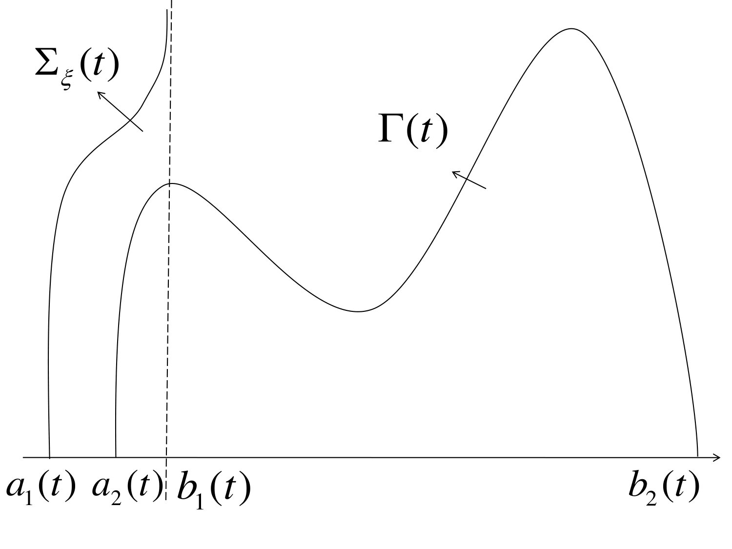 Figure 1
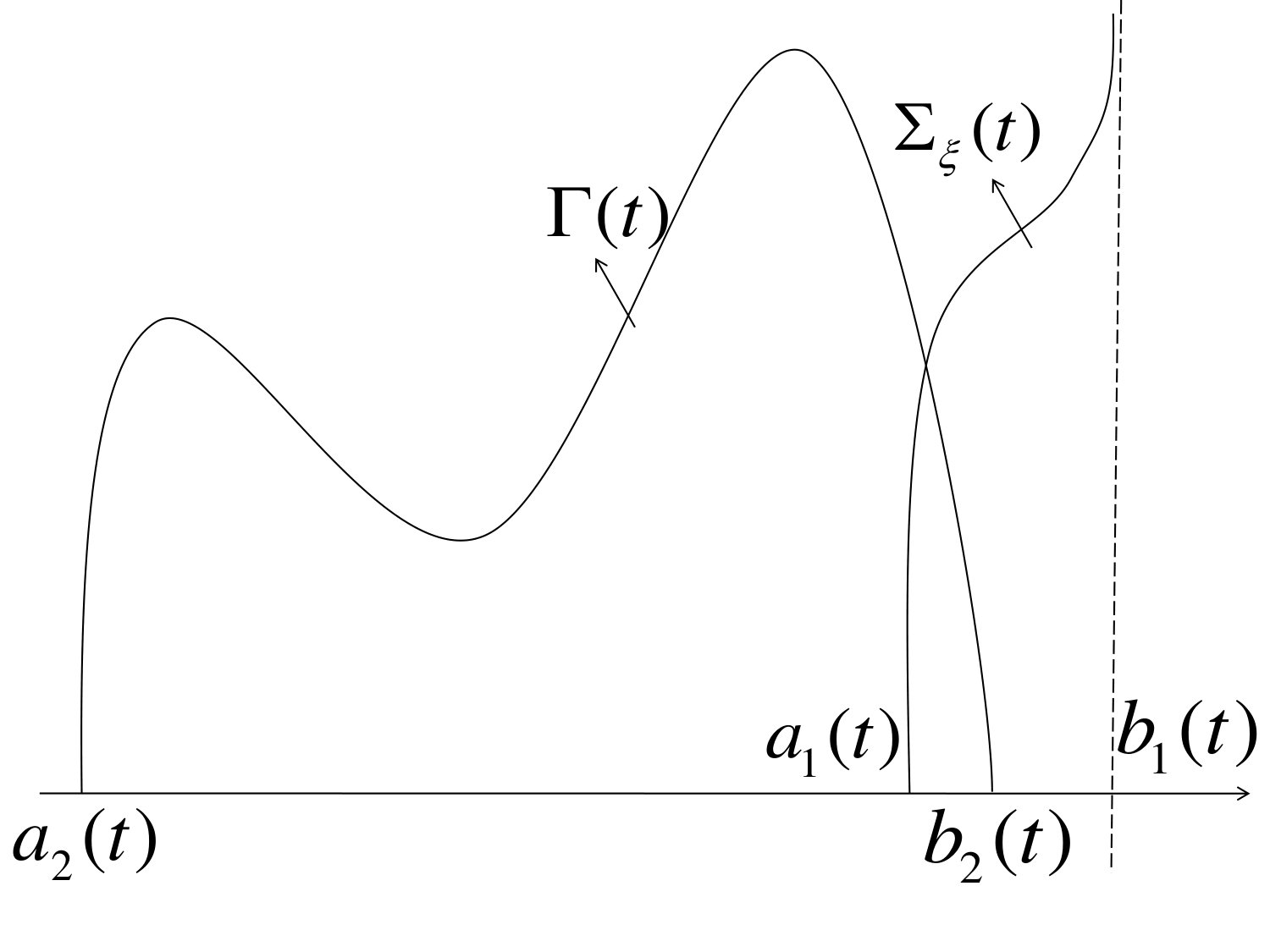 Figure 2
 Figure 3
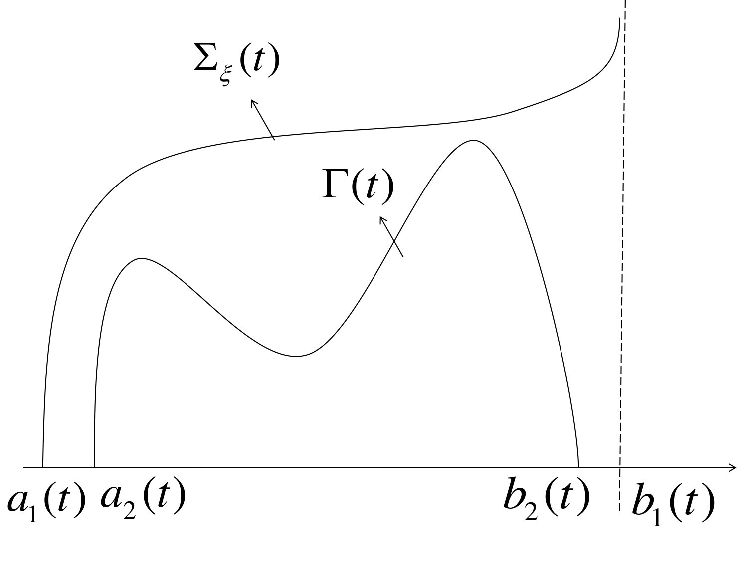 Figure 4
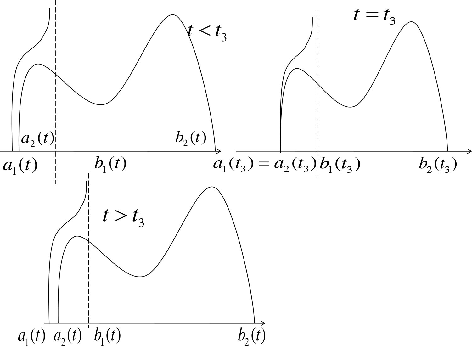 Figure 5
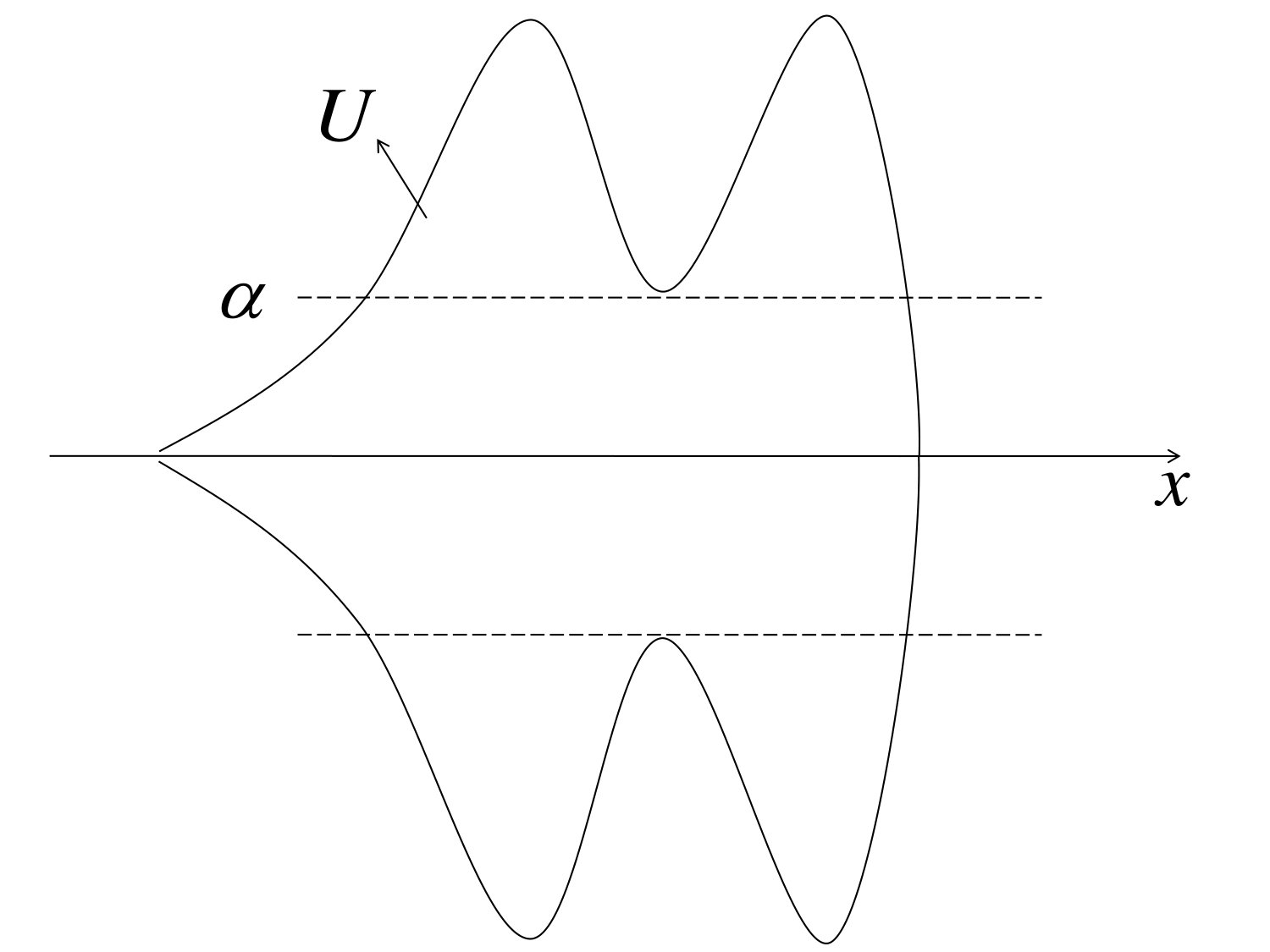 Figure 6
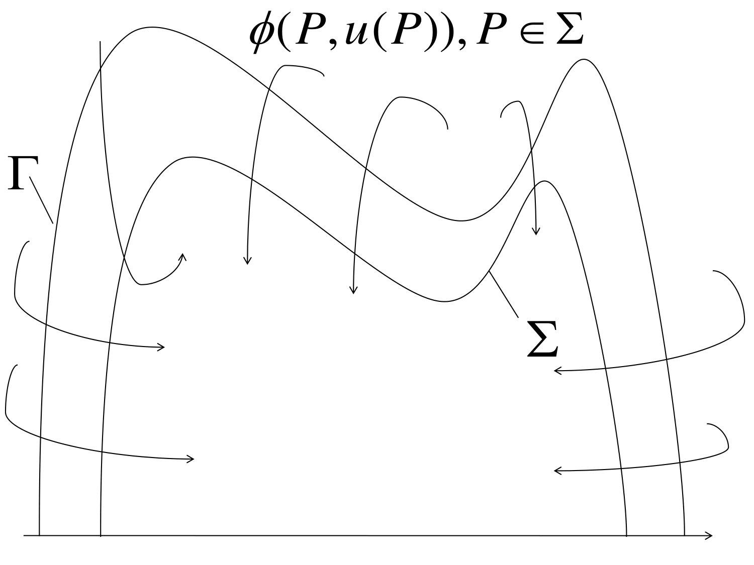 Figure 7
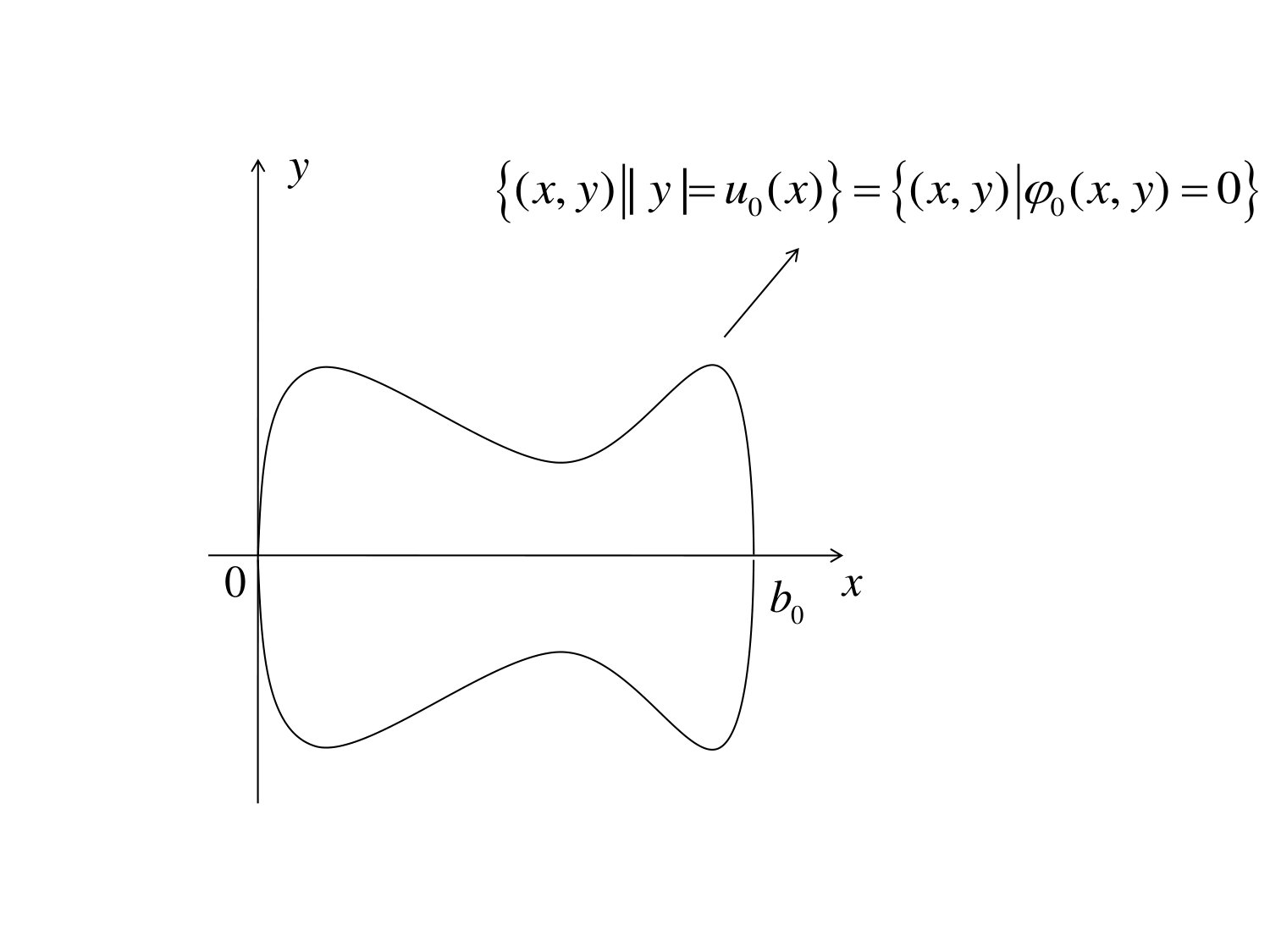 Figure 8
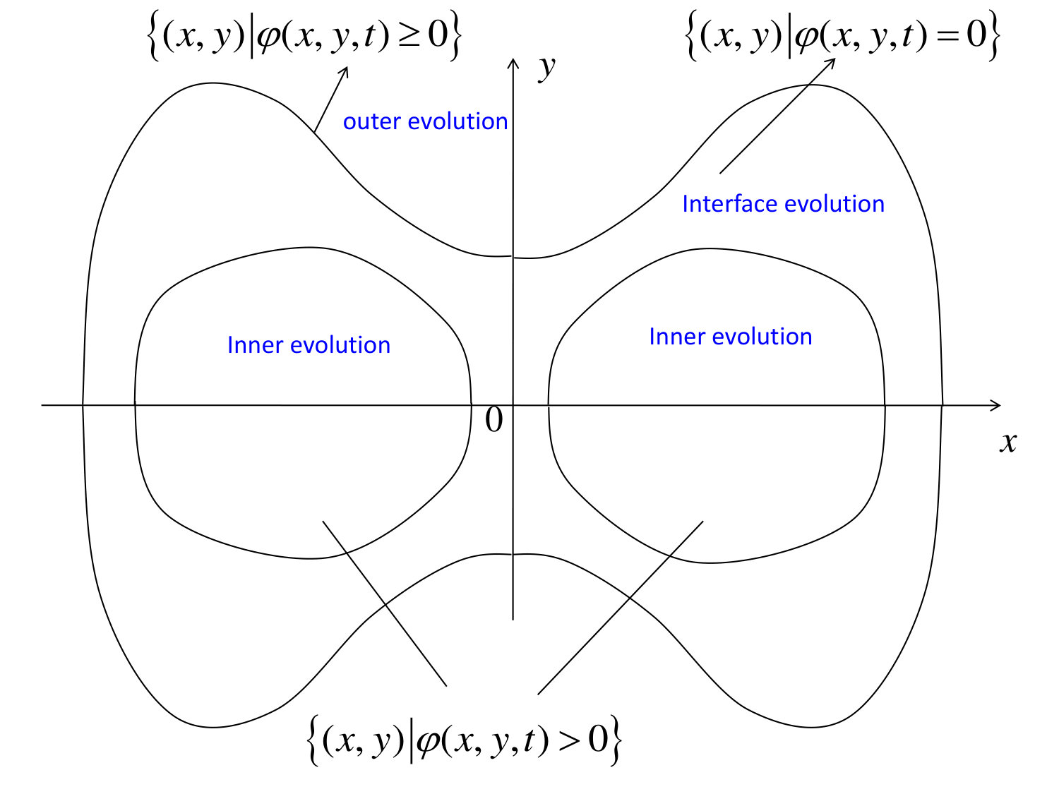 Figure 9
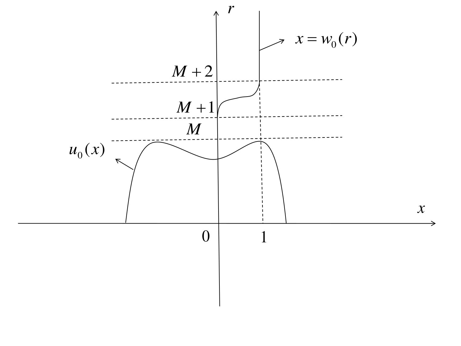 Figure 10
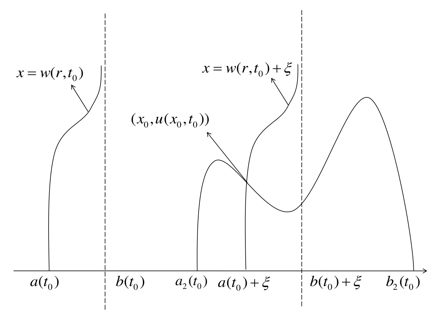 Figure 11
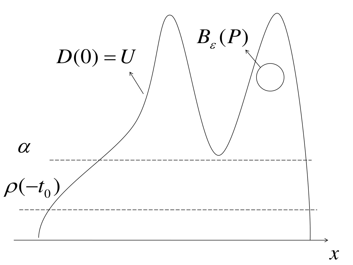 Figure 12
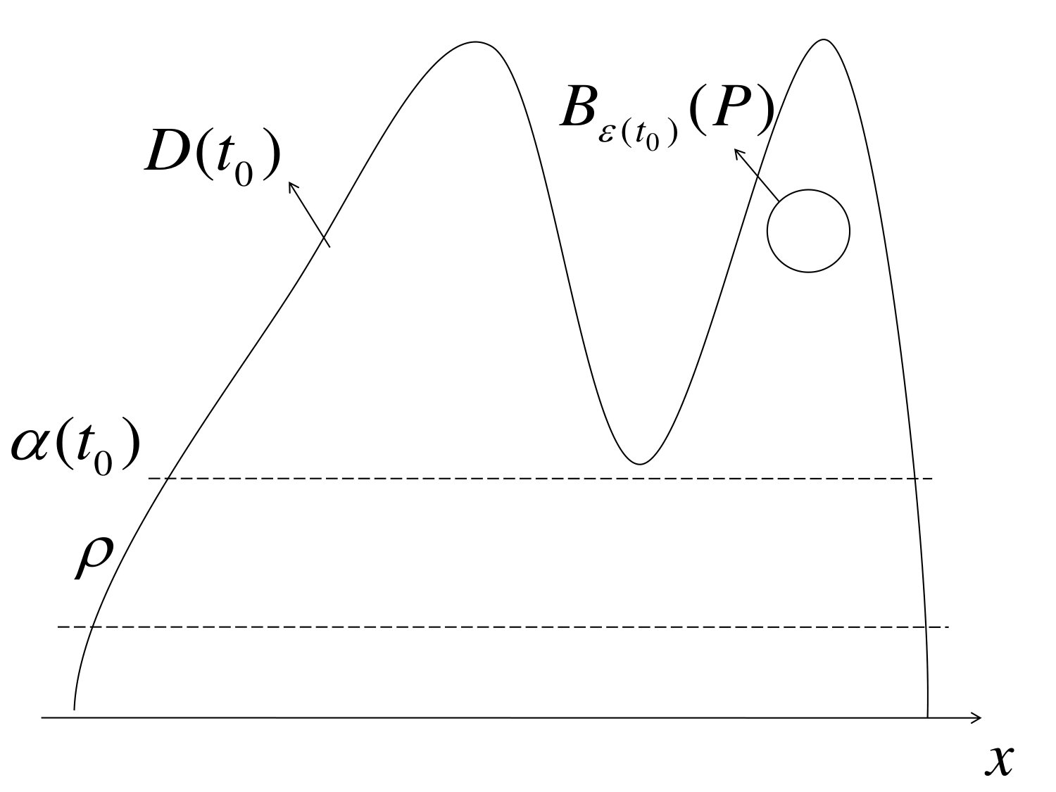 Figure 13
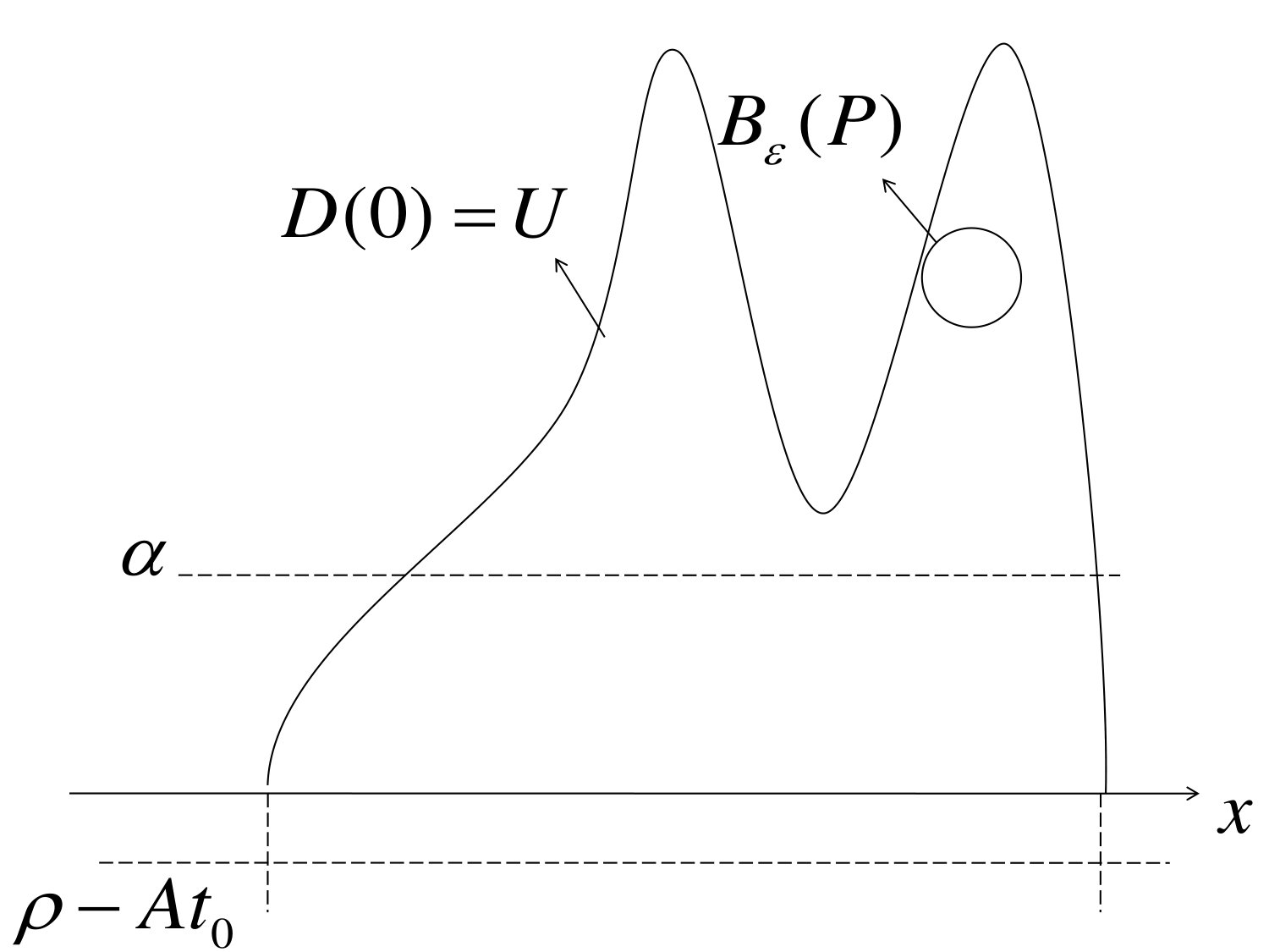 Figure 14
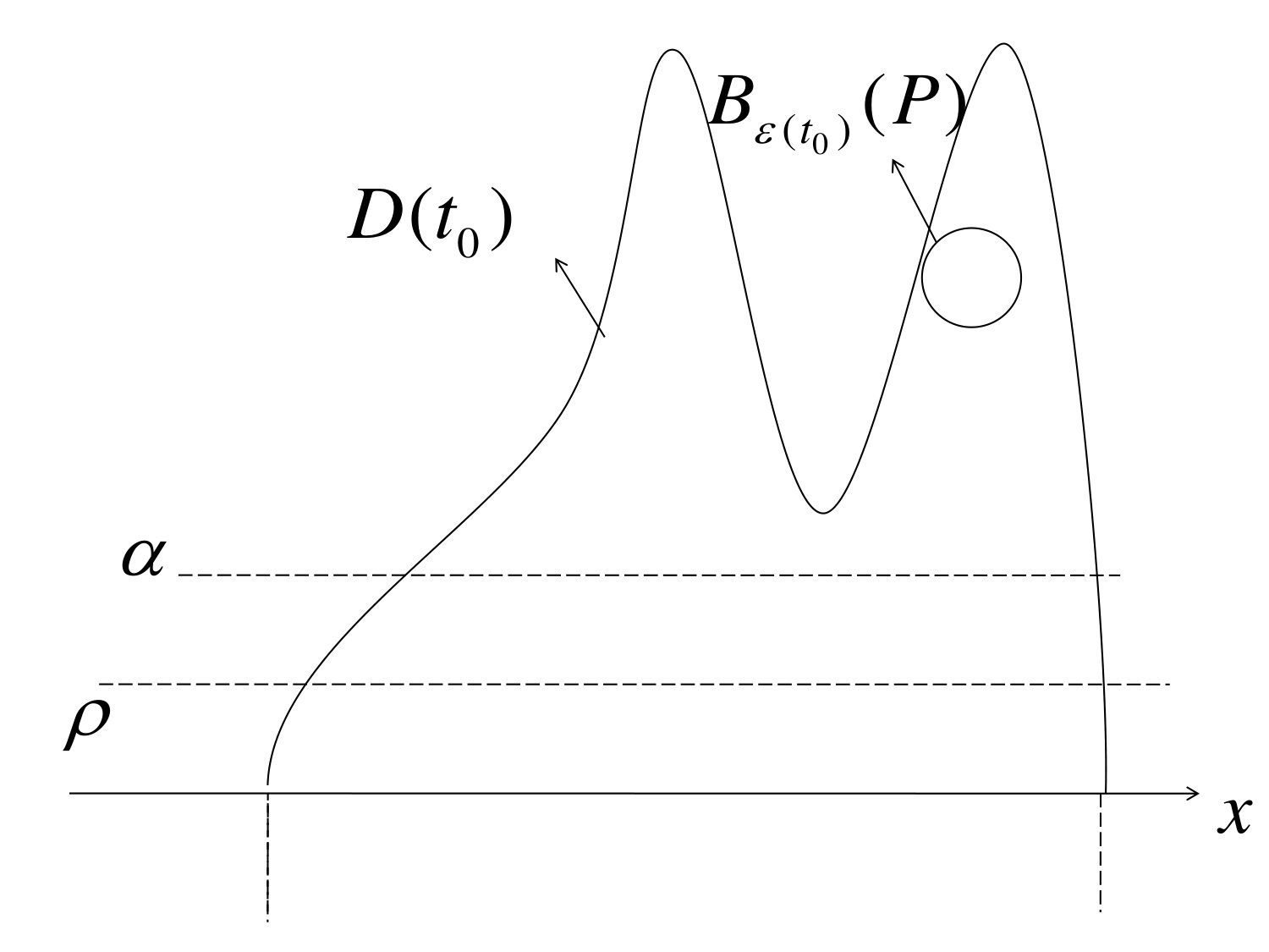 Figure 15
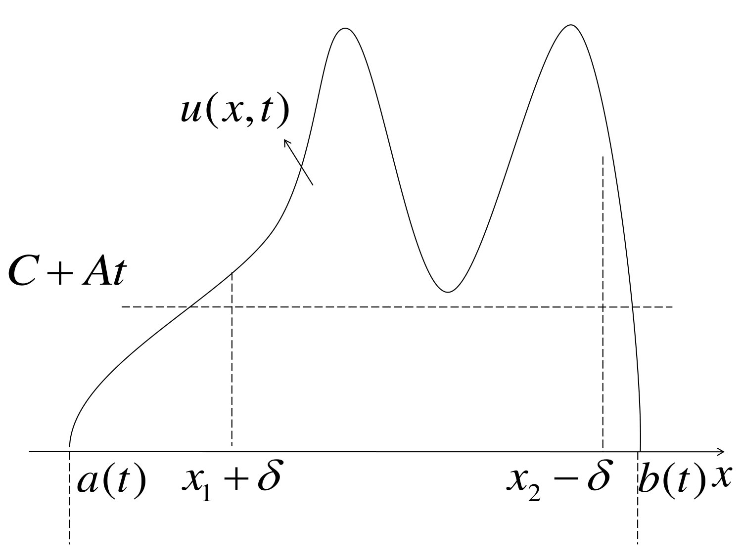 Figure 16
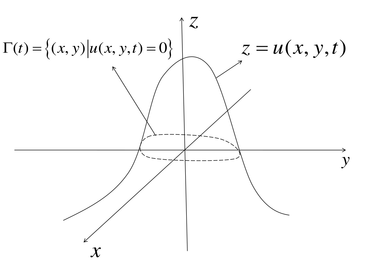 Figure 17
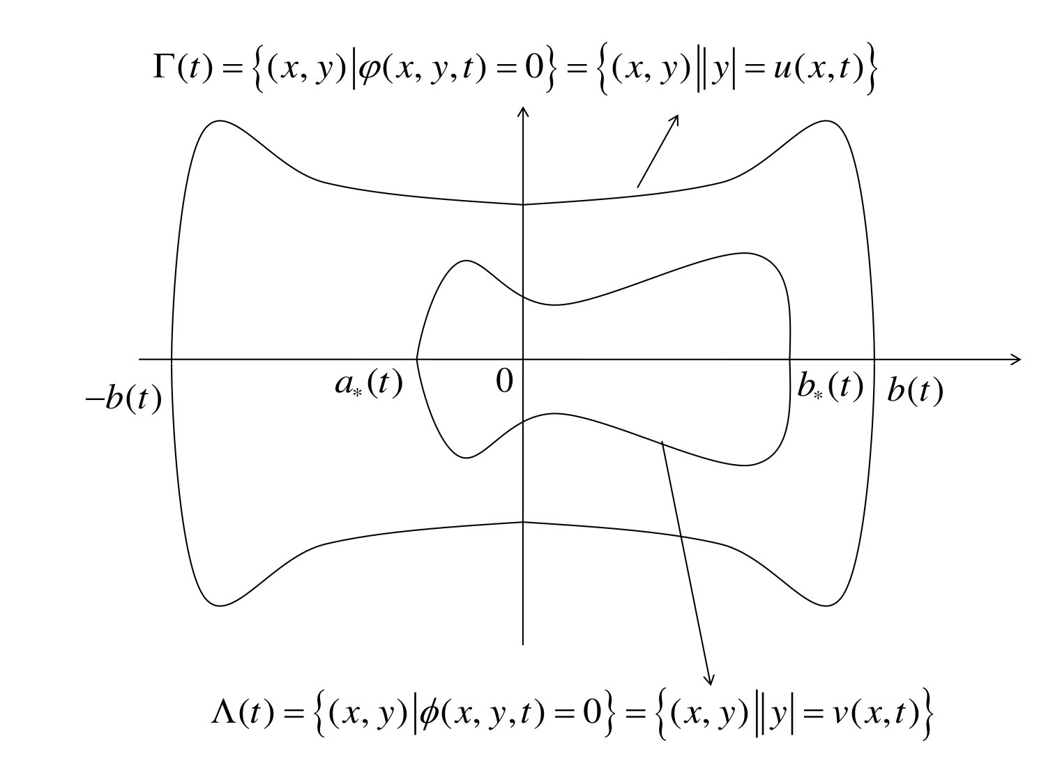 Figure 18
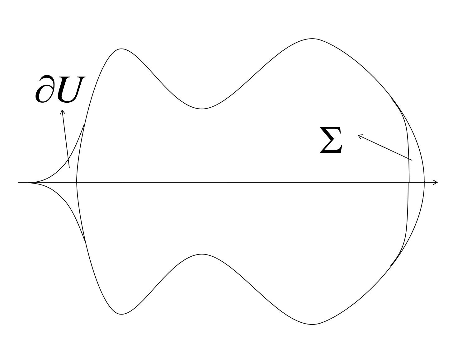 Figure 19
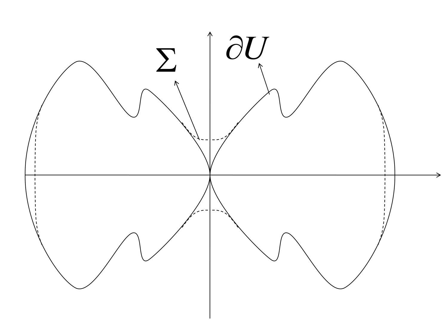 Figure 20
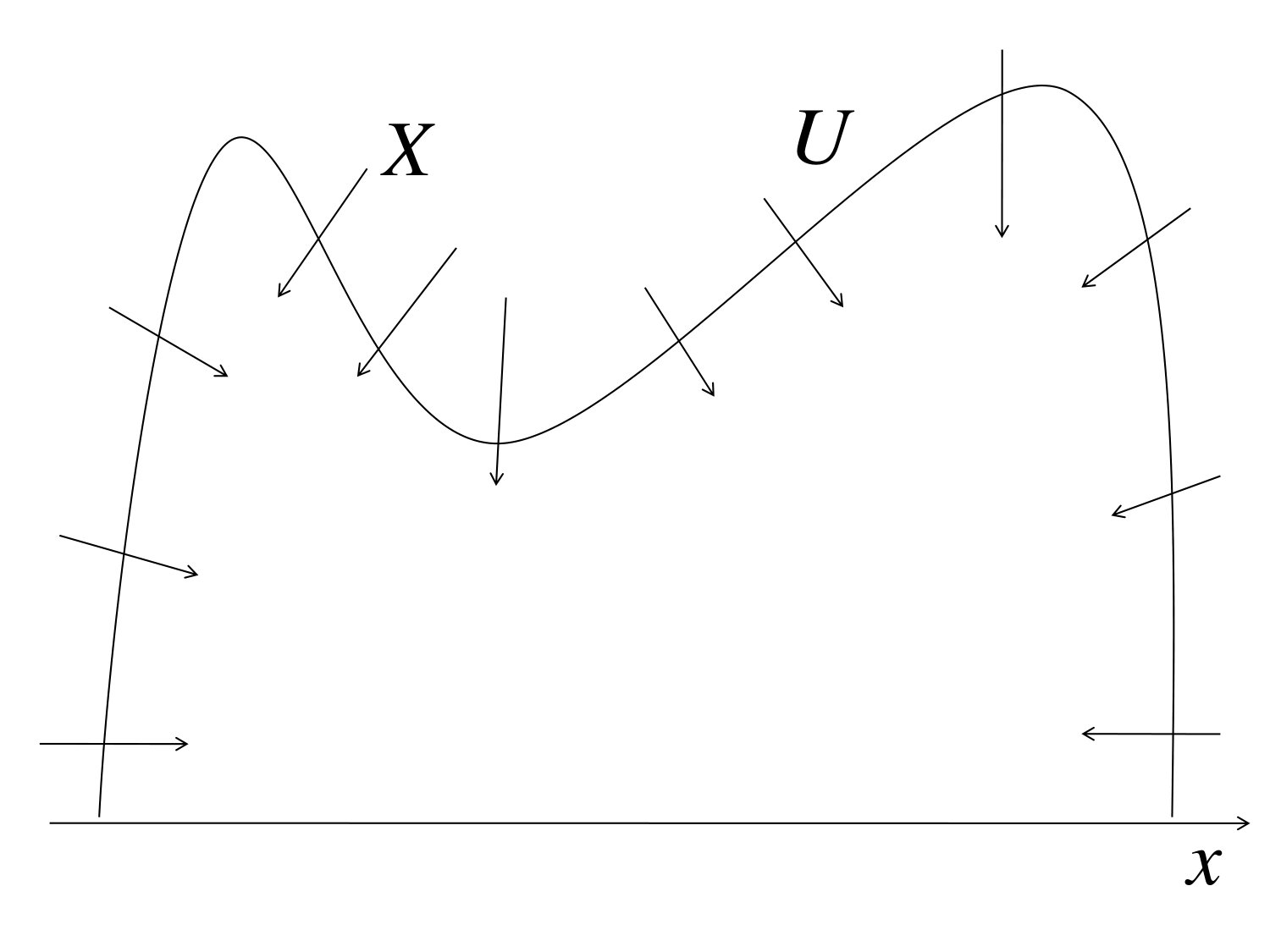 Figure 21
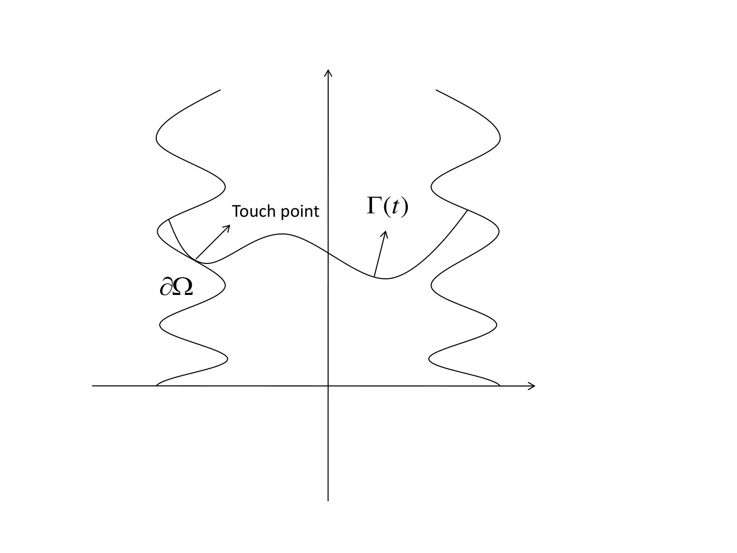 Figure 22
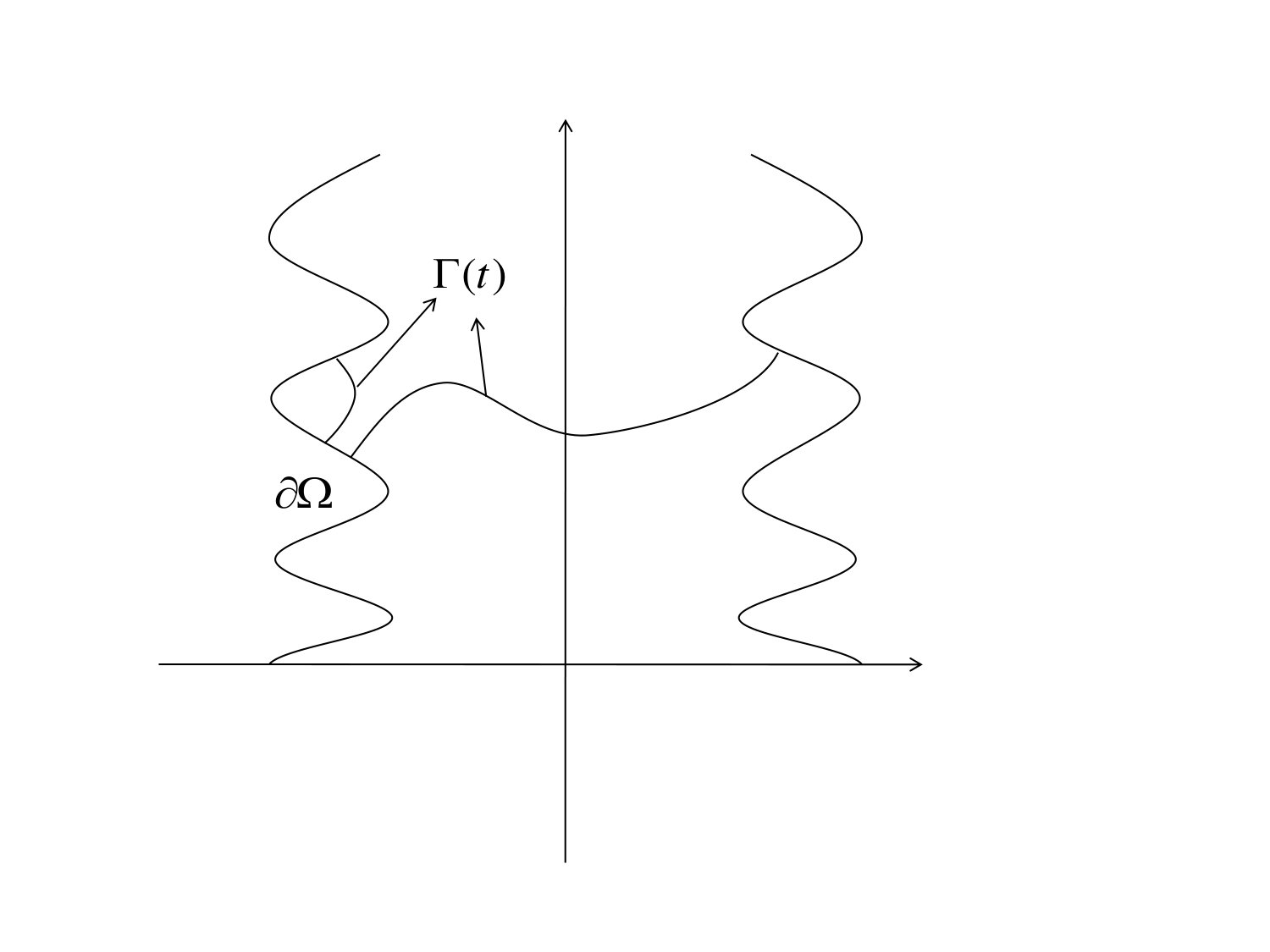 Figure 23
 Figure 24
 Figure 25
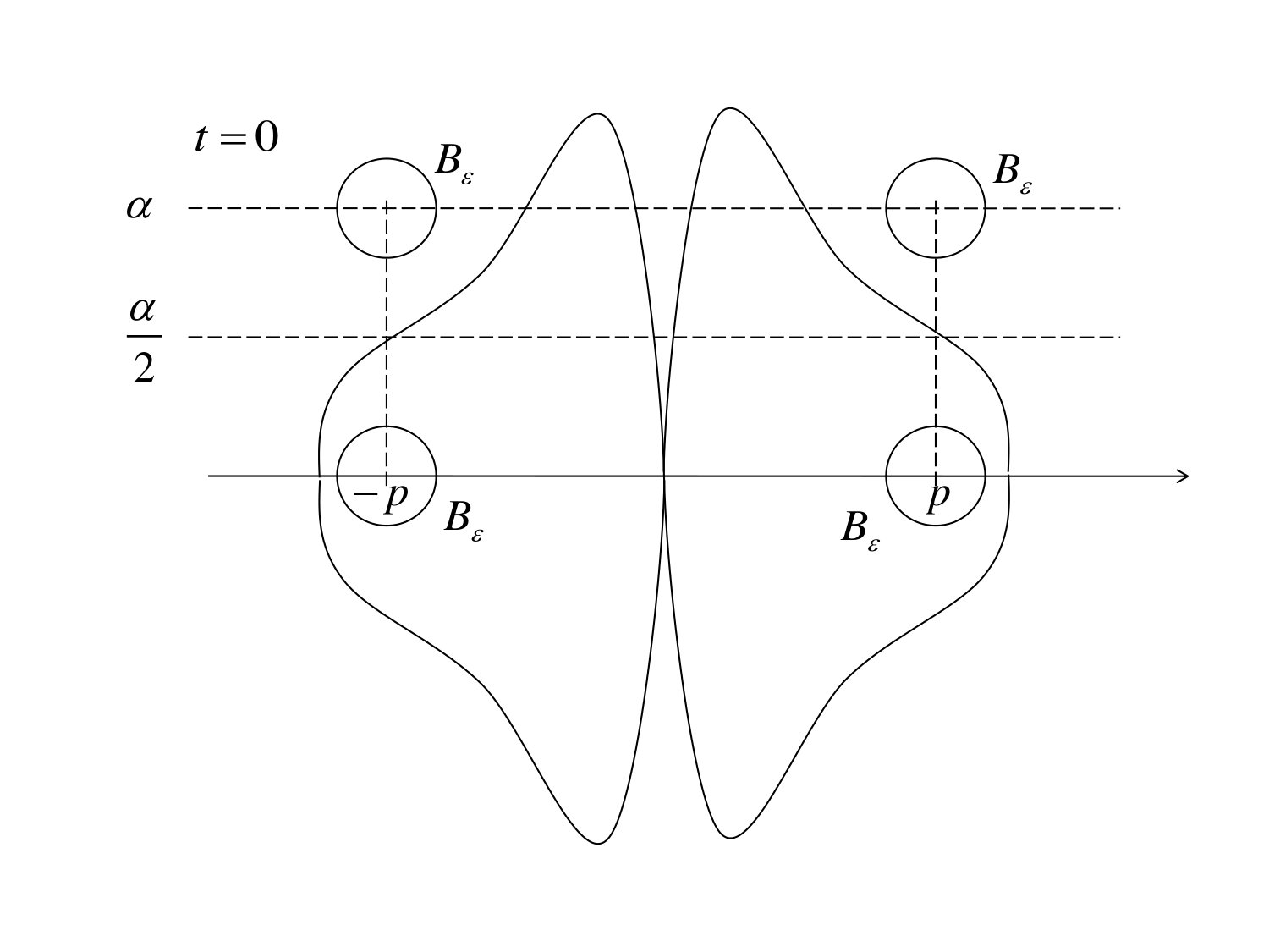 Figure 26
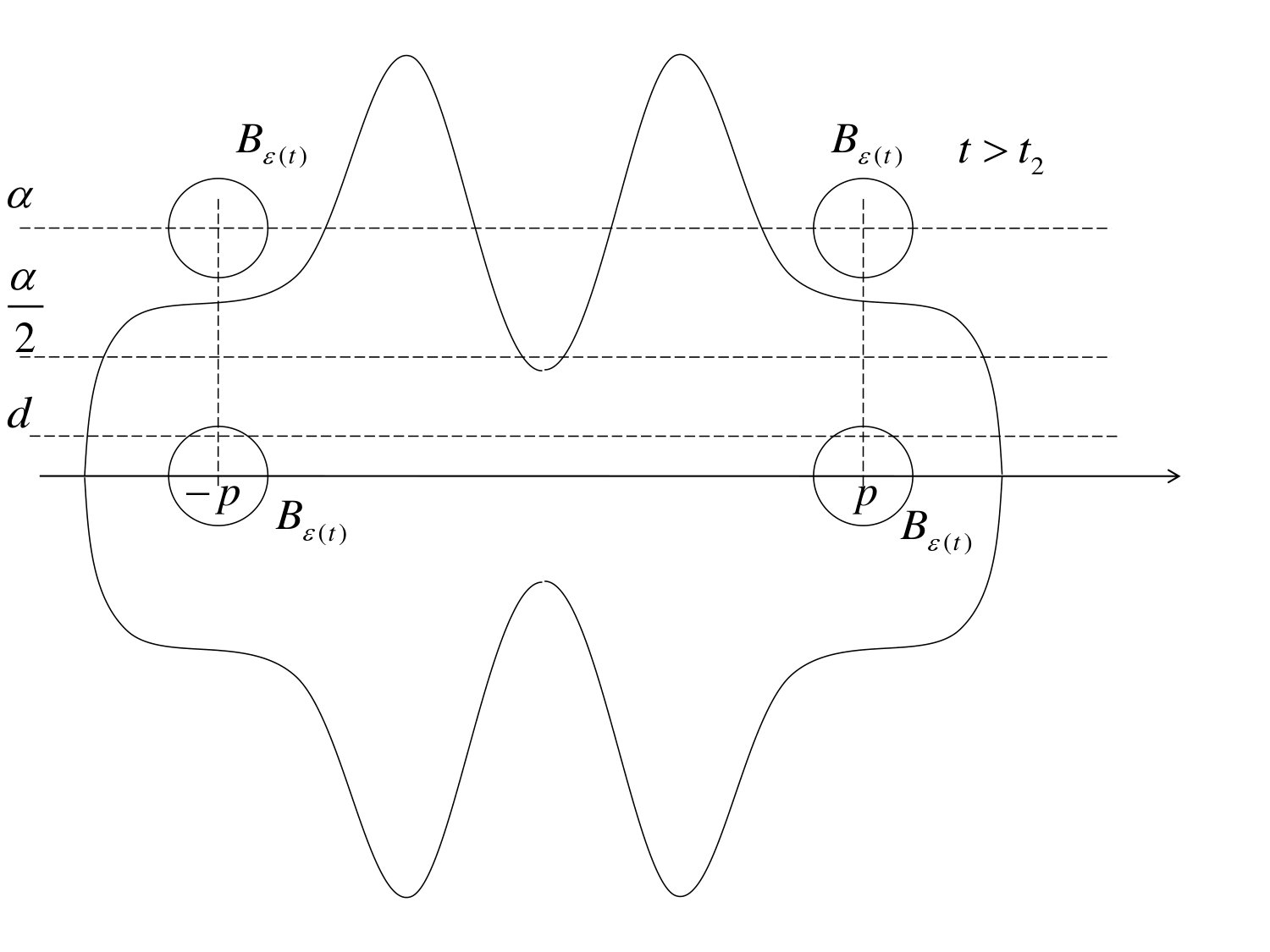 Figure 27