Higher Morse moduli spaces and n-categories
Sonja Hohloch

TL;DR
This paper extends the concept of flow categories in Morse theory to an almost strict n-category framework by iteratively applying Morse theory on Morse moduli spaces, introducing a new categorical structure.
Contribution
It constructs an almost strict n-category from Morse moduli spaces, generalizing previous flow categories to higher categorical levels.
Findings
Established an almost strict n-category structure
Developed suitable Morse functions for higher moduli spaces
Demonstrated the categorical framework's consistency
Abstract
We generalize Cohen & Jones & Segal's flow category whose objects are the critical points of a Morse function and whose morphisms are the Morse moduli spaces between the critical points to an n-category. The n-category construction involves repeatedly doing Morse theory on Morse moduli spaces for which we have to construct a class of suitable Morse functions. It turns out to be an `almost strict' n-category, i.e. it is a strict n-category `up to canonical isomorphisms'.
Click any figure to enlarge with its caption.
 Figure 1
 Figure 2
 Figure 3
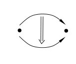 Figure 4
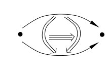 Figure 5
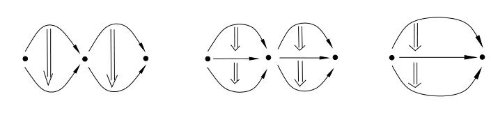 Figure 6
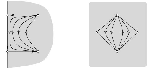 Figure 7
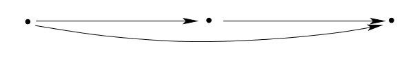 Figure 8
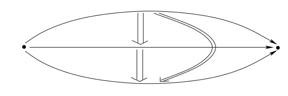 Figure 9
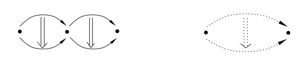 Figure 10
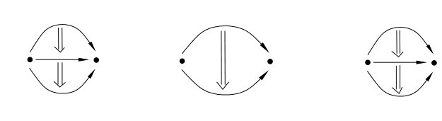 Figure 11
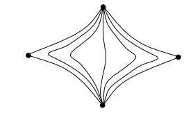 Figure 12
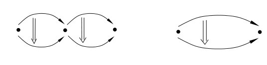 Figure 13
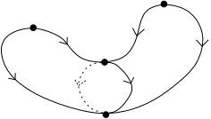 Figure 14
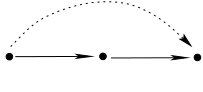 Figure 15
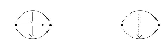 Figure 16
Peer Reviews
No public reviews on file for this paper yet. If you reviewed it on a platform where reviews are public (OpenReview, ICLR, NeurIPS, ICML), you can paste yours below so the community can read it here.
Videos
No videos yet. Explain this paper in a talk, walkthrough, or lecture? Add one.
Taxonomy
TopicsHomotopy and Cohomology in Algebraic Topology · Algebraic structures and combinatorial models · Intracranial Aneurysms: Treatment and Complications
Higher Morse moduli spaces and -categories
Sonja Hohloch
Section de Mathématiques, École Polytechnique Fédérale de Lausanne (EPFL), SB MATHGEOM CAG, Station 8, 1015 Lausanne, Switzerland
Abstract.
We generalize Cohen Jones Segal’s flow category whose objects are the critical points of a Morse function and whose morphisms are the Morse moduli spaces between the critical points to an -category. The -category construction involves repeatedly doing Morse theory on Morse moduli spaces for which we have to construct a class of suitable Morse functions. It turns out to be an ‘almost strict’ -category, i.e. it is a strict -category ‘up to canonical isomorphisms’.
MSC2010 classification: 18B99, 18D99, 37D15, 57R99, 58E05.
Keywords: Morse theory, -category theory, flow category.
The author was partially supported by the DFG grant Ho 4394/1-1.
1. Introduction
The aim of the present paper is to study -category structures in Morse theory. There are (at least) two good reasons to do so: On the one hand, there is an astonishing example and on the other hand there is the natural generalization of a category defined by Cohen Jones Segal [CJS].
Let us first have a look at the seminal example. Let and and consider the -sphere
[TABLE]
with the standard metric. Denote by , the height function of and by and its north and south pole which are the only critical points of . Now consider the compactified Morse moduli space of unparametrized negative gradient flow trajectories between the north and the south pole denoted by . For all , we observe .
This means that we can in fact iterate: Start with and consider with the Morse function . The Morse moduli space is isomorphic to which is a nice manifold. Thus we can consider and choose as Morse function on and obtain the new Morse moduli space . This game can be repeated until . Roughly, we get a ‘filtration’ of Morse moduli spaces with one lying ‘in’ or ‘on’ the other.
A natural question now is: What happens if we start with an arbitrary manifold instead of a sphere? So let be a smooth, closed, -dimensional manifold and a Morse-Smale pair on , i.e. is a Morse function, a Riemannian metric and the (un)stable manifolds intersect each other transversely. The first question is: How do the arising Morse moduli spaces look like? Are they nice enough spaces to admit Morse theory? The literature tells us (cf. Theorem 2) that, under slight assumptions on the metric, the moduli spaces are manifolds with corners, i.e. manifolds modeled on . On manifolds with boundary (possibly with corners), one can do Morse theory as has been shown by Braess [Br], Goresky MacPherson [GM], Akaho [Ak], Kronheimer Mrowka [KM], Ludwig [Lu], Handron [Ha] and Laudenbach [Laud]. On manifolds with boundary, there are two Morse theory approaches possible:
- (1)
Morse functions whose gradient vector field is transverse to the boundary. 2. (2)
Morse functions which induce a gradient vector field tangent to the boundary.
We will use the second option since it is nicely compatible with lower dimensional boundary strata and admits a complete gradient flow. Thus all gradient vector fields in this paper are always tangent to the boundary.
Now let , and consider the moduli space which is a manifold with corners. On we want to choose a Morse function whose gradient vector field is tangent to the boundary. More precisely, instead of ‘boundary’ we should rather speak of boundary strata. The literature tells us (cf. Theorem 2) how the strata look like: The boundary is a union of products of (lower dimensional) Morse moduli spaces. This requires a ‘compatibility condition’ for the Morse function in case different moduli spaces ‘share’ certain strata. Moreover, for reasons which become later apparent, we want the Morse functions to decrease from higher dimensional strata to lower dimensional strata. Such Morse functions can be recursively constructed. Now choose such a Morse function on with a suitable metric, call the Morse function and consider its moduli spaces for , . Once again, if we want to iterate, we have to ask ourselves: What kind of space is ? Can we do Morse theory on it? The construction of , in particular the fact that is decreasing from higher to lower dimensional strata, enables us to prove that is again a manifold with corners (cf. Theorem 5). And this holds true for the Morse moduli spaces of a similar constructed Morse function on such that we can continue to consider Morse moduli spaces on Morse moduli spaces.
We consider the compactified unparametrised moduli spaces such that the dimension decreases at least by one in comparison to the dimension of the space on which we are working. This means that our iteration of Morse moduli spaces on Morse moduli spaces becomes trivial after at most steps.
Before we investigate how the above iteration of moduli spaces gives rise to an -category structure, let us have a look at the second motivation for this paper.
In the 1990’s, Cohen Jones Segal [CJS] came up with the following category: Let be a smooth closed manifold with a Morse-Smale pair . Then the objects of the flow category are given by the critical points of , i.e. , and the morphisms between two objects are given by the compactified Morse trajectory spaces, i.e. for , . According to Cohen Jones Segal [CJS], the classifying space of is homeomorphic to . If the gradient flow is not Morse-Smale the classifying space is only homotopy equivalent to . These are certainly intriguing observations, but we are interested in for a different reason: what is happening if we try to ‘iterate’ this category? With that we mean to introduce a ‘second level’ where the objects are given by the above defined morphisms and the new morphisms are ‘morphisms between morphisms’. More generally, define the objects of the th level to be the morphisms of the th level and the morphisms of the th level to be the morphisms between the morphisms of the th level. This iteration procedure is inspired by a paper by Baez [Ba] where it is used to motivate the notion of -categories.
To the best of our knowledge, it is still not clear what the best definition of an -category is. In the literature, there is a whole zoo of various definitions what -categories are supposed to be. Leinster’s book [Le] gives a good introduction to this topic.
On the first glance, -category theory distinguishes between ‘weak’ and ‘strict’ -categories. This distinction is (among others) related to the question if the composition of morphisms is ‘really’ associative or only associative ‘up to some degree’, i.e. if for the composition of three morphisms , , holds or only where may stand for instance for ‘homotopy equivalent’ or something else.
It is known that ‘weak’ and ‘strict’ -categories are equivalent for , but already for (and higher ) these notions differ. In the following, we will stick to the conventions of Leinster’s book [Le]. The definition of a strict -category is lengthy such that we will not line it out here in the introduction, but we refer the reader to Definition 6 and Definition 7 or directly to Leinster’s book. Since we will not work with weak -categories we also refer the reader to Leinster’s book for their definition.
In this paper, we will show that the iteration procedure of Morse moduli spaces as sketched above will give rise to an almost strict -category. With almost strict we mean that our structure satisfies the conditions of a strict -category up to canonical isomorphisms. Since the ‘up to whatever’-defect of a weak category is usually much bigger than just ‘up to canonical isomorphisms’ we opt for calling the structure ‘almost strict’ instead of ‘not very weak’. This may be up for discussion, but from a geometer’s point of view it makes sense. For a geometer, for example, the cartesian product is associative whereas in fact one probably would have to say ‘associative up to canonical isomorphism’. Since the whole construction of compactified, unparametrized moduli spaces involves already taking equivalence classes etc. we would get nowhere if we would not admit ‘up to canonical isomorphism’ to be negligible. Our contructions certainly do not need ‘too large’ deformations.
Theorem**.**
The above described iteration of Morse moduli spaces can be given the structure of an almost strict -category. The resulting -category is denoted by .
Let us summarize briefly our almost strict -category. The intuitive ‘level structure’ will be replaced by a so-called -globular set (see Definition 6) with source and target functions which ‘remember’ on which ‘level’ an element lives. The elements of our -globular set are tupels of a moduli space and a critical point on this moduli space. The identity functions make use of the stationary moduli spaces . And the composition is based on the gluing of Morse trajectories.
Recall that when we sketched the generalization of the n-sphere example, we required the Morse function to decrease from higher to lower dimensional strata. This is not just a technical assumption. If we admit an arbitrary Morse function, the Morse moduli spaces, more precisely their boundaries, become more complicated. And in particular we do not obtain an -category structure, but rather some ‘opetopes’ (cf. Hohloch Ludwig [HoL]).
So far, each in this way constructed almost strict -category depends on a certain number of chosen Morse data. In order to show independence of the chosen data in Morse or Floer theory, often a so-called ‘homotopy of homotopy’ argument is used (cf. Schwarz [Sch] or Salamon [Sa]). The ‘homotopy of homotopies’ induces a chain homomorphism on the chain complexes associated to the chosen Morse or Floer data. This homomorphism relates the chain complexes similarly as a so-called distributor (cf. Borceux [Bo]) works in category theory. We hope to pursue this idea in a future work in order to relate such Morse -categories to each other, hopefully obtaining an -category of -categories.
Up to the author’s knowledge, the present work is the first one to deal with higher categories associated to Morse theory (with ‘higher’ we mean ). In symplectic geometry and knot theory, -categories appear for example via the Wehrheim-Woodward category (see Wehrheim Woodward [WW] and Weinstein [Wei]) or the -category in Khovanov homology (see Khovanov [Kh]).
To understand the -category of Morse moduli spaces better, the subsequent article Hohloch [Ho] defines two other -categories and and -category functors and . Both categories are motivated by the Morse index and the dimension of the Morse moduli spaces. ‘sees’ the elements of as tuples of vector spaces and homomorphisms spaces between these vector spaces whose dimension is induced by the Morse index and the dimension of the Morse moduli spaces. captures only the Morse indices and thus consists of tuples of (nonnegative) integers. For the exact definitions, we refer the reader to Hohloch [Ho]. Taking and evaluating the Morse index and the dimension of the involved Morse moduli spaces leads to the functors and .
Theorem** (Hohloch [Ho]).**
There are two other almost strict -categories called and and -category functors and .
There were many new algebraic structures discovered and studied in (symplectic) geometry in the last decade which, apart from the already above mentioned reasons, got the author interested in studying new structures in Morse theory. So for instance the graded differential algebra (DGA) appeared, defined for knots and links by Chekanov [Ch], which is a very special case of the more general Symplectic Field Theory (SFT) started by Eliashberg Givental Hofer [EGH].
Organization of the paper
In Section 2, we recall, introduce and construct whatever parts of Morse theory we need in the following sections. In Section 3, we recall the notion of strict -categories. In Section 4, we construct our almost strict -category of Morse moduli spaces. Section 5 calculates some examples.
Acknowledgements
First of all, the author wants to thank Gregor Noetzel for many and lengthy discussions in the beginning of this project. Moreover, the author is indebted to Eric Finster, Kathryn Hess and Michael Warren for explanations of n-category theory and to Dan Burghelea and Ursula Ludwig for discussions and useful hints concerning Morse theory. The author was partially supported by the DFG grant Ho 4394/1-1.
2. Morse moduli spaces
2.1. Notations
Let us start with recalling some notations from Morse theory. There are several approaches to Morse theory: The classical one uses level sets and attaching of handle bodies as e.g. described in Milnor’s book [Mi]. But there is also a dynamical approach via the gradient flow as for instance described in Schwarz’ book [Sch]. We are interested in the dynamical version and summarize the setting briefly.
Let be a closed manifold. A function is called a Morse function if its Hessian is nondegenerate at the critical points . At a critical point , this admits the definition of the Morse index as the number of negative eigenvalues of . Given a Riemannian metric on M, we denote by the gradient of w.r.t. the metric . This leads to the following autonomous ODE of the negative gradient flow of the pair
[TABLE]
Given a critical point , we define the stable manifold
[TABLE]
and the unstable manifold
[TABLE]
A pair is called Morse-Smale if and intersect transversely for all , . We define the Morse moduli space between two critical points and as the space
[TABLE]
consists of the negative gradient flow lines running from to . It can also be identified with . For a Morse-Smale pair , the moduli space is a smooth manifold of dimension . If then the space is empty. Given and , then with is a gradient flow line. Thus the moduli space carries an -action via , . If we divide by the action, we obtain the unparametrized moduli space .
We introduce for , with the notation if .
Before we continue the discussion of the Morse moduli spaces, we need some notation about manifolds with corners. There are different notions and conventions in the literature. Manifolds with corners had been studied first by Cerf [Ce] and Douady [D] at the beginning of the 1960’s. An overview over the various definitions and their differences may be found in Joyce [Jo].
For our purposes, an -dimensional manifold with corners is an -dimensional manifold which is locally modeled on . In order to keep track of the boundary strata, we introduce the following additional notions. Let be an -dimensional manifold with corners and let be a chart. For we define
[TABLE]
is independent of the chosen chart. A face of is the closure of a connected component of . If is the number of faces, we fix an order of the faces and denote them by . The quantity counts the number of faces intersecting in . We call the connected components of the ()-strata of . This yields a filtration and suggests the following definition.
Definition 1**.**
Let be an -dimensional manifold with corners with faces . We call a -manifold if
- (a)
Each lies in faces. 2. (b)
. 3. (c)
For all with the intersection is a face of both and .
In this convention, is again a manifold with corners, but is not. We are following Joyce’s [Jo] definition where the integer has a priori nothing to do with the dimension of the manifold since, in the subsequent work in progress Hohloch Ludwig [HoL], it is convenient to track the intersection behaviour of each face. Note that other authors like Laures [Laur] are defining to be a union of faces which allows choosing .
The standard example of a -manifold is with faces . -manifolds are manifolds without boundary and -manifolds are manifolds with one (smooth) boundary component.
-manifolds have nice properties, see Jänich [Jä], Joyce [Jo], Laures [Laur]. For example, -manifolds can be embedded into an euclidean space such that the faces meet each other perpendicular (cf. so-called neat embeddings in Laures [Laur]). And -manifolds admit well-defined collar neighbourhoods of their boundaries (cf. Laures [Laur]).
Now let us return to Morse moduli spaces. Let for instance be , , with . As sketched in Figure 1 (b), a sequence of trajectories from to may ‘break’ in the limit into trajectories from to and from to . This phenomenon is usually denoted by ‘breaking’ and plays an important role if one wants to compactify unparametrized Morse moduli spaces. More precisely, an unparametrized moduli spaces can be compactified by adding ‘broken trajectories’ and we denote the compactification of via adding broken trajectories by . In order to obtain a nice structure for the compactification one needs to pose conditions on the metric. If is a Morse function and if a metric is euclidean near the critical points of the we call an -euclidean metric.
The following statement was used often as a folklore theorem. Proofs for different settings can be found in Burghelea [Bu], Wehrheim [Weh] and Qin [Qi1], [Qi2]. We summarize the statement as follows.
Theorem 2**.**
Let be a closed manifold, let be Morse-Smale and assume to be -euclidean. Let , with . Then there exists such that is an -dimensional -manifold with corners and its boundary is given by
[TABLE]
where , …, . There is a canonical smooth structure on .
The ‘inverse procedure’ of breaking is ‘gluing’. Roughly, the gluing procedure takes a broken trajectory and yields a Morse trajectory from to . If one wants to glue a multiply broken trajectory the question of associativity of the gluing procedure arises. Gluing is indeed associative and, as a folklore theorem, it has been used a lot in the literature. Recently Qin [Qi3] and Wehrheim [Weh] have written down proofs. For details, we refer to their works.
Theorem 3** ([Qi3], [Weh]).**
Gluing is associative.
2.2. Morse moduli spaces on -manifolds: Our construction
As for manifolds without boundary, there are several ways to define Morse theory on manifolds with boundary. There is the classical approach via handle attachment by Braess [Br] for manifolds with boundary and finally by Goresky MacPherson [GM] for stratified spaces. And there is the newer approach via the gradient flow described by Akaho [Ak] and Kronheimer Mrowka [KM] for manifolds with smooth boundary. Ludwig [Lu] finally defined Morse theory with tangential vector field on stratified spaces.
For our purposes, we are interested in a Morse theory where the gradient vector field is tangential to the boundary. If the gradient vector field is tangent to the boundary it is in particular tangent to all lower strata of the boundary and therefore ‘compatible’ with corners (where it simply vanishes). If we would require the gradient vector field to be transverse to the boundary it would be much more difficult to come up with a consistent definition at the corners.
Working with tangential gradient vector fields is a special case of Ludwig’s [Lu] setting. But since Ludwig [Lu] is interested in setting up a Morse theory, she needs only the one and two dimensional moduli spaces. We are primarily interested in very special constructions of the Morse functions and higher dimensional Morse moduli spaces which are not covered in Ludwig [Lu].
This is the rough outline of the following construction: Consider a Morse function on a smooth manifold. Its compactified Morse moduli spaces are manifolds with corners. On these manifolds with corners we choose ‘good’ Morse functions and consider their compactified Morse moduli spaces which are again manifolds with corners. On these spaces repeat the procedure etc. In each step, we loose at least one dimension since dividing by the -action in reduces the dimension by one. Therefore the compactified moduli spaces will become zero dimensional after a finite number of iterations and the iteration becomes trivial.
Let be a closed manifold. Let be a Morse-Smale pair consisting of a Morse function with -euclidean metric . Let , be distinct critical points and consider . If this moduli space is not empty then, by Theorem 2, it is a manifold (possibly) with corners. The boundary of is of the form
[TABLE]
where , …, . If we apply the formula recursively to the factors of the product we can also write
[TABLE]
Keep in mind that a moduli space may have several connected components. By labelling the components of depth one by , …, , we give the structure of a -manifold for some . In other words, we are dealing with a stratified space. And might share strata with other moduli spaces for , .
Now we want to define a Morse function and a metric on for all , which is compatible with the stratification and the ‘sharing’ of strata. Moreover, the metric should be euclidean near the critical points and the gradient vector field should be tangential to the strata of the boundary. In addition, the flow should flow from higher dimensional strata to lower dimensional strata, but never from lower dimensional strata to higher dimensional ones.
0-strata for :
First recall that is a partially ordered set: We have if and only if there is a flow line from to . Here we also allow the stationary flow line in order to have . If we use the notation we assume . If , the space is zero dimensional (and compact) and thus a finite union of points. Now choose values for on the zero dimensional moduli spaces such that for mutually distinct we have
[TABLE]
where we choose the same value for all connected components of a moduli space. Note that we require the function to be strictly positive. The reason will become apparent later. Moreover assume that different moduli spaces have different values for . Since there are only finitely many critical points we can achieve this easily.
Let us remark that the zero dimensional boundary strata are corners. By construction, they will turn out to be critical points. Note that Akaho [Ak] also constructs his Morse function to be nonzero at the critical points on the boundary.
To the moduli space of stationary curves , we formally assign the value [math] to . (Note that some people consider as the empty set.)
The [math]-strata are automatically critical points since the gradient has to be tangential to all strata meeting at a [math]-dimensional stratum. This is only possible if the gradient vanishes. In accordance with this, we define the metric
[TABLE]
to be euclidean.
Morse functions on cartesian products:
The product structure of the boundary of a compactified Morse moduli space suggests to choose a Morse function on the moduli space which is naturally compatible with the product structure of the boundary. Such Morse functions are obtained as follows: Let and be smooths - resp. -dimensional manifolds equipped with Morse functions and and associated metrics and . On the product , consider , and . It holds
[TABLE]
and therefore if and only if and . We have and thus the set of critical points of with index is given by
[TABLE]
The equation splits into
[TABLE]
and thus there is a flow line from to if and only if there are flow lines and from to and from to . In particular, this requires and . In order to obtain flow lines of relative index 1, either or has to be constant.
Note that one cannot simply identify with . The first space has dimension
[TABLE]
and the second one . Given trajectories and , also and are Morse trajectories. Thus is a solution, but changing changes the geometric shape of and not its parametrisation.
Morse index on strata:
Let be a -manifold with faces , …, . Let and set with . Let be a Morse function. For , we write if for all .
Let , with and a critical point. Then we define the Morse index of as the number of negative eigenvalues of in and abbreviate .
If there are no critical points in a small enough collar neighbourhood of each strata and if the Morse function is constructed radially, one deduces at once:
Remark 4**.**
If the negative gradient flow of a Morse function flows from higher to lower dimensional strata then for all and .
l-strata for with
For higher dimensional strata, we define recursively: Consider , with which implies for in case . Assume that we already defined the Morse function and -euclidean metric in the suitable manner on all [math]-, …, -strata. There are two cases:
Case 1: The boundary is empty: If , then there are no restrictions on the choice of apart from it being larger than on the lower dimensional strata. And the only restriction on is that it has to be euclidean near the critical points of .
Case 2: The boundary is not empty: If
[TABLE]
then the highest dimensional stratum in is an -stratum. In , the highest dimensional one is an -stratum and, on the space , the highest dimensional stratum is an -stratum where . We already have Morse functions and and metrics and on and . For coordinates we define
[TABLE]
on the connected components. Since we required the Morse function to be positive on the zero dimensional moduli spaces, by induction, we have and . The purpose is that the value of rises when we pass from lower to higher dimensional strata since we want the negative gradient flow to flow strictly from higher strata to lower ones.
Analogously we define the metric via
[TABLE]
Note that the product of two euclidean metrics is euclidean. Thus is euclidean near the critical points of .
Now we extend the Morse function and the metric to the interior of such that the gradient vector field is tangential to the boundary, i.e. tangential to every stratum, and the metric is euclidean near the critical points. Moreover, the extension of the Morse function is forbidden to have critical points in an small collar neighbourhood of the boundary (on the boundary, it may have critical points). Explicit examples of this type of construction can be found in Ludwig [Lu] and Akaho [Ak]. One chooses a collar neighbourhood of the boundary and considers its normal bundle. In the interior of a face, one can follow Akaho’s [Ak] construction for manifolds with boundary. He gives an explicit formula for the Morse function. Recall that a corner (or lower boundary stratum) of a -manifold is modeled on a quadrant (or half space) of such that one can construct a suitable Morse function ‘by hand’. Then patch it together. Denote the new Morse function by . Proceed analogously with the metric and make it euclidean near the critical points of the Morse function and obtain .
This finishes the construction of on Morse moduli spaces of : The Morse function takes the cartesian product structure of the boundary into account, behaves naturally with restriction to lower dimensional strata and its negative gradient flow flows strictly from higher strata to lower strata.
The construction of on the moduli spaces of :
Assume for a moment that the negative gradient flow of the Morse function does not only flow from higher to lower, but also from lower to higher strata as sketched below in Figure 1 (a).
As sketched in Figure 1 (a), a trajectory between two critical points and in the interior of the manifold with index difference may actually break via the boundary into three trajectories instead of only two without involvement of the boundary (cf. Figure 1 (b)). This phenomenon is explained in Akaho [Ak] and Kronheimer Mrowka [KM]. It is due to the following observation. W.l.o.g let with and with . Then , i.e. it matters if we consider as critical point of the Morse function as function restricted to the boundary or as function on .
The boundary of the moduli spaces in Figure 1 (a) has still product structure as shown in Akaho [Ak]. But for the -category structure in the later sections we need to be able to ‘compose’ (i.e. glue) two ‘connecting’ trajectories — and we cannot glue just two of the three parts of the broken trajectories in Figure 1 (a) since there is no trajectory from to and also none from to . Therefore we need to exclude such situations if we want to define an -category later on.
This dilemma is solved by using Remark 4: Impose the assumption that the Morse function is increasing from lower dimensional strata to higher dimensional ones. Equivalently, the negative gradient flow flows strictly from higher to lower strata and never from lower to higher strata. Then the Morse index does not depend on the strata and we do not have multiple breaking of trajectries of index difference one. An analogous statement holds true for critical points with higher index difference. We conclude
Theorem 5**.**
Let be a Morse function on a compact -manifold whose negative gradient flow flows from higher to lower strata, but not from lower to higher ones. Assume the metric to be euclidean near the critical points. Let , with . Then there exists such that is an -dimensional -manifold with corners and its boundary is given by
[TABLE]
where , …, . There is a canonical smooth structure on .
Proof.
For and the situation of Figure 1 (a) with this has been proven by Akaho [Ak]. On manifolds with corners and the result is implied by Ludwig [Lu]. The general case goes analogously since Remark 4 reduces the possible breaking phenomena to the case of a closed smooth manifold where Theorem 2 applies. ∎
Altogether, we have so far constructed a Morse function with certain properties on the Morse moduli spaces of . Now we consider the critical points of and the Morse moduli spaces between them. Theorem 5 states that we are again dealing with -manifolds for certain . So we can repeat the construction of a radial Morse function compatible with lower strata now on the Morse moduli spaces of , i.e. there exists a Morse function with similar properties as on the Morse moduli spaces of where , and , .
Once is constructed, its Morse moduli spaces are again -manifolds according to Theorem 5. By construction of the compactified Morse moduli spaces, we always decrease the dimension by (at least) one. Therefore this iteration process terminates after a finite number of repetitions when the moduli spaces become zero dimensional.
Summarizing the above paragraphs, we constructed Morse functions on the compactified Morse module spaces of Morse functions in such a way that each Morse function is compatible with its restriction to lower strata of the Morse moduli spaces of which have the structure of a cartesian product.
3. (Almost) strict -categories
The definition of strict -categories is due to Charles Ehresmann. We recall their definition from Leinster’s book [Le] which gives two equivalent ways of defining strict -categories. One can define it either recursively via enriched categories or direct by listing six properties which have to be satisfied. We focus on the latter definition.
The usual definition of a category will blend into this framework as a -category. Since a category can be considered as a directed graph with structure the way of defining -categories starts as follows.
Definition 6**.**
Given , we define an -globular set to be a collection of sets together with source and target functions , for satisfying and . Elements are called -cells.
To visualize -globular sets, one can think of the -cells as -dimensional disks and sketch them accordingly: a [math]-cell is displayed as a point
[TABLE]
[math]-cells are sometimes also called objects. A -cell with and is sketched as an arrow (or -disk) connecting the [math]-cells and
Sometimes -cells are also called morphisms. A -cell (sometimes called morphism between morphisms) with , and therefore and is sketched as an double arrow or -disk connecting the -cells and
A -cell with and is sketched as a -disk or triple arrow ‘perpendicular to the sheet of paper’
Generally, -cells are represented by an -arrow or a -disk, although sketches clearly reach their limits.
Given -cells , with ‘matching’ source and target conditions , and we are clearly tempted to ‘compose’ and ‘along’ like usual morphisms.
Now consider two -cells , : There are two different ‘matching’ conditions possible: On the one hand, we might have , i.e. we would like to compose and ‘along’ the -cell as sketched in
But, on the other hand, we also can have a matching condition along a [math]-cell as sketched in
which also suggests a composition if we ‘first’ compose the -cells with and with . In fact, as we will see later, it will turn out that there are possible ways to compose -cells, namely along [math]-cells, -cells, …, -cells. Given an -globular set , we express the matching conditions by means of the set
[TABLE]
. More precisely, is the set of -cells which can be composed along a -cell.
Another important feature are identity functions on the -globular set, i.e. a collection of functions for which assign to a -cell a certain -cell with source and target . For [math]-cells, this means
And for -cells, this leads to
In the following definition, we will pose additional conditions on the composite and identities.
Definition 7**.**
Let . A strict -category is an -globular set equipped with
- •
a function for all . We set and call it composite of and .
- •
a function for all . We set and call it the identity on .
These have to satisfy the following axioms:
- (a)
(Sources and targets of composites)* For and we require*
[TABLE] 2. (b)
(Sources and targets of identities)* For and we require*
[TABLE] 3. (c)
(Associativity)* For and , , with , we require*
[TABLE] 4. (d)
(Identities)* For and we require*
[TABLE] 5. (e)
(Binary interchange)* For and , , , with*
[TABLE]
we require
[TABLE] 6. (f)
(Nullary interchange)* For and we require .*
If and are strict -categories we define a strict -functor as a map of the underlying -globular sets commuting with composition and identities. This defines a category Str--Cat of strict -categories.
Slightly relaxing the requirements, we define
Definition 8**.**
An almost strict -category satisfies the requirements of a strict -category up to canonical isomorphism.
The compatibility of the identities with the source and target functions in item (d) of Definition 7 can be visualized via
The binary interchange of item (e) in Definition 7 can be sketched as
And the nullary interchange looks like
4. The -category of Morse trajectory spaces
4.1. -globular set of Morse moduli spaces
In the following, we will define the -globular set of Morse moduli spaces on which the -category of Morse moduli spaces is based.
Let be a compact -dimensional -manifold with a Morse function (constructed as in the previous section) and a -euclidean metric . We set
[TABLE]
Given two critical points , , we consider the space . On this space, we choose a Morse function with -euclidean metric as described in Subsection 2.2. We define
[TABLE]
The index of the Morse function or metric starts with the number of the level on which the function or metric lives and continues with the (history of) critical points which gave rise to the moduli space. The upper row states the source points and the lower row the target points. It is important to keep carefully track of the ‘history’ of a moduli space. Analogously, given , , choose a Morse function and -euclidean metric on and let
[TABLE]
We work with tupels (point, moduli space) instead of only the moduli spaces in order to obtain well-defined source and target function. We iterate this process and obtain for
[TABLE]
Since dividing by the action in the construction of the compactified moduli spaces reduces the dimension by one, we can iterate this procedure at most times before the moduli spaces in question become zero dimensional and the iteration in turn becomes trivial.
For , we define source and target functions
[TABLE]
via
[TABLE]
and set for
[TABLE]
Lemma 9**.**
* is an -globular set.*
Proof.
A short calculation yields and . ∎
Now we define the -cells which can be composed along -cells:
[TABLE]
How do this elements look like? For and , an element given by
[TABLE]
satisfies . More generally, an element given by
[TABLE]
is characterized by
[TABLE]
Therefore we introduce the following more natural notation for tuples . For , we set and . For the index , we set , and . For , we keep the , , and . For , this new notation leads to
[TABLE]
where one can easily see the meaning of being in : Both -cells arise, up to level , from the same critical points . At level , we have the matching condition There are no additional conditions on the critical points on the higher levels apart from the ones required in the definition of . We call the history of up to level . In this new notation, it holds for the critical points
[TABLE]
If in the two expressions above then there are no ’s and ’s resp. ’s and ’s in the index of the function.
4.2. The identities
In order to turn the -globular set into an almost strict -category, we need to define the composite and the identities.
Let us start with the identities. They are supposed to be functions for . For , the set consists of the critical points . Let and identify with the moduli space . Then identify with the only critical point on . Thus we have . With this in mind, we set
[TABLE]
For , we set for
[TABLE]
where we again identified . For , this gives us functions
[TABLE]
which will be our candidates for the identity functions of an -category generated by Morse moduli spaces.
4.3. Motivation for the composite of Morse moduli spaces
Now we address the composite of the future -category. Since this paper also addresses readers from geometry and topology to whom the index consuming and somewhat confusing notation of -categories may be unfamiliar, we will introduce the composite step by step for small and . Experienced or hurried readers may skip ahead a few pages — the general formula is given in the next subsection.
Consider the case and . We have
[TABLE]
and define the composite via
[TABLE]
In terms of -category language, we composed the two 1-cells , along the 0-cell :
Geometrically, this describes the gluing procedure of Morse trajectories as lined out for instance in Schwarz [Sch] and sketched below.
is contained in the boundary of . Thus the point lies in (the boundary of) . It is a critical point of the Morse function .
Now consider the case and and the space given by
[TABLE]
and define
[TABLE]
Geometrically, we are doing the same as for except that we are on the space instead of : we glue the Morse trajectories from to (i.e. ) with the Morse trajectories from to (i.e. ). In terms of -category language, we glue the 2-cells and along the 1-cell as visualized below.
4.4. General case: The composite of Morse moduli spaces
After spending some time on motivating the composite for small , we now define the composite for arbitrary . To simplify notation, we treat the three cases and and separately.
Case and
There are no ’s and ’s such that the ‘history index’ starts with , , . We set
[TABLE]
Case and
We set
[TABLE]
Case and
There are no ’s, ’s, ’s and ’s in the ‘history index’ which ends with , , . We set
[TABLE]
4.5. The -category of Morse moduli spaces
After defining an -globular set, identity functions and a composite we formulate the main theorem of this paper.
Theorem 11**.**
The -globular set together with the above defined identity functions and composites is an almost strict -category .
Proof.
(a) Source and targets of composites: Let . Show that, for , we have and .
For , we compute
[TABLE]
For , we find
[TABLE]
Similar computations yield .
Furthermore, we have to prove the following. For , show that, for , we have and .
For , we compute
[TABLE]
The case follows similarly. And an analogous computation yields the claim for the target function.
(b) Sources and targets of identities: We need to show that . Letting , we compute
[TABLE]
and similar for the target function.
(c) Associativity of the composite: Given and , , we need to prove .
We set
[TABLE]
and compute
[TABLE]
where
[TABLE]
On the other hand, we obtain
[TABLE]
where
[TABLE]
Geometers usually consider the cartesian product as associative, but if one wants to be rigorous, it is certainly associative up to canonical isomorphism. And the same holds for the gluing of Morse trajectories (cf. Theorem 3). Thus, possibly up to canonical isomorphism, . Note that for and , the associativity of the composite reduces to the associativity of the gluing procedure:
[TABLE]
(d) Identities: For and , we have to show
[TABLE]
Let and compute
[TABLE]
where we identified the critical point with the moduli space and with the critical point on the moduli space etc. Thus we obtained times in each line of the subscript. Now we compute
[TABLE]
Since the product of a space with a point can be canonically identified with the space itself we conclude (up to canonical isomorphism)
[TABLE]
which yields the claim. The proof for the source function requires the identification of
[TABLE]
with
(e) Binary interchange: Given and , and , , we need to show .
The requirements on , , and lead to
[TABLE]
We compute
[TABLE]
where
[TABLE]
and is given by
[TABLE]
On the other hand, we calculate
[TABLE]
where
[TABLE]
and is given by
[TABLE]
and share the first half
[TABLE]
and differ in the second half only up to exchange of the second and third coordinate in the 4-tuples. Thus, up to canonical isomorphism, we obtain the claim.
(f) Nullary interchange: For and , we need to show .
Let
[TABLE]
and compute
[TABLE]
which finishes the proof of Theorem 11. ∎
5. Examples
5.1. The standard -sphere
Consider the -dimensional sphere with the height function , as Morse function and use the induced metric from . It has two critical points and , namely the north and the south pole, with and . Thus we have
[TABLE]
The moduli space can be identified with which has no boundary. Thus there are no lower dimensional boundary strata which could impose compatibility conditions on the chosen Morse function on the Morse moduli space. Let be the height function on with critical points (north pole) and (south pole). We obtain
[TABLE]
The moduli space can be identified with and we choose as Morse function the height function on . We get
[TABLE]
where is the north pole and the south pole. Iterating this procedure, we find eventually
[TABLE]
where can be identified with which again can be identified with the critical points . The process terminates with
[TABLE]
where the ‘point’ can be identified with the ‘space’ and similar for .
Now we want to look for the possible composites. For sake of readability, we only consider the case . The general case goes analogously. Moreover, to simplify notation, we drop the Morse function in the moduli spaces. We compute
[TABLE]
and conclude
[TABLE]
And computing
[TABLE]
yields
[TABLE]
Calculating
[TABLE]
leads to
[TABLE]
Geometrically the lack of composites is due to the fact that there are only two critical points on each level such that there is no gluing or breaking of Morse trajectories.
5.2. The deformed -sphere
Let be the deformed 2-sphere
Choose the induced metric from (suitably adjusted near the critical points) and take the height function, denoted by , as a Morse function. The Morse trajectories are the negative gradient flow lines. For sake of readability, we drop the Morse function in the notion of the moduli spaces. We have four critical points with Morse index , , and . For the moduli spaces holds and with cardinality , and . All other moduli spaces vanish. has two connected components which we denote by .
We have . is an interval whose boundary is given by
[TABLE]
and similar for . If we consider the (components of one of the) zero dimensional moduli spaces as points instead of spaces, we write instead of . Now define the Morse function as follows. Assume on and on to be strictly monotone with the same (positive) maximum at and the same (positive) minimum at which are the only critical points. With this notion, we find
[TABLE]
We compute
[TABLE]
We compute the composite
[TABLE]
The other elements of work similarly. Geometrically we are gluing Morse trajectories. Now abbreviate
[TABLE]
and we obtain
[TABLE]
The appearing moduli spaces are singletons such that for will only contain ‘trivial’ elements of the form . We compute
[TABLE]
which implies
[TABLE]
and we compute for instance
[TABLE]
which is due to the fact that we are working on a space which consists of a single point. Moreover we have
[TABLE]
and we compute
[TABLE]
The reference list from the paper itself. Each links out to its DOI / PubMed record.
- 1[Ak] Akaho, M.: Morse Homologies and manifolds with boundary , Comm. in Contemp. Math. 9 , no. 3 (2007), 301 – 334.
- 2[Ba] Baez, J.: An introduction to n-categories , in Category theory and Computer Science (Santa Margharita Ligure 1997) , Lecture Notes in Computer Science 1290, Springer 1997.
- 3[Bo] Borceux, F.: Handbook of categorical algebra 1: Basic category theory , Cambridge University Press 1994.
- 4[Br] Braess, D.: Morse-Theorie für berandete Mannigfaltigkeiten , Math. Ann. 208 , 133 – 148 (1974).
- 5[Bu] Burghelea, D.: Smooth structure on the moduli space of instantons of a generic vector field. Geometry-Exploratory Workshop on Differential Geometry and its Applications, 37 – 59, Cluj Univ. Press, Cluj-Napoca, 2011.
- 6[Ce] Cerf, J.: Topologie de certains espaces de plongements , Bull. Soc. math. France 89 (1961), 227 – 380.
- 7[Ch] Chekanov, Y.: Differential algebra of Legendrian links , Invent. Math. 150 (2002), no. 3, 441 – 483.
- 8[CJS] Cohen, R.; Jones, J.; Segal, G.: Morse theory and classifying spaces , Preprint.