Exponential convergence of solutions for random Hamilton-Jacobi equations
Renato Iturriaga, Konstantin Khanin, Ke Zhang

TL;DR
This paper proves that solutions to certain randomly kicked Hamilton-Jacobi equations on the torus converge exponentially fast to a stationary solution, advancing understanding in stochastic PDEs.
Contribution
It establishes exponential convergence for solutions of multi-dimensional random Hamilton-Jacobi equations, completing a significant research program.
Findings
Solutions converge exponentially fast to stationary solutions almost surely.
The results extend previous work to multi-dimensional settings.
Completes the theoretical framework for stochastic Hamilton-Jacobi equations.
Abstract
We show that for a family of randomly kicked Hamiton-Jacobi equations on the torus, almost surely, the solution of an initial value problem converges exponentially fast to the unique stationary solution. Combined with the results in \cite{IK03} and \cite{KZ12}, this completes the program started in \cite{EKMS00} for the multi-dimensional setting.
Click any figure to enlarge with its caption.
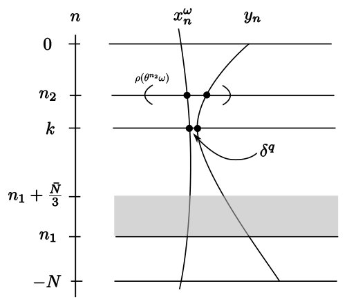 Figure 1
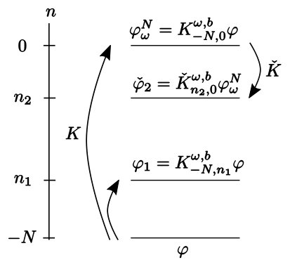 Figure 2
Peer Reviews
No public reviews on file for this paper yet. If you reviewed it on a platform where reviews are public (OpenReview, ICLR, NeurIPS, ICML), you can paste yours below so the community can read it here.
Videos
No videos yet. Explain this paper in a talk, walkthrough, or lecture? Add one.
Taxonomy
TopicsGeometry and complex manifolds · Quantum chaos and dynamical systems · Geometric Analysis and Curvature Flows
Exponential convergence of solutions for random Hamilton-Jacobi equations
Renato Iturriaga
CIMAT, Guanajuato, Mexico
,
Konstantin Khanin
University of Toronto
and
Ke Zhang
University of Toronto
Abstract.
We show that for a family of randomly kicked Hamiton-Jacobi equations on the torus, almost surely, the solution of an initial value problem converges exponentially fast to the unique stationary solution. Combined with the results in [6] and [8], this completes the program started in [4] for the multi-dimensional setting.
1. Introduction
We consider the randomly forced Hamilton-Jacobi equation on the dimensional torus
[TABLE]
where , stands for gradient in , and is a random potential. By writing , we obtain the stochastic Burgers equation
[TABLE]
with the condition . This is one of the motivations of our study. On the other hand, (1.1) is a particular example of the more general Hamilton-Jacobi equation
[TABLE]
where is strictly convex and superlinear in (called the Tonelli Hamiltonians). Many of our results can be generalized to (1.3), but we will restrict to (1.1) for simplicity.
We are interested in two types of random potentials. In [4], the authors consider the dimension , with the “white noise potential”
[TABLE]
where are smooth functions, and are independent white noises. It is shown that finite time solutions of (1.1) converges exponentially fast to a unique stationary solution. In this paper, we generalize this result to arbitrary dimensions, for a related “kicked” model.
The “kicked force” model was introduced in [6], with
[TABLE]
where is an i.i.d. sequence of potentials, and is the delta function. We focus on the “kicked” potential (1.5) as it is simpler, but retains most of the features of the system.
The system (1.3) does not admit classical solutions in general, and the solution is interpreted using the Lax-Oleinik variational principle. There is a semi-group family of operators (see (2.2))
[TABLE]
such that the function , is the solution to (1.1) on the interval with the initial condition .
It is shown in [6] that under suitable conditions on the kicked force, almost surely, the system (1.1) admits a unique solution (up to an additive constant) on the interval . Let us denote
[TABLE]
which is the suitable semi-norm for measuring convergence up to an additive constant. Then any solution on converges to as , uniformly over all initial conditions in the semi-norm :
[TABLE]
Our main result is that the above convergence is exponentially fast.
Main result**.**
There exists a (non-random) such that, almost surely,
[TABLE]
see Theorem 1.
Remark*.*
Exponential convergence is also known to hold in the viscous equation
[TABLE]
(see [11]). However, in this case the a priori convergence rate as . Since our result provides a non-zero lower bound on convergence rate when , it is an interesting question whether a uniform rate of convergence exists for the viscous equation.
The a priori convergence rate of the Lax-Oleinik semi-group is only polynomial in time, as evidence in the case when there is no force, i.e. . In the case when the force is non-random, exponential convergence is true when the Aubry set consists of finitely many hyperbolic periodic orbits or fixed points ([7]). According to a famous conjecture of Mañe, this condition holds for a generic force ([9]), however this conjecture is only proven when among forces ([2], [3]).
In some sense, [8] proves a random version of Mañe’s conjecture. In the random case, the role of the Aubry set is taken by the the globally minimizing orbit, and it is shown that this orbit is non-uniformly hyperbolic under the random Euler-Lagrange flow. Conceptually, this hyperbolicity then allows the exponential convergence. However, this is quite delicate. To illustrate, let us outline the proof in the uniform hyperbolic case:
- •
(Step 1) Consider a solution that is sufficiently close to the stationary solution , this is the case since we know the solution , albeit without any rate estimates.
- •
(Step 2) Show that the associated finite time minimizers is close to the Aubry set when . By hyperbolic theory, any orbit that stays in a neighborhood of an hyperbolic orbit for time must be exponentially close to it at some point.
- •
(Step 3) Finite time minimizer being exponentially close to the Aubry set implies the solution is in fact exponentially close to .
In the non-uniform hyperbolic case, Step 2 fails, because a non-uniform hyperbolic orbit only influence nearby orbits in a random neighborhood whose size changes from iterate to iterate. We are forced to devise a much more involved procedure:
- (1)
(Step A) Reduce the problem to a local one, where we only study the solution in a small (random) neighborhood of the global minimizer. 2. (2)
(Step B) Consider a solution is -close to the stationary solution locally. Use a combination of variational and non-uniform hyperbolic theory to show that the finite time minimizer is -close to the global minimizer at some time, where . This step can only be done up to an exponentially small error. 3. (3)
(Step C) Use step B to show the solution is -close to the stationary solution. Feed the new estimates into Step B, and repeatedly upgrade until is exponentially small.
We now present the outline of the paper. We formulate our assumptions and main result in Section 2. Basic properties of the viscosity solutions and stationary solutions are introduced in Sections 3 and 4. In Section 5, we reduce the main result to its local version, as outlined in Step A. This is Proposition 5.1.
In Section 6, we describe the upgrade procedure outlined in Step C. Step B is formulated in Proposition 6.1, and the proof is postponed to Sections 7 and 8.
2. Statement of the main result
Consider the kicked potentials (1.5), where the random potentials are chosen independently from a distribution , with .
Given an absolutely continuous curve , we define the action of to be
[TABLE]
In other words, when are integers, we include the kick at time , but not at time . For , and , the action function is
[TABLE]
where is absolutely continuous. The action function is Lipshitz in both variables.
The backward Lax-Oleinik operator is defined as
[TABLE]
We take (2.2) as the definition of our solution on with initial conditon . Due to the fact that vanishes at non-integer times, is completely determined by its value at integer times. In the sequel we consider only . The operators satisfies a semi-group property: for ,
[TABLE]
We now state the conditions on the random potentials. The following assumptions are introduced in [6], which guarantees the uniqueness of the stationary solution.
- Assumption 1. For any , there exists s.t. has a maximum at and that there exists such that
[TABLE]
- Assumption 2. .
- Assumption 3. There exists such that has a unique maximum.
The following is proved in [6] under the weaker assumption that :
Proposition 2.1**.**
[6]**
- (1)
Assume that assumption 1 or 2 holds. For a.e. , we have the following statements.
- (a)
There exists a Lipshitz function , , such that for any ,
[TABLE] 2. (b)
For any , we have
[TABLE] 2. (2)
Assume that assumption 3 holds. Then the conclusions for the first case hold for .
We now restrict to a specific family of kicked potentials. The following assumption is introduced in [6].
- Assumption 4. Assume that
[TABLE]
where are smooth non-random functions, and the vectors is an i.i.d sequence of vectors in with an absolutely continuous distribution.
In [8], a stronger assumption is used to obtain information on the stationary solutions and the global minimizer. These additional structures provides the mechanism for exponential convergence. Let be the density of .
-
Assumption 5. Suppose assumption 4 holds, and in addition:
-
–
[TABLE]
- –
For every , there exists non-negative functions and such that
[TABLE]
where , .
Assumption 5 is rather mild. We only need to avoid the case that is degenerate in some directions. In particular, it is satisfied if are i.i.d. random variables with bounded densities and finite mean.
We now state the main theorem of this paper.
Theorem 1**.**
- (1)
Assume that assumption 5 and one of assumption 1 or 2 hold. Assume in addition that the mapping
[TABLE]
is an embedding. For , let be the unique stationary solution in Proposition 2.1. Then there exists a (non-random) and a random variables such that almost surely, for all ,
[TABLE] 2. (2)
Assume that assumption 3 and 5 hold. Then the same conclusions hold for .
3. Viscosity solutions and the global minimizer
Let be an interval. An absolutely continuous curve is called a minimizer if for each interval , we have . In particular, is called a forward minimizer if , a backward minimizer if and a global minimizer if .
Due to the kicked nature of the potential, a minimizer is always linear between integer times. Then any minimizer is completely determined by the sequence
[TABLE]
The underlying dynamics for the minimizers is given by family of maps
[TABLE]
The maps belong to the so-called standard family, and are examples of symplectic, exact and monotonically twist diffeomorphisms. For , , denote
[TABLE]
The (full) orbit of a vector is given by the sequence
[TABLE]
If is a minimizer, then defined in (3.1) is an orbit, namely
[TABLE]
In this case, we extend the sequence to and call a minimizer.
The viscosity solution and the minimizers are linked by the following lemma:
Lemma 3.1** ([8], Lemma 3.2).**
- (1)
For and , for each there exists a minimizer such that , and
[TABLE]
Moreover, the minimizer is unique if is differentiable at , and in this case . 2. (2)
Suppose is the stationary solution. Then at every and , there exists a backward minimizer such that
[TABLE]
Moreover, the minimizer is unique if is differentiable at , and in this case .
In case (1) we call a minimizer for , and in case (2) the orbit is called a minimizer for .
The forward minimizer is linked to the forward operator , defined as
[TABLE]
Analog of Proposition 2.1 and Lemma 3.1 hold, which we summarize below.
- •
For every , almost surely, there exists a unique Lipshitz function , , such that
[TABLE]
- •
For each there exists a minimizer such that and
[TABLE]
When is differentiable at we have .
- •
For each , and , there exists a forward minimizer such that ,
[TABLE]
and if is differentiable at .
The global minimizer is characterized by both and .
Proposition 3.2**.**
Assume that Assumption 4 holds, and one of Assumptions 1 and 2 holds. Assume in addition, the map (2.4) is an embedding. Then for , almost every , there exists a unique global minimizer . For each , is the unique reaching the minimum in
[TABLE]
Moreover, are both differentiable at , and .
The function
[TABLE]
will serve an important purpose for the discussions below.
The random potentials are generated by a stationary random process, so there exists a measure preserving transformation on the probability space satisfying
[TABLE]
The family of maps then defines a non-random transformation
[TABLE]
on the space . Then from Proposition 3.2,
[TABLE]
and the probability measure
[TABLE]
is invariant and ergodic under . The map , where is the group of all symplectic matrices, defines a cocycle over . Under Assumption 5, its Lyapunov exponents are well defined, and due to symplecticity, we have
[TABLE]
and .
There is a close relation between the non-degeneracy of the variational problem (3.4), and non-vanishing of the Lyapunov exponents for the associated cocycle.
Proposition 3.3** ([8], Proposition 3.10).**
Assume that assumption 5 and one of assumptions 1 or 2 holds. Assume in addition that the map (2.4) is an embedding. Then for all , for a.e. , the following hold.
- (1)
There exist depending only on in (2.4) and the density of , and a positive random variable such that
[TABLE]
with
[TABLE] 2. (2)
The Lyapunov exponents of satisfy
[TABLE]
The second conclusion of Proposition 3.3 implies the orbit for the sequence of maps is non-uniformly hyperbolic. In particular, it follows that there exists local unstable and stable manifolds. It is shown in [8] that the graph of the gradient of the viscosity solutions locally coincide with the unstable and stable manifolds.
Proposition 3.4** ([8], Theorem 6.1).**
Under the same assumptions as Proposition 3.3, for each , there exists positive random variables , , such that the following hold almost surely.
- (1)
There exists embedded submanifolds and , such that
[TABLE]
for all . 2. (2)
For every , let and be the backward and forward minimizers satisfying . Then
[TABLE]
[TABLE]
where .
Remark*.*
In Lemma 4.9 we will show that the random variables in item (2) can be chosen to satisfy an additional tempered property.
4. Properties of the viscosity solutions
4.1. Semi-concavity
Given , we say that a function is semi-concave if for any , there exists a linear form such that
[TABLE]
A function is called semi-concave if it is semi-concave as a function lifted to . The linear form is called a subdifferential at . If is differentiable at , then the subdifferential is unique and is equal to . A semi-concave function is Lipshitz.
Lemma 4.1** ([5], Proposition 4.7.3).**
If is continuous and semi-concave on , then is -Lipshitz.
Lemma 4.2** ([5]).**
Suppose both and is semi-concave, then over the set , are differentiable, , and is -Lipshitz over the set .
Let and . The action function has the following properties.
Lemma 4.3** ([8], Lemma 3.2).**
- (1)
*The function is **semi-concave in the second component, and is *semi-concave in the first component. Here is the time-shift, see (3.6). 2. (2)
For any , and , the function is semi-concave, and is semi-concave. Either function, as well as the sum of the two functions, are Lipshitz. 3. (3)
For , the functions is semi-concave, and is semi-concave, Either function, as well as the sum of the two functions, are Lipshitz.
We first state two lemmas concerning the properties of the Lax-Oleinik semigroup, the goal is to obtain Lemma 4.7, which is a version of Mather’s graph theorem ([10]).
Lemma 4.4**.**
For any , , , we have
[TABLE]
Proof.
For any ,
[TABLE]
then
[TABLE]
∎
Lemma 4.5**.**
Suppose . Let be a minimizer for in the sense of (3.3). Then for each , we have
[TABLE]
and
[TABLE]
Proof.
By definition , so the case is trivial. For , we have
[TABLE]
Then
[TABLE]
On the other hand, apply Lemma 4.4 to and yields
[TABLE]
The lemma follows. ∎
As a result, A minimizer of a backward solution is also a minimizer of the forward-backward solution.
Corollary 4.6**.**
Let be a minimizer for , then it is also a minimizer for .
Proof.
Using the calculations in the proof of Lemma 4.5, we get
[TABLE]
for all . The corollary follows. ∎
The following lemma provides a Lipshitz estimate for the velocity of the minimizer in the interior of the time interval.
Lemma 4.7**.**
Suppose with . Let and be two minimizers for in the sense of (3.3). Then for all , we have
[TABLE]
The same conclusion hold, if and are minimizers for .
Proof.
We apply Lemma 4.5 to and . Denote and , since , is semi-concave, is semi-concave. Since , Lemma 4.2 and Lemma 3.1 implies
[TABLE]
∎
4.2. Properties of the stationary solutions
Recall that
[TABLE]
which takes its minimum at the global minimizer . To simplify notations, we will drop the subscript from these functions when there is no confusion.
This function is very useful, as it can be used to measure the distance to the global minimizer. For all , we have
[TABLE]
Moreover, is a Lyapunov function for infinite backward minimizers. Namely, if is a backward minimizer, then for any , we have
[TABLE]
(See [8], Lemma 7.2)
Let us also recall, for any , there exists functions , such that for all backward minimizers such that
[TABLE]
We will also use a process in non-uniform hyperbolicity known as tempering.
Lemma 4.8** ([1], Lemma 3.5.7).**
Let be a random variable satisfying , then for any , there exists such that
[TABLE]
Let’s call a random variable tempered if for any , both admits an upper bound satisfying (4.4). Products and inverses of tempered random variables are still tempered.
The random variables in (4.1) and in (4.3) are tempered.
Lemma 4.9**.**
For any , there exists random variables
[TABLE]
such that
[TABLE]
Proof.
Lemma 4.8 applies to and since . The fact that and are tempered can be proven by adapting the proof Theorem 6.1 in [8]. We now explain the adaptations required.
In [8], there exists local linear coordinates with the formula centered at the global minimizer , with the estimates (section 6 of [8]). Then it is shown that there exists a random variable (called in that paper) such that any orbit must be contained in the stable manifold. is tempered because it is the product of tempered random variables. Indeed, the following explicit formula was given in the Proof of Theorem 6.1, section 7 of [8]:
[TABLE]
where are the same as in this paper, and the fact that are tempered is explained in Lemma 6.5 and Proposition 7.1 of [8]. We now convert to the variable . Since the norm of the coordinate changes are tempered, there exists a tempered random variable such that any orbit contained in
[TABLE]
must be contained in the unstable manifold of .
We now show the same conclusion holds on a neighborhood of the configuration space , with tempered. Let and let be its backward image. According to Lemma 4.2, , as a result
[TABLE]
Finally, using (4.1) and (4.2), we have
[TABLE]
We obtain that
[TABLE]
implies is contained in the unstable manifold of . is tempered as it is products of tempered random variables.
The fact that an orbit on the stable manifold of a non-uniformly hyperbolic orbit converge at the rate , and that the coefficient is tempered is a standard result in non-uniform hyperbolicity, see for example [1]. ∎
We now use what we obtained to get an approximation for the stationary solutions.
Lemma 4.10**.**
There exists , , such that for all , and , we have
[TABLE]
We also have the forward version: for ,
[TABLE]
Proof.
We only prove the backward version. By definition,
[TABLE]
On the other hand, let be the minimizer for , then
[TABLE]
where is from Lemma 4.9. The lemma follows by repeating the calculation with , and taking . ∎
5. Reducing to local convergence
In this section we reduce the main theorem to its local version.
Proposition 5.1**.**
Under the same assumptions as Proposition 3.3, there exists , positive random variables , , and such that for all and ,
[TABLE]
The proof of Proposition 5.1 is given in the next section. Next, we have a localization result, which says any minimizer for or go through the neighborhood at time , when are large enough.
Proposition 5.2**.**
Under the same assumptions as Proposition 3.3, let be a positive random variable. Then there exists depending on such that the following hold.
- (1)
For any , let , be a (backward) minimizer for . Then . 2. (2)
(The forward version) For any , let , be a (forward) minimizer for . Then .
We prove Proposition 5.2 using the following lemma, stating that the Lax-Oleinik operators are weak contractions.
Lemma 5.3** ([6], Lemma 3).**
For any , we have
[TABLE]
Proof of Proposition 5.2.
We only prove item (1), as the (2) can be proven in the same way. We denote, for ,
[TABLE]
and let , be a minimizer for . For each , Lemma 4.4 and 4.5 implies
[TABLE]
[TABLE]
hence
[TABLE]
Recall that for , we have is the unique minimum for . Define
[TABLE]
By Proposition 2.1, we can choose large enough such that for ,
[TABLE]
As a result, there exists a constant such that
[TABLE]
It follows that the minimum in (5.1) is never reached outside of . We obtain . ∎
We now prove our main theorem assuming Proposition 5.1.
Proof of Theorem 1.
It suffices to prove the theorem for .
Let us apply Proposition 5.2 with from Proposition 5.1. Let be a minimzier of , and a minimizer for
[TABLE]
with , and . According to Proposition 5.1, there exists such that for all ,
[TABLE]
Then
[TABLE]
On the other hand,
[TABLE]
Using , combine both estimates, and take supremum over all , we get
[TABLE]
In order to shift the end time to , let denote for . Fix some such that , then by ergodicity, almost surely, for infinitely many . Let us define as the largest such that , then
[TABLE]
provided . By reducing and taking larger we can absorb the constant . ∎
6. Local convergence: localization and upgrade
In this section we prove Proposition 5.1 (local convergence) using Proposition 6.1 and a consecutive upgrade scheme. It is useful to have the following definition for book keeping.
Definition**.**
Given , , let be a minimizer for , we say the orbit satisfies the (backward) approximation property if for every such that , we have
[TABLE]
We denote this condition .
The following proposition is our main technical result, which says the approximation property allows us to estimate how close a backward minimizer is to the global minimizer:
Proposition 6.1**.**
Let , there exists random variables , depending on , such that if a backward minimizer satisfies the condition, with 111The exponential on lower bound in in (6.1) is for simpler calculation and comes with no loss of generality. Indeed, if is exponentially small we already have the conclusion of Proposition 5.1.
[TABLE]
then there exists such that
[TABLE]
where .
The proof require a detailed analysis using hyperbolic theory, and is deferred to the next few sections. In this section we prove Proposition 5.1 assuming Proposition 6.1.
We need to use both the forward and backward dynamics.
Definition**.**
Given , , let be a minimizer for , we say the orbit satisfies the (forward) approximation property, if for every such that , we have
[TABLE]
We denote this condition .
We state a forward version of Proposition 6.1. The proof is the same.
Proposition 6.2**.**
There exists random variables and such that if a backward minimizer satisfies the condition, and in addition,
[TABLE]
then there exists such that
[TABLE]
where .
The main idea for the proof of Proposition 5.1 is to use both the forward and backward dynamics to repeatedly upgrade the estimates. If we have a condition, Proposition 6.1 implies upgraded localization of backward minimizers at a earlier time. This can be applied to get a better approximation of the forward solution for the later time, obtaining an improved condition. We then reverse time and repeat. However, due to technical reasons, we can only apply this process on a sub-interval called a good interval.
Definition**.**
For , we say is a backward -good time if for every and every minimizer , we have
[TABLE]
where is in Proposition 6.1. Define forward -good time similarly, by using forward minimizers and from Proposition 6.2. An interval is good if is backward good and is forward good.
Write , note that by Corollary 4.6, if is a minimizer for , then it is also a minimizer for . For a good interval, denote
[TABLE]
See Figure 1 for a visualization of the notations.
We now describe the upgrade lemma:
Lemma 6.3**.**
For and , there exists such that if
[TABLE]
and if is a -good time interval with regards to , we have:
- (1)
For defined in (6.5) and , if
[TABLE]
then the orbit
[TABLE]
where
[TABLE] 2. (2)
If
[TABLE]
then
[TABLE]
with given by (6.6).
The reason to require the good time interval to lie in is to apply the following lemma, which says the global minimizer is almost a minimizer for finite time solution in the middle of the time interval:
Lemma 6.4**.**
There exists such that if , the following holds almost surely, for arbitrary and :
[TABLE]
[TABLE]
The proof of the lemma is deferred to section 7.1.
Proof of Lemma 6.3.
Refer to Figure 2 for an illustration of the strategy of the proof.
Since is a backward good time and , condition (6.1) holds for the orbit at the shifted time , the initial condition , and interval size .
Therefore by Proposition 6.1, there exists , such that
[TABLE]
Also, provided . Consider , such that . By Corollary 4.6,
[TABLE]
then
[TABLE]
using Lemma 4.7, and the estimates , and .
On the other hand, the dual version of Lemma 4.10 implies
[TABLE]
Combine the estimates, we get
[TABLE]
We now apply Lemma 6.4 to , to replace the index with :
[TABLE]
where in the last inequality, we take large enough so that and , then we use .
Observe that by the standard semi-group property,
[TABLE]
substitute into (6.8) we obtain .
We now discuss case 2. Starting with the condition , we obtain such that
[TABLE]
Then for all , if , using the fact that is a minimizer for , similar to (6.7) we have
[TABLE]
and following the same strategy as before, we get
[TABLE]
Since
[TABLE]
we obtain . ∎
To carry out the upgrading procedure, we need to show that good time intervals exist.
Lemma 6.5**.**
There exists such that, for any , there exists , and for all there exists a regular time interval .
Proof.
Let be small enough that
[TABLE]
By Proposition 5.2, for any , there exists such that any minimizer with satisfies . We now choose small enough such that
[TABLE]
Then, there exists such that for all the density of regular in is larger than . In particular, the interval must contain a regular time . We impose , then Proposition 5.2 implies for any , , therefore is a good time.
Apply the same argument, by possibly choosing a different , we can find a forward good time in . ∎
Proof of Proposition 5.1.
By Lemma 6.5 there exists a good interval. We first show that if for backward minimizer , the condition
[TABLE]
holds for an explicitly defined , then Proposition 5.1 follows. Indeed, we only need the estimate
[TABLE]
where .
On one hand,
[TABLE]
on the other hand, by Lemma 4.10,
[TABLE]
if is large enough. Proposition 5.1 follows by taking .
We now prove (6.9). Choose as in Lemma 6.5, and such that
[TABLE]
Using Proposition 2.1, there is large enough such that for all , all , we have
[TABLE]
In particular, for any minimizer , we have
[TABLE]
Apply Lemma 6.3, obtain
[TABLE]
with .
Now we are going to apply Lemma 6.3 repeatedly, from to and back until a desired estimate for is achieved. We shall assume thta . On the first step we get an estimate for where . Since this estimate is an improvement of unless . Notice that if this happens we have already proven our statement with . It is easy to see that the level will be reached in a finite number of steps depending on . Notice is large enough but fixed, this finishes the proof. ∎
7. Properties of the finite time solutions
We have proven all our statements except Proposition 6.1, which we prove in the next two sections.
7.1. The guiding orbit
For , denote
[TABLE]
We define
[TABLE]
which is a finite time analog of . (Again, the subscript may be dropped).
The function is a Lyapunov function for minimizers, in the following sense:
Lemma 7.1**.**
Let be a minimizer for (will use from now on). Then for all ,
[TABLE]
Proof.
By definition,
[TABLE]
∎
Let
[TABLE]
and define to be a forward minimizer starting from . The orbit plays the role of the global minimizer in the finite time set up, and is called the guiding orbit. The choice of may not be unique, but our analysis will not depend on the choice of .
Lemma 7.2**.**
The guiding orbit has the following properties.
- (1)
[TABLE] 2. (2)
[TABLE]
where both gradients exists. 3. (3)
[TABLE] 4. (4)
, is a backward minimizer for .
Proof.
We prove (3) first. Since is a forward minimizer, we have
[TABLE]
On other other hand, let , and let be a minimizer for ending at . Then by an argument similar to Lemma 7.1, for any ,
[TABLE]
In particular, taking , we have . Using (7.2) for , we get which implies (3).
This also implies that (7.2) is in fact an equality, therefore and (4) follows.
Using again (7.3), we have
[TABLE]
which implies (1). Finally, since is a semi-concave function for and is semi-convex, (2) follows from Lemma 4.2. ∎
Combine (3) of Lemma 7.2 with Lemma 7.1, we get
[TABLE]
7.2. Regular time and localization of the guiding orbit
We use the idea of regular time again. Let be such that
[TABLE]
with from Proposition 3.4. Let be the random variable given by Proposition 5.2 with . Let be such that . is called regular if
[TABLE]
using same proof as Lemma 6.5, we get
Lemma 7.3**.**
There exists such that for all , there exists a regular time in each time interval of size at least contained in .
Lemma 7.4**.**
There exists depending on , such that for all , and , we have
[TABLE]
By possibly enlarging , we have
[TABLE]
Proof.
The proof is again very similar to that of Lemma 6.5. Let be a regular time in . Then
[TABLE]
Apply Proposition 3.3, we get
[TABLE]
Since , the first estimate follows. For the second estimate, since is a minimizer for , we have
[TABLE]
To avoid magnifying the coefficient of , let be the result of applying Lemma 4.9 with parameter , then
[TABLE]
where the last step is achieved by taking large enough. ∎
We now prove Lemma 6.4.
Proof of Lemma 6.4.
We note that Lemma 7.4 proves half of the estimates in Lemma 6.4. The other half is proven using the same argument and reversing time. ∎
For the rest of the paper, we will only deal with time . We record the improved estimates on this time interval.
Lemma 7.5**.**
There such that for , the following holds for : let be any of the following functions: , , or , . Then
[TABLE]
Proof.
We note that all choices of are Lipshitz functions. Then
[TABLE]
for large enough. ∎
7.3. Stability of the finite time minimizers
We show that if an orbit satisfies condition, then it is stable in the backward time. First, we obtain an analog of (4.1).
Lemma 7.6**.**
Assume the orbit satisfies , Then for each such that , we have
[TABLE]
[TABLE]
Proof.
The definition of implies that for all ,
[TABLE]
the lemma follows directly from (4.1). ∎
We combine this with (7.4) to obtain a backward stability for .
Lemma 7.7**.**
Assume that satisfies with
[TABLE]
There exists with such that, if for , minimizer , if , satisfies , , we have
[TABLE]
Proof.
Apply Lemma 7.5, we have
[TABLE]
Combine with Lemma 7.6, we get
[TABLE]
Using , we obtain
[TABLE]
therefore
[TABLE]
The lemma follows by taking . ∎
8. Estimates from non-uniform hyperbolicity
8.1. Hyperbolic properties of the global minimizer
Denote
[TABLE]
this orbit is non-uniformly hyperbolic.
Proposition 8.1**.**
For any , the following hold.
- (1)
(Stable and unstable bundles) For each , there exists the splitting
[TABLE]
where . We denote by the projection to under this splitting. 2. (2)
(Lyapunov norm) There exist norms , on , and the Lyapunov norm on is defined by
[TABLE]
There exists a function satisfying such that
[TABLE]
where is the Euclidean metric. We will omit the subscript from the and when the index is clear from context. 3. (3)
(Cones) We define the unstable cones
[TABLE]
and the table cones
[TABLE] 4. (4)
(Hyperbolicity) There exists with , such that the following hold. Let be an orbit of .
- (a)
If
[TABLE]
then
[TABLE]
where . Moreover, if , then . In other words, the stable cones are backward invariant and backward expanding. 2. (b)
If
[TABLE]
then
[TABLE]
Moreover, if , then .
8.2. Stability of minimizer in the phase space
We improve Lemma 7.7 to its counter part in the phase space, using the Lyapunov norm.
Lemma 8.2**.**
Under the same assumption of Lemma 7.7, there exists and such that, if satisfies
[TABLE]
then
[TABLE]
Proof.
Apply Lemma 7.7, we have
[TABLE]
Since , we use Lemma 4.2 to get
[TABLE]
and hence
[TABLE]
We now have
[TABLE]
We now replace with in the above estimate, and define , which satisfies . The lemma follows. ∎
8.3. Exponential localization using hyperbolicity
We now show hyperbolicity, together with Lemma 8.2 lead to a stronger localization. In Lemma 8.3 we show a dichotomy: either contracts for each backward iterate, or is close to to begin with.
Define
[TABLE]
where is defined in Lemma 4.9, and defined in property (4) of Proposition 8.1. Now define
[TABLE]
then .
Lemma 8.3**.**
Let be the minimizer as before. Suppose for a given , we have
[TABLE]
Then one of the following alternatives must hold for :
- (1)
* and*
[TABLE] 2. (2)
* and*
[TABLE]
Proof.
Let us denote , and . Define by the relation
[TABLE]
In particular, we have
[TABLE]
and (using and (8.1))
[TABLE]
Since , Lemma 8.2 applies. Using (8.5), we have for each ,
[TABLE]
As a result, Proposition 8.1 (4) applies for .
If (second alternative), (8.3) holds by Proposition 8.1 (4)(b). If (first alternative), then for all , due to backward invariance of stable cones. As a result, we get from Proposition 8.1 (4)(a) that
[TABLE]
Pick , combine with the first line of (8.7), and using (8.6), we get
[TABLE]
We can choose small enough (and as a result large enough) such that , then
[TABLE]
Note that in this case, . As a result, using (8.4), and from (8.1), we get
[TABLE]
We combine with the previous formula to get
[TABLE]
with . ∎
We are now ready to prove Proposition 6.1.
Proof of Proposition 6.1.
Define
[TABLE]
then . Recall the assumption
[TABLE]
Denote , we have
[TABLE]
and
[TABLE]
If , by Lemma 8.2, we have
[TABLE]
Assume , then Lemma 8.3 applies for . If alternative (8.2) hold, we obtain and the proposition follows. Otherwise, the alternative (8.3) applies, and
[TABLE]
if . We can apply Lemma 8.3 again. Suppose (8.2) does not hold for . Then
[TABLE]
Therefore this argument can be applied inductively until we reach , then
[TABLE]
∎
The reference list from the paper itself. Each links out to its DOI / PubMed record.
- 1[1] L. Barreira and Y. Pesin. Nonuniform Hyperbolicity, Encyclopedia of Mathematics and Its Applications 115 . Cambridge University Press, 2007.
- 2[2] G. Contreras, A. Figalli, and L. Rifford. Generic hyperbolicity of Aubry sets on surfaces. Inventiones Mathematicae , 200(1):201–261, 2015.
- 3[3] Gonzalo Contreras. Generic mañé sets. Preprint, arxiv:1410.7141 .
- 4[4] Weinan E, K. Khanin, A. Mazel, and Ya. Sinai. Invariant measures for Burgers equation with stochastic forcing. Ann. of Math. (2) , 151(3):877–960, 2000.
- 5[5] Albert Fathi. Weak KAM theorem in Lagrangian dynamics, 10th preliminary version . book preprint, 2008.
- 6[6] R. Iturriaga and K. Khanin. Burgers turbulence and random Lagrangian systems. Comm. Math. Phys. , 232(3):377–428, 2003.
- 7[7] Renato Iturriaga and Héctor Sánchez-Morgado. Hyperbolicity and exponential convergence of the Lax-Oleinik semigroup. Journal of Differential Equations , 246(5):1744–1753, 2009.
- 8[8] Konstantin Khanin and Ke Zhang. Hyperbolicity of minimizers and regularity of viscosity solutions for a random hamilton-jacobi equation. Preprint, ar Xiv:1201.3381 .