Non equilibrium dynamics of isolated disordered systems: the classical Hamiltonian p-spin model
Leticia F. Cugliandolo, Gustavo S. Lozano, Nicolas Nessi

TL;DR
This paper investigates the non-equilibrium dynamics of a classical disordered Hamiltonian p-spin model, revealing various long-term behaviors including equilibrium, metastability, and aging, depending on initial and final parameters.
Contribution
It introduces a classical analog of quantum quenches in disordered systems and maps out a dynamic phase diagram with distinct equilibrium and out-of-equilibrium phases.
Findings
System can equilibrate or remain out of equilibrium after a quench.
Out-of-equilibrium states include metastable and aging regimes.
Identifies a phase diagram with one equilibrium and two non-equilibrium phases.
Abstract
We study the dynamics of a classical disordered macroscopic model completely isolated from the environment reproducing, in a classical setting, the "quantum quench" protocol. We show that, depending on the pre and post quench parameters the system approaches equilibrium, succeeding to act as a bath on itself, or remains out of equilibrium, in two different ways. In one of the latter, the system stays confined in a metastable state in which it undergoes stationary dynamics characterised by a single temperature. In the other, the system ages and its dynamics are characterised by two temperatures associated to observations made at short and long time differences (high and low frequencies). The parameter dependence of the asymptotic states is rationalised in terms of a dynamic phase diagram with one equilibrium and two out of equilibrium phases. Aspects of pre-thermalisation are observed…
Click any figure to enlarge with its caption.
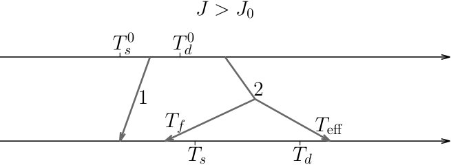 Figure 1
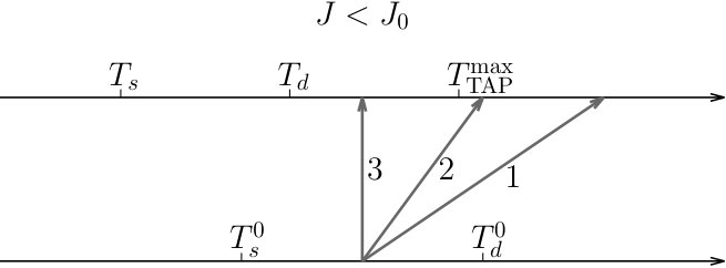 Figure 2
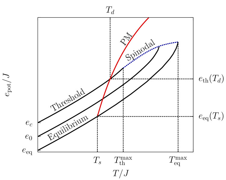 Figure 3
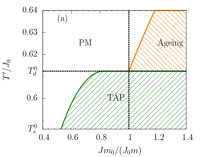 Figure 4
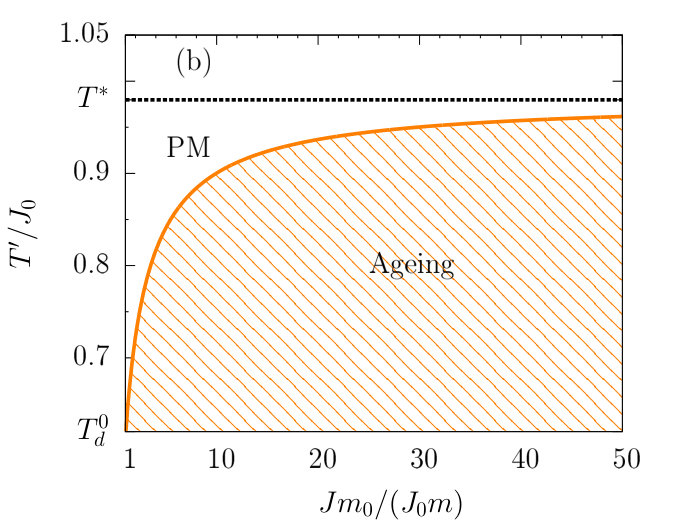 Figure 5
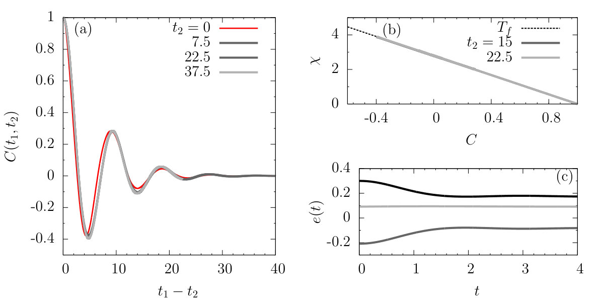 Figure 6
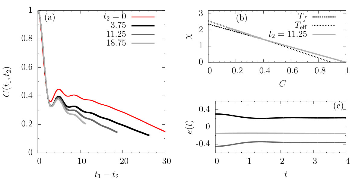 Figure 7
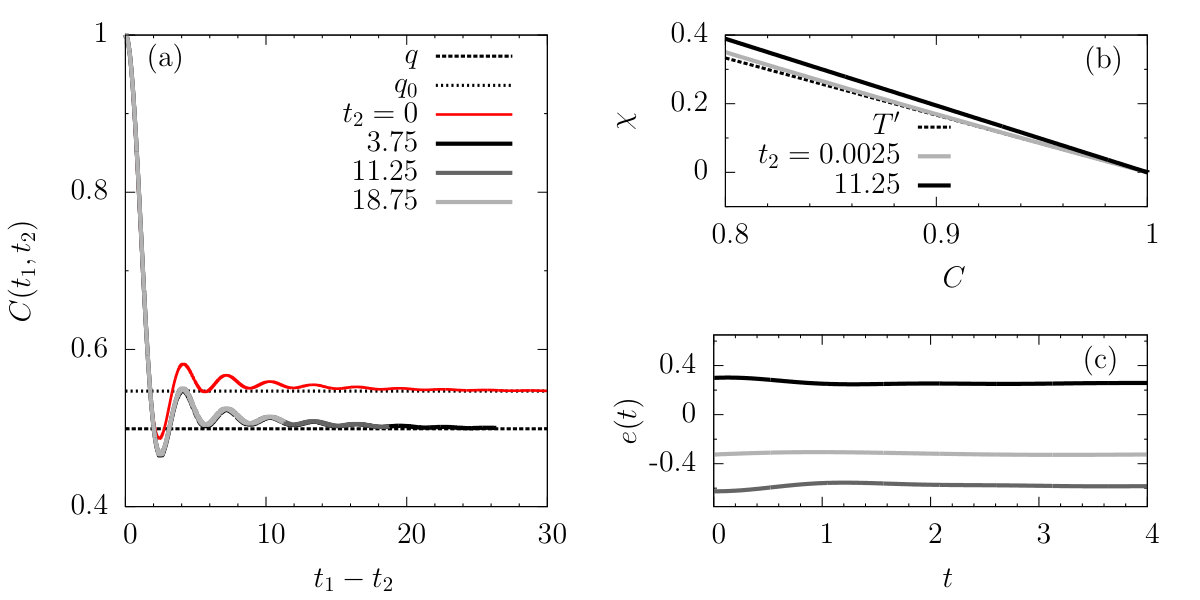 Figure 8
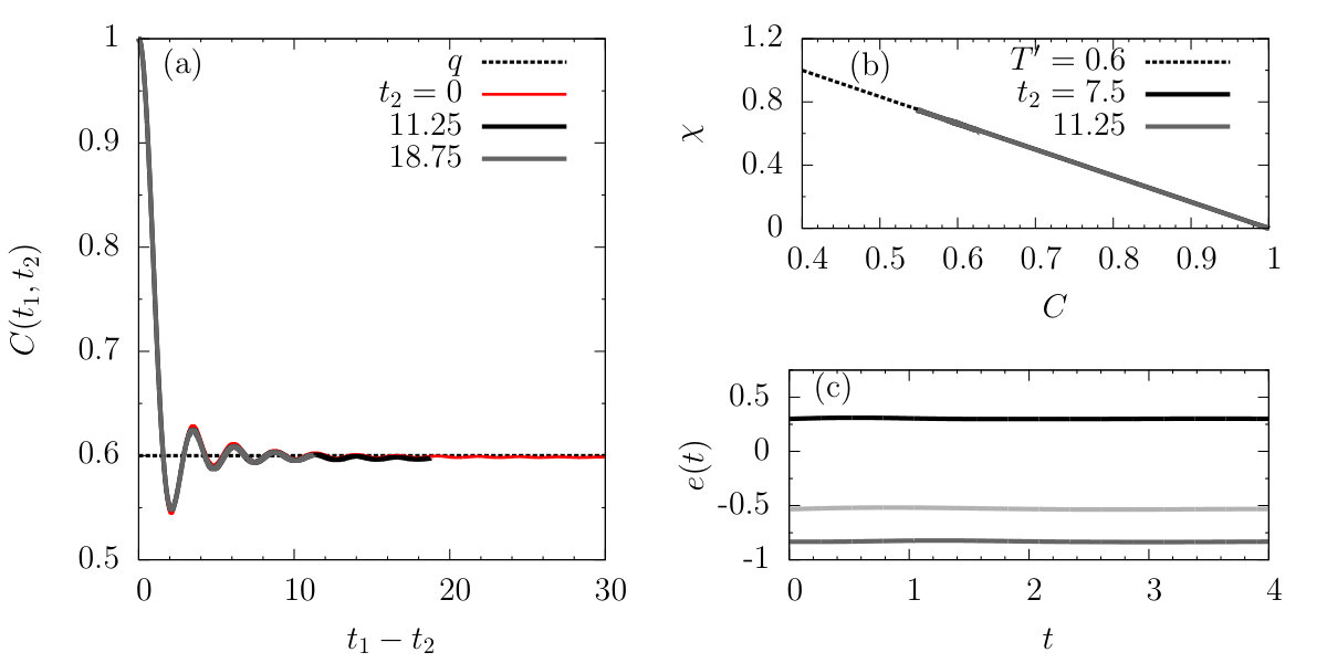 Figure 9
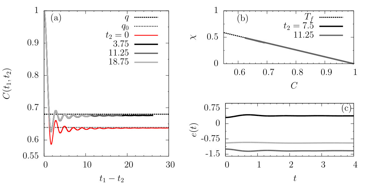 Figure 10
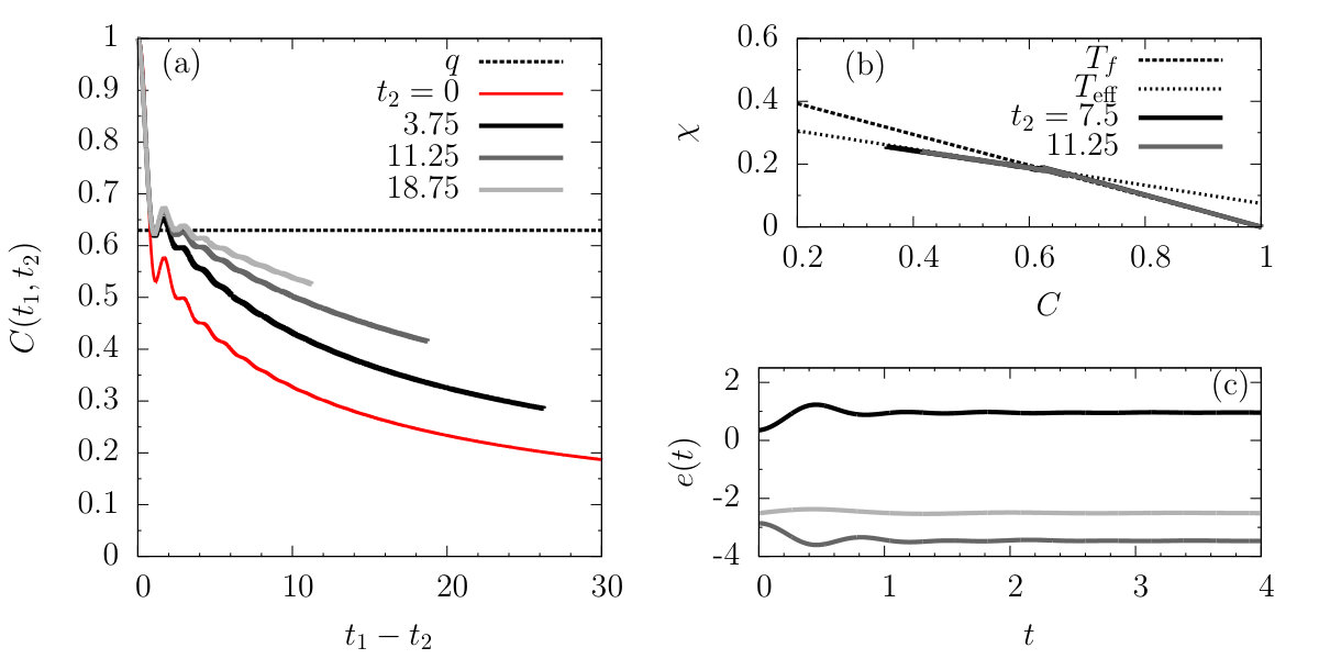 Figure 11
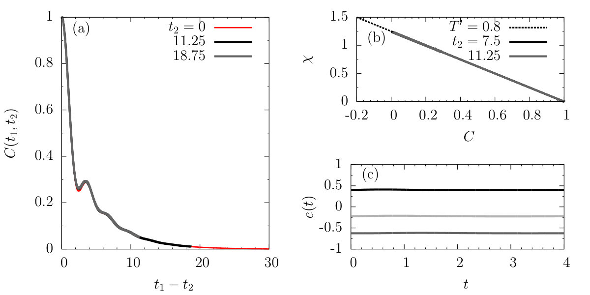 Figure 12
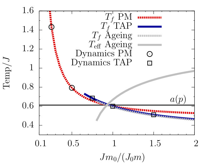 Figure 13
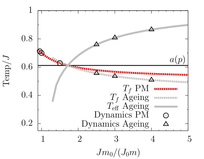 Figure 14
Peer Reviews
No public reviews on file for this paper yet. If you reviewed it on a platform where reviews are public (OpenReview, ICLR, NeurIPS, ICML), you can paste yours below so the community can read it here.
Videos
No videos yet. Explain this paper in a talk, walkthrough, or lecture? Add one.
Non equilibrium dynamics of isolated disordered systems:
the classical Hamiltonian p-spin model
Leticia F. Cugliandolo1, Gustavo S. Lozano2 and Nicolás Nessi2
1 Sorbonne Universités, Université Pierre et Marie Curie — Paris 6,
Laboratoire de Physique Théorique et Hautes Energies,
4, Place Jussieu, 75252 Paris Cedex 05, France
2 Departamento de Física,
FCEYN Universidad de Buenos Aires & IFIBA CONICET,
Pabellón 1 Ciudad Universitaria, 1428 Buenos Aires, Argentina
Abstract
We study the dynamics of a classical disordered macroscopic model completely isolated from the environment reproducing, in a classical setting, the “quantum quench” protocol. We show that, depending on the pre and post quench parameters the system approaches equilibrium, succeeding to act as a bath on itself, or remains out of equilibrium, in two different ways. In one of the latter, the system stays confined in a metastable state in which it undergoes stationary dynamics characterised by a single temperature. In the other, the system ages and its dynamics are characterised by two temperatures associated to observations made at short and long time differences (high and low frequencies). The parameter dependence of the asymptotic states is rationalised in terms of a dynamic phase diagram with one equilibrium and two out of equilibrium phases. Aspects of pre-thermalisation are observed and discussed. Similarities and differences with the dynamics of the dissipative model are also explained.
Contents
1 Introduction
The dynamics of isolated many-body quantum systems, and especially the search of a statistical description of their asymptotic evolution [1], are currently receiving much attention. One of the motivations to study these issues theoretically is the practical realisation of quenches of isolated ultra-cold atoms trapped in optical lattices [2]. Another reason for the interest in these questions, is the recently proposed many-body localisation phenomenon in systems with quenched disorder [3].
A quantum quench is the protocol whereby the ground state (or, more generally, a mixed state) of a Hamiltonian is unitarily evolved with a different Hamiltonian . A similar procedure can also be realised in a classical setting. It amounts to evolve an isolated system initially prepared in the equilibrium state (or, more generally, a metastable state) of a Hamiltonian with a Hamiltonian with the same form but different parameters. The latter problem has not received as much attention as the former although we will show that it raises very similar questions as its quantum partner.
The most natural question to pose in the context of quenches of isolated classical or quantum many-body physics is whether the system is able to provide a bath for itself, allowing it to reach equilibration thanks to the interactions. In other words, the question is whether the system attains, in the long time limit, a stationary state of Gibbs-Boltzmann thermal kind.
Two classes of quantum systems in which the answer to this question is negative have already been identified. These are integrable systems, with a macroscopic number of conserved quasi-local quantities [4], and many-body localised quantum systems, which remain localised in states that are close to their initial conditions forced by the frozen randomness [5, 6]. The non-ergodic behaviour of these systems is expected to be destabilised by the coupling to an external environment acting as a thermal bath [7].
Our aim is to prove that there exists another class of isolated non-ergodic models that are not able to act as baths for themselves. These are frustrated models with a complex free-energy landscapes that include, for wide ranges of variation of their parameters, fully trapping regions. For the sake of clarity, and with the aim of distinguishing effects that may be of unique quantum origin from features that are just due to the isolation of the model and/or the peculiar character of the interactions, we start by treating a classical model.
In this paper we start a series of studies of the quench dynamics of isolated classical and quantum interacting disordered models of mean-field kind, that is to say, models with fully-connected variables, endowed with a quenched random potential and kinetic energy. Their choice is motivated by the fact that their equilibrium, metastable and dissipative dynamics are very well understood and realise the complex free-energy landscape able to render the dynamics non-ergodic. Concretely, they are models with random interactions between spins that have been extensively used as a mean-field description of the glassy arrest and glassy phenomenology [8, 9, 10]. In the infinite limit they become the random energy model [11, 12], also used in the context of many-body localisation studies [13, 14].
We show that, under different quenching conditions, the isolated dynamics of these non-integrable interacting systems asymptotically approach:
- (i)
A paramagnetic stationary state described by a single temperature , itself determined by the final energy of the system . 2. (ii)
A metastable state with stationary dynamics. Whether this steady state can or cannot be considered one of Gibbs-Boltzmann equilibrium, is a subtle issue that we will explain in the paper. 3. (iii)
A non-stationary ageing state described by two temperatures, and , that are also related to the final energy of the system and other non-trivial properties of it. In this case, the system is clearly out of equilibrium.
The impossibility to relax to thermal equilibrium is related to two prominent features of the potential energy landscape. In case (ii), the system reaches stationarity within one (out of many) metastable state, which can be visualised as disconnected lakes in phase space. Provided that the quench does not change the energy landscape too drastically, any trajectory starting from initial conditions inside a lake will remain confined to it. The system will be unable to explore the whole phase space and, consequently, it will not reach a state compatible with thermal equilibrium. The case (iii), in which the system never reaches a stationary state, is related to the existence of the so-called threshold level, a region in phase space in which the potential energy is dominated by saddles points. Dynamics within the threshold level are characterised by slow relaxation and ageing.
We determine the dynamic phase diagram as a function of the pre and post quench parameters, with dynamic transitions lines and phases that we characterise. The behaviour found is robust against the coupling to a bath.
The paper is organised as follows. In Sec. 2 we introduce the model and we recall some of its main properties. Section 3 explains the quenches that we implement. In Sec. 4 we present the analytic developments and asymptotic results and in Sec. 5 we show the outcome of the numerical integration of the exact equations of motion. Section 6 presents the dynamic phase diagram. Finally, in Sec. 7 we present our conclusions and we briefly discuss our future projects.
2 Background
2.1 The Hamiltonian spherical -spin model
The -spin model is a model with interactions between spins mediated by quenched random couplings . The potential energy is [8, 9, 10, 11, 12]
[TABLE]
The coupling exchanges are independent identically distributed random variables taken from a Gaussian distribution with average and variance
[TABLE]
The parameter characterises the width of the Gaussian. In its standard spin-glass setting the spins are Ising variables. We will, instead, use continuous variables, with , globally forced to satisfy (on average) a spherical constraint, , with the total number of spins [15]. The spherical constraint is imposed on average by adding a term
[TABLE]
to the Hamiltonian, with a Lagrange multiplier. The spins thus defined do not have an intrinsic dynamics. In statistical physics applications their temporal evolution is given by the coupling to a thermal bath, via a Monte Carlo rule or a Langevin equation [16].
The model can be endowed with conservative dynamics if one changes the “spin” interpretation into a “particle” one by adding a kinetic energy [17, 18]
[TABLE]
to the potential energy. The total energy of the Hamiltonian spherical -spin model is then
[TABLE]
This model represents a particle constrained to move on an -dimensional hyper-sphere with radius . The position of the particle is given by an N-dimensional vector and its velocity by another -dimensional vector . The coordinates are globally constrained to lie, as a vector, on the hypersphere with radius . The velocity vector is, on average, perpendicular to , due to the spherical constraint. The parameter is the mass of the particle. The parameter is an integer and we will take it to be equal to in the numerical applications.
The potential energy (1) is one instance of a generic random potential with zero mean and correlations [19, 20, 21]
[TABLE]
with . The problem is also interesting for generic but we will focus here on the monomial case that corresponds to the -spin model. Details on the changes induced by other functions will be given elsewhere.
The generic set of equations of motion for the system coupled to a white bath is
[TABLE]
where the random force has a Gaussian distribution with zero mean and correlations , is the friction coefficient and is temperature. We have set, and we will keep, the Boltzmann constant to be . We have added the friction and noise terms to the Newton equation for completeness and to make contact with the stochastic setting usually used in the study of this model. Still, having introduced in Eq. (4) the kinetic energy that provides an intrinsic dynamics to the system, we will be able to switch off the coupling to the bath, that is to say set , and study the dynamics of the isolated system.
The initial condition will be taken to be and chosen in ways that we specify below.
2.2 The case
The spherical -spin model behaves very differently for and . Here we concentrate on the cases and we leave for a future study the model.
The model with has a very rich and complex free-energy landscape with interesting metastability. In the past, the model with just the potential energy was analysed in a considerable degree of detail. The kinetic energy allows one to study the dynamics of the isolated system without changing the picture of metastability described below, since it contributes a trivial Maxwell (Gaussian) factor to the canonical probability weight.
In short, the known results for the spherical model can be summarised as follows. In the thermodynamic limit, , the model has two “critical” temperatures . At high temperatures, , with the dynamical critical temperature, the equilibrium state is the paramagnetic one, with vanishing local order parameters. The analysis of the order-parameter dependent free-energy landscape proves that there is an exponentially large number of metastable states above the static critical temperature , (and until some high temperature ). Between and equilibrium is dominated by a class of metastable states that exist in exponentially large number (finite complexity). Below the number of metastable states is no longer exponential and the Gibbs-Boltzmann measure is dominated by the low lying ones. The dissipative relaxation dynamics of the model is consistent with the picture emerging from the static analysis. It is also surprising since for quenches from above to below the relaxation is non-stationary with ageing effects and other special features due to the fact that it occurs, asymptotically, on a flat region of phase space.
In the rest of this Section we turn the description in the previous paragraph quantitative. We give some details on how to derive the picture above with three methods: the replica trick, the Thouless-Anderson-Palmer (TAP) approach and the dissipative dynamics. We give the expressions for some characteristic temperatures and energies that will be useful in the study of the quench dynamics of the isolated system and we sum up, in Table 1, the values these take in the case.
2.2.1 Equilibrium
The static properties of a model with quenched randomness follow from the study of the disorder-averaged free-energy density in the canonical ensemble. The kinetic energy term in (4) is a conventional one and it does not depend on the quenched disordered interactions. The statistical sum over the velocities in the partition function can be readily performed and it yields the usual factor stemming from the Maxwell weight, . Instead, the contribution of the potential energy to the average over disorder of the logarithm of the partition function has been computed with the help of the replica trick [15]. In this framework one introduces an “overlap” matrix between replicas and () where the angular brackets denote the statistical average. In the case of the model, the one step replica symmetric Ansatz solves this problem exactly below in the limit. Within this Ansatz the matrix is parametrized as , with equal to one if are within a diagonal square block of size and zero otherwise. The parameters and are determined by requiring that they extremise the free-energy density calculated in the limit (after ).
The Edwards-Anderson parameter, , and the replica parameter, were derived in [15]. They are given, in implicit form, by the equations
[TABLE]
that are easy to solve numerically. In the limit, and with and .
The static transition temperature occurs at such that . This condition implies
[TABLE]
that in turn fixes to [15, 22, 23]
[TABLE]
Specializing to the case, . The phase transition is discontinuous, in the sense that the order parameter jumps at , and while above , and remains fixed to . The solution boils down, at high temperature, to a replica symmetric one. However, there are no jumps in the thermodynamic quantities so the transition is not of first order in this sense. It is a “random first order phase transition”.
The equilibrium potential energy density, , is then
[TABLE]
that simplifies to above and takes the value at for . At zero temperature the equilibrium potential energy is
[TABLE]
and at for .
Above the solution still exists (with ) and it disappears at a much higher temperature, , where
[TABLE]
For , .
2.2.2 Metastability
The Thouless-Anderson-Palmer (TAP) method serves to derive mean-field equations for the local order parameters, the local magnetisations,
[TABLE]
at fixed quenched disorder in the canonical ensemble. As everywhere in the paper, the angular brackets denote statistical average.
The TAP method also constructs the full free-energy and potential energy density landscapes. It has been applied to the study of the disordered -spin models landscapes in, e.g., [24, 25, 26]. The outcome for the potential energy as a function of temperature is summarised in Fig. 1. We explain the meaning of the different lines, and the special values of the potential energy and temperature highlighted in the figure, in the rest of this Subsubsection.
First of all, it is convenient to introduce
[TABLE]
and then observe that, for the spherical -spin model [25],
[TABLE]
due to the homogeneity of the potential energy. This property is not general and makes the structure of the potential energy landscape of the spherical -spin model particularly simple, with no level crossings nor birth of states at finite temperature, as sketched in Fig. 1. In other words, each state can be univocally labeled by its zero-temperature potential energy.
The extremisation conditions on the TAP free-energy lead to [25]
[TABLE]
with
[TABLE]
and the zero temperature energy. This equation admits real solutions for such that , with the threshold energy at zero temperature. Each of these solutions is an equilibrium or metastable state of the system. Equation (19) determines as a function of the energy density of a TAP solution at , , and temperature, , both measured in units of . In particular, one can check that replacing by as given by Eq. (14), the equation fixing the equilibrium Edwards-Anderson parameter, Eq. (9), is recovered. Otherwise, replacing by the equation for the threshold is obtained. The left-hand-side (l.h.s.) has a bell-shaped form with a maximum at . For the same equation determines above which the equation has no more solution. The physical solution is the one taking the largest value of , since it continuously connects to the zero-temperature one in which . Different TAP states cease to exist at different temperatures, as sketched in Fig. 1. The temperature at which this occurs for the equilibrium level is given in Eq. (15). The threshold level, instead, disappears at
[TABLE]
and for .
An expression of the potential energy as a function of and (itself a function of ) is
[TABLE]
Of particular interest is the threshold potential energy that we will give explicitly in Eq. (32).
The equation that fixes the values of the TAP states that combine (because of their macroscopic degeneracy) to yield equilibrium in the range is [25, 22]
[TABLE]
(These states have thermodynamic properties, like the internal energy, that coincide with the continuation of the high-temperature paramagnetic one. In the sketch in Fig. 1 these states correspond to points along the continuation of the PM line (red) inside the region where metastable states exist, i.e., the portion of the PM curve between and . Once again, the bell-shape form of the l.h.s. of Eq. (23) implies that this equation admits a solution for temperatures such that with
[TABLE]
were we have introduced the numerical constant
[TABLE]
that is smaller than for all .
We will recall the dynamic significance of these TAP states in the next Subsubsection. We announce here that and coincide with and , the critical dynamical temperature and the value of the parameter at this temperature. In particular, for , and at this temperature, .
The scenario with a large multiplicity of metastable states has been confirmed with the exhaustive enumeration of the extrema of the TAP potential energy landscape of finite (small) size spherical -spin models at fixed randomness [27].
2.2.3 Relaxation dynamics
The over-damped relaxation dynamics of the spherical -spin model (coupled to a Markovian bath) were studied in [16, 28]. The dynamics considered in these papers evolve a completely random initial condition, , that, for purely relaxational dynamics corresponds (formally) to an infinite temperature initial state. The latter is then quenched to a final state in contact with a bath at finite temperature . The analysis is performed in the thermodynamic limit, , and times are taken to infinity only after, remaining therefore finite with respect to .
For quenches with the dynamics quickly approach equilibrium at the new temperature. The correlation and linear response are invariant under translations of time and they are related by the fluctuation dissipation theorem.
Above but close to the relaxation exhibits a strong slowing down with the correlation decaying in two steps, with a first approach to a plateau and a further decay from this plateau, in a much longer time-scale, to zero. This is similar to what is observed in super-cooled liquids and it is the reason why this model has been used as a toy model for glass formers of fragile kind.
For , the evolution of the correlation and linear response functions conform to the weak-egodicity breaking scenario [16, 28] in which they separate in two contributions evolving in different two-time regimes
[TABLE]
with the stationary and a non-stationary terms linked by the fluctuation-dissipation theorem (FDT) at the temperature of the bath and a modified FDT at an effective temperature [29, 30] selected by the dynamics,
[TABLE]
always with . In the asymptotic limit, the two terms added to form and evolve in different regimes in the sense that when one changes the other one is constant and vice versa. The limiting values of the various contributions to the correlation function are
[TABLE]
with being equal to , the value at the threshold of the TAP free-energy density.
The asymptotic potential energy reached after the quench for is the one of the threshold level in the free-energy landscape:
[TABLE]
This expression will be very useful in the numerical analysis. The parameters and are given by
[TABLE]
The parameter measures the violation of the fluctuation-dissipation theorem out of equilibrium and can be interpreted in terms of an effective temperature [29] (note that and for quenches from high to low temperature).
The bell-shaped function in the l.h.s. of Eq. (33) indicates, once again, that this equation has two solutions until a temperature given by the same expression, Eq. (21), obtained with the TAP formalism. The relevant solution is the one taking the higher value, the one that is connected to at . Its value and the energy at this temperature are given in the Table that accompanies Fig. 1.
The equation fixing as a function of is implicit so we cannot write an explicit expression for . We can, instead, eliminate from Eq. (32) using Eqs. (33) and (34), and then recast Eq. (32) as
[TABLE]
At , with and . Expanding in powers of one finds and then
[TABLE]
as expected. Its concrete value for is given in Table 1.
The dynamic critical temperature arises when :
[TABLE]
that coincides with Eq. (24). Specialising to the case . When this occurs and .
The dynamic relevance of the TAP states that are non trivial but “confused” with the paramagnetic solution with the conventional replica calculation, the ones with values determined by Eq. (23), is understood from the analysis of the relaxation dynamics starting from initial conditions in equilibrium at the range of temperature [31, 32, 33, 34]. These initial conditions are confined within TAP states that do not let the system escape. The asymptotic dynamics remain within the departing state, as indicated by the fact that , with given by Eq. (23).
For finite the threshold level dynamics and evolution within TAP states should have finite, though exponentially large in , lifetime. Some numerical evidence for this was given in, e.g., [35, 36, 37].
3 Quenches and dynamics of the isolated system
The Hamiltonian (5) with and given in Eqs. (4) and (1) has two parameters, the variance of the couplings and the mass of the particle. We will consider initial conditions sampled from equilibrium at with Hamiltonian and evolve them with a different Hamiltonian . Since the potential and kinetic energies play different roles, as the former depends on the quenched randomness while the latter does not, the treatment of the quenches induced by a change in the random interactions needs a bit more care.
Let us take the -spin model (1) and (4) with coupling constants in canonical equilibrium at temperature and evolve it in isolation from the environment with a modified Hamiltonian. Quenches in the random exchanges that do not keep any memory of the values before the quench are not interesting. We therefore impose quenches in the potential energy such that each random choice of the exchanges is changed into , with the new couplings related to the old ones by
[TABLE]
This transformation is such that for each sample (disorder realisation) at we uniformly change the value of all random couplings by the same factor. In other words, we prepare the system in a thermal state of a Hamiltonian with potential energy
[TABLE]
but let each initial condition sampled from this state evolve with the Hamiltonian with potential energy
[TABLE]
Note that with we enhance the interactions and with we depress the interactions between the spins. Technically, after relating the coupling strengths one by one we have only one quenched disorder average to make.
It is important to note that under this change, the potential energy levels in Fig. 1 are translated upwards or downwards, and stretched or contracted, for or , respectively. Indeed, one can easily see the translation by noticing that is proportional to , and the contraction by noticing that the various are proportional to . Concomitantly, the static and dynamic critical temperatures and of the initial potential are shifted to new values and after the quench,
[TABLE]
We will also consider quenches in the mass, , that change the kinetic contribution to the energy as
[TABLE]
3.1 Dynamical equations
Importantly enough, all our results will be derived after having taken the limit from the start, and eventually considering the long-times asymptotic limit only after.
In the limit the dynamics of the model are fully characterised by the behaviour of the two-time correlation and linear response function. The equations ruling their evolution are easily derived using the Martin-Siggia-Rose functional formalism.
Particular initial conditions can be imposed by including in the dynamic generating function an integration over the initial conditions weighted with their distribution. Equilibrium initial conditions at a temperature are distributed according to the Gibbs-Boltzmann measure
[TABLE]
with defined in Eqs. (1)-(5). The Hamiltonian depends on the quenched random interactions. The average over disorder in the case of initial states correlated with the quenched randomness needs the use of the replica trick, as explained in Ref. [31]. This means that the spin variables evaluated at the initial time have to be replicated, , with , to perform the average over the random exchanges. The subsequent evolution of each of these replicas has to be followed in time, and it turns out that the replica structure of the initial condition is conserved.
For the dissipative spherical -spin model this calculation has been carried out in [33, 34], and it can be adapted to the isolated model with kinetic energy with just minor modifications. We therefore present the outcome here without giving many details of the derivation. In order to facilitate the comparison to the expressions for the dissipative model we keep the coupling to the white bath active in the presentation of the dynamic equations. Later on, we will focus on the isolated problem.
In the limit, the only relevant correlation and linear response functions that determine the dynamics of the model are
[TABLE]
for , where the infinitesimal perturbation is coupled linearly to the spin at time and the upperscript indicates that the configuration is measured after having applied the field . The square brackets denote here and everywhere in the paper the average over quenched disorder. The angular brackets indicate the average over thermal noise if the system is coupled to an environment, and over the initial conditions of the dynamics sampled with the probability distribution . When the coupling to the bath is set to zero, , the last average is the only one remaining in the angular brackets operation.
Without loss of generality we will focus on initial states in equilibrium at , where the replica structure is symmetric, although there can still be a complex structure of metastable states, as explained in Sec. 2.2.2. Considering the case would add quite a lot of unnecessary complexity to the calculations, while we do not expect major changes in the dynamic behaviour under such initial conditions. For these reasons, the following expressions are valid only for .
The dynamical equations of the model coupled to a bath at temperature , starting from a random state, are well known and can be found in Refs. [16, 22, 23, 28]. They can be derived from the dynamical Martin-Siggia-Rose action
[TABLE]
where the subscript in indicates that the action depends explicitly on the disordered couplings and the are (imaginary) auxiliary variables used to rewrite a delta function that enforces the validity of the equation of motion in the path integral. (This form corresponds to the Ito convention in which there is no Jacobian contribution.) We included here the kinetic energy contribution not present in these publications.
The replicated dynamical action that includes the contribution from the distribution of the initial conditions reads
[TABLE]
The kinetic energy term in the initial distribution does not depend on the quenched random interactions, it does not affect the dynamic equations, but will appear only in the energetic considerations that we will develop below.
We will now show how to perform the average over the couplings in some detail. Two terms in (46) depend on the interactions, they are the ones in which appears in the force in the evolution equation and in the initial contribution . We collect them in . (Note that we use, as a working assumption, that does not depend on .) The average over disorder of the exponentials of these two terms is
[TABLE]
where we have included the Gaussian distribution over the couplings (we average over the final couplings but the same results would be obtained had we chosen to average over the initial ones, ). We have symmetrised the term originating in . Following our choice of quench we set , in which case the disorder dependent part of the action becomes
[TABLE]
After performing the Gaussian integration over the couplings we have
[TABLE]
The product between the two terms involving integrals in time produces the terms already present in the dynamical equations starting from a random initial condition. These terms are proportional to . The product between a term with one time integral and one term with the initial condition generates the new terms. They are proportional to , that is to say , if we call . The product of the terms involving only the initial conditions yields the equilibrium equations of the model decoupled from the dynamics, and are proportional to , as they should.
Taking now one derives the dynamical equations that read
[TABLE]
One can check that these equations coincide with the ones in [33, 34] when inertia is neglected and .
In the rest of the paper we switch off the connection to the environment by setting . With inertia and no coupled bath, the equal-time conditions are
[TABLE]
for all times larger than , when the dynamics start.
3.2 The Lagrange multiplier
We found convenient to numerically integrate the integro-differential equations that determine the time-evolution of the system to use an expression of the Lagrange multiplier that trades the second-time derivative of the correlation function into the total conserved energy after the quench. More precisely, we proceeded as explained below.
Firstly, we provide an expression for the kinetic energy density,
[TABLE]
Using the definition of , and the fact that, for sufficiently short time differences it is always possible to write , with , we find that
[TABLE]
On the other hand, the potential energy is linked to the kinetic energy and the Lagrange multiplier via a general equation proven as follows. Take the microscopic evolution of , multiply it by , and take the average over initial conditions:
[TABLE]
Summing now over , normalising by , and taking the limit ,
[TABLE]
This implies that
[TABLE]
The two contributions added together yield the total energy density of the system
[TABLE]
conserved after the quench.
Rearranging now the equation for , Eq. (58), with the help of Eq. (56), we obtain a new expression for the Lagrange multiplier
[TABLE]
Using now the original equation for , Eq. (52), we can eliminate the second time derivative to obtain
[TABLE]
It seems that we have simply traded by . However, for an isolated system , a constant. Then, the last expression allows a straightforward numerical solution of the evolution equations for the isolated system since it does not involve the second time derivative of the correlation function. In practice, in the numerical algorithm we fix the total energy and we then integrate the set of coupled integro-differential equations with a standard Runge-Kutta method. We only have to define which is the total energy density of the system, the subject of the next two subsections.
3.3 Energy change
We now determine the energy changes induced by a quench in the disorder exchanges and a quench in the mass of the particle. As these two act separately on the potential and kinetic contributions to the total energy, the total energy change is the sum of the two variations.
3.3.1 The energy change after a potential energy quench
Let us investigate what is the change in energy density induced by the change in potential energy , while keeping the mass constant .
The energy density just before the quench is the energy density of a canonical equilibrium paramagnetic state at temperature and it is given by
[TABLE]
The first term is the equipartition of the kinetic energy and the second one is the potential energy of the paramagnet in equilibrium. Note that this is still true if we choose , since, although metastable states still dominate the energy landscape in that range of temperatures, the thermodynamics of the equilibrium states is indistinguishable from the one of the paramagnet (see Section 2.2.2).
The energy density at time right after the instantaneous quench is
[TABLE]
Using the fact that with no mass change the kinetic energy does not vary between and
[TABLE]
as confirmed numerically in Sec. 5, and the value of the Lagrange multiplier evaluated from Eq. (52) at is
[TABLE]
we find
[TABLE]
Equations (60) and (61) imply that the amount of energy injected during the instantaneous quench is
[TABLE]
Therefore, if and if .
3.3.2 The energy change after a quench in the mass
If we apply a quench in the mass, , while leaving the random exchanges fixed, the energy balance is modified.
Imagine that we initialise the system in a paramagnetic or TAP state such that . If we change the mass according to , the potential energy does not change during the instantaneous quench. Instead, the kinetic energy does. Right before the quench the kinetic energy density is
[TABLE]
while right after the quench the velocities have not changed but the mass of the particle has. Therefore,
[TABLE]
The total energy after the quench is
[TABLE]
and the energy input by the quench reads
[TABLE]
Adding together the energy variation due to the the potential and mass quenches, the total energy change becomes
[TABLE]
4 Asymptotic analysis
Depending on the pre and post quench parameters the system reaches different asymptotic dynamics. In some cases, the system reaches a stationary regime but, for parameters carefully tuned, a final state with non stationary ageing behaviour can also be attained.
Before entering into the deduction of the asymptotic equations, we present the general reasoning that we use to find them.
We will first analyse in Sec. 4.1 the cases in which a stationary regime is reached after the quench. This means that
-
We assume time-translational invariance (TTI) , with and
-
the fluctuation-dissipation theorem for .
-
We define the asymptotic limits of the correlation with the initial configuration ,
-
and between two dynamic configurations .
-
We assume that the kinetic energy density approaches after the quench.
Clearly, all these assumptions can and have been verified numerically. The temperature of the final state, , has to be calculated and the parameters and as well.
We anticipate that the parameters and will find two interesting interpretations in the cases in which the system is initially in a non-trivial TAP state. The value represents the overlap between a typical configuration of the TAP state of the pre-quench potential in which the system was prepared initially, and a typical configuration of the TAP state into which the original state has evolved in the post quench potential, if it still exists. Instead, is the self-overlap within the TAP state of the post-quench potential. This description will become clear after presenting the analytical and numerical results.
We will then analyse, in Sec. 4.2, the cases in which the system, starting from equilibrium in a disordered paramagnetic state at high temperature is set, after the quench, on the threshold level and the stationarity assumption fails. This is in agreement with what was expected from the properties of the states on the threshold, that are flat, and on which ageing properties were obtained after quenches from random initial conditions in the dissipative setting [16, 28]. For these cases we need to modify the assumptions above and allow for a two-time scale dependence of the correlation and linear response functions that take a form with a separation of time-scales, as in Eqs. (26) and (27). This Ansatz is introduced in the dynamic equations for and , Eqs. (50)-(52), and the evolution in two two-time sectors is studied separately together with the requirement that the behaviour matches in the crossover region. The resulting equations are manipulated a bit, and equations for the parameters , and , are derived. We reckon that with this procedure we introduce three unknowns and we deduce five equations, one being the energy conservation. The other four equations are the equations for , , and , but these are not all independent, since the FDT with for (, ) and for , ) reduce their number to two. There are then three unknowns and three equations.
4.1 Stationary dynamics
In this Section we derive the set of equations that determine and as a function of the properties of the initial state, , and , and the ones after the quench, and , assuming that a stationary state is reached.
The stationarity assumption implies
[TABLE]
where we took . The large limit can then be further considered to define
[TABLE]
This asymptotic limit has to be distinguished from the one of the correlation between the initial condition and the dynamic configuration
[TABLE]
The parameters and will take zero or non-vanishing values in different situations presented below. Accordingly, since in the former equation the limit has been taken and in the latter equation . In the following presentation we drop the superscript from the initial time but the [math] of the absolute times should be understood as .
If and satisfy FDT with respect to a temperature , and we call ,
[TABLE]
where we used . The second way of writing the FDT is the one that we will exploit in the numerical analysis to determine the final temperature from the plot of against constructed using the time-lag as a parameter.
In order to make the presentation of the analytic part easier we list here the steps followed in the derivation of the asymptotic equations under the stationary assumption:
- We take the asymptotic limit of the equation for and write as a function of the
and parameters and .
-
We write the conservation of the energy.
-
We prove that the equation for becomes the -derivative of the equation.
-
We take the asymptotic limit of the equations for and .
The conservation of the total energy and the two last equations derived constitute a set that fixes , and knowing , , , and . We do not prove analytically that the asymptotic solution is reached by the dynamics, this would need the full solution of the equations of motion and a matching problem that remains out of reach analytically. In contrast, we do verify a posteriori for which set of parameters this occurs by solving numerically the full set of equations.
The steps followed in the case in which the system ages and stationarity is broken are rather similar but need some generalisation, see Sec. 4.2.
4.1.1 The asymptotic Lagrange multiplier and the total energy
Starting from Eq. (59) and using FDT
[TABLE]
the integral can be computed and an asymptotic expression for is obtained
[TABLE]
Proceeding similarly, the potential energy is given by
[TABLE]
that becomes the paramagnetic result for . Moreover, if and (no potential energy quench), and , independently of , as it should. Note that we need the contribution from the last term to get the correct no-quench limit. Besides, we assume that the asymptotic kinetic energy is determined by “equipartition” at the final temperature
[TABLE]
Then, the asymptotic total energy reads
[TABLE]
We argued that the energy right after a quench in the interactions and mass is . Compared to the asymptotic form derived in Eq. (75) the conservation of the total energy implies
[TABLE]
We see here two adimensional parameters and that characterise the pre-quench conditions and the comparison between the pre and post quench parameters.
The equation for in Eq. (72) can now be rewritten as
[TABLE]
after replacing the energy by its dependence on . It takes now a form that is very similar to the one of the relaxation dynamics [16].
4.1.2 The asymptotic analysis of the correlation equation
The equation for can be treated in two regimes of times. In one case we take fixed and and tending to infinity. The equation for then reads
[TABLE]
When deriving this equation we assumed that the contribution to the integrals of any possible transient between the time [math] and a time after which the FDT establishes can be neglected. The lower limit [math] in the integral over is then to be interpreted as the initial time of this asymptotic regime, although we simply write [math] in these equations. In the second integral [math] is the minimal time-delay at which the functions and are measured.
We can treat in the same way the equation for and then compare the two. As already mentioned in the list that summarizes the steps to follow, we can prove that the equation for is the time-delay derivative of the equation for times . This is a quite straightforward calculation that we choose not to show here.
In the limit we can replace and by . We further take the limit and drop the second time derivative assuming that the dynamics become slow at long time delays. The first integral is computed as it is written now. The second one is made more symmetric before approximating it, in such a way that the two extremes ([math] and ) contribute in the same way. One has
[TABLE]
Finally,
[TABLE]
This equation admits the solution but it can also have, for certain values of the parameters, solutions with and being equal or different.
The other interesting limit is the one in which we set to be strictly [math] and we tend to infinity. The equation for becomes
[TABLE]
In the limit we can replace by and use . We further drop the second time derivative, and use stationarity and FDT, to find
[TABLE]
This equation admits the solution but it can also have, for certain values of the parameters, solutions with . As a check of consistency, we remark that for and the two remaining equations, Eqs. (80) and (82), are compatible for .
We can now write down two other equations that relate and :
[TABLE]
4.1.3 The equations fixing the parameters , and
After some rearrangements, the three equations (76), (83) and (84) simplify to
[TABLE]
One can use Eqs. (85), (86) and (87) to determine in situations in which a steady state is reached.
More simplifications are possible if one extracts from the second equation and inserts it in the third one to obtain
[TABLE]
a linear equation in .
We can now check that for and , the equation that expresses energy conservation is consistent with and . Moreover, taking , Eqs. (87) and (88) become the same one,
[TABLE]
that is the equation for in the TAP solutions that are mixed to yield the non-trivial paramagnet at , see Eq. (23). The dynamics remain confined in the initial TAP state where the system was prepared.
4.1.4 Quench dynamics, target paramagnetic state
Let us look for solutions with that correspond to a final paramagnetic state. Equations (86) and (87) are identical to zero and Eq. (85) implies
[TABLE]
that fixes
[TABLE]
As the temperature cannot be negative, the plus sign is the relevant one here. This relation can be used to check whether the system has really attained thermal equilibrium by looking at the parametric plot of the integrated linear response, , as a function of the correlation function, , and comparing minus the inverse slope with . For a stationary system, the expected linear form is given in Eq. (70).
The temperature in the asymptotic paramagnetic state, in units of , is a function of and . One can easily show from the analytic form above that at . In the limit the temperature approaches . If, moreover, also diverges, it becomes . Some special finite values are for , and if and .
The curve as a function of the full control parameter is shown with dotted blue lines in the two panels in Fig. 2 that represent quenches from equilibrium at and . The open circles correspond to dynamical runs that realise the paramagnetic asymptotic solution. We will discuss the region of parameters in which this is the asymptotic state in Secs. 5 and 6.
The relation between the final total energy and the final temperature is very simple in the paramagnetic state
[TABLE]
and it coincides with the result of inverting Eq. (60), that is to say, the equilibrium paramagnetic energy as a function of temperature.
4.1.5 Dynamics within metastable states
When the temperature of the initial condition is such that , the system is prepared in a TAP state. In this Section we will show that whenever the asymptotic equations (85)–(87) have solutions with , the dynamics of the system are confined to the same TAP state that, after the change in the coupling strength operated at the quench, is only translated in the potential energy landscape and possibly rescaled in size, thanks to the fact that in the spherical -spin model there is no birth, death or merging of states at intermediate temperatures.
The first remark is that, as already mentioned, the interaction quench changes the depth of the potential energy minima. If one minimum has energy initially, its energy after the quench is given by
[TABLE]
Given that , the initial state is described by Eq. (23) that we here rewrite making the dependence of the parameter on the initial temperature, , and strength of the random potential, ,
[TABLE]
explicit. Indeed, is the equilibrium value of the self overlap at the initial temperature . This equation can be written in a slightly different way that will be useful later
[TABLE]
We call the bare potential energy of the TAP state that dominates the partition function at the initial temperature . In such case, from Eq. (19), also fullfills
[TABLE]
where . According to Eq. (93), after the quench, the energy of this TAP state is given by .
Let us call the self overlap in the final TAP state at temperature . Also from Eq. (19), and since the energy of the TAP state is rescaled, it is clear that satisfies
[TABLE]
where . Recalling that , we can write
[TABLE]
Then, from Eqs. (94), (96) and (98) we obtain a relation between and
[TABLE]
Using now the results for the asymptotic analysis of the dynamical equation, more precisely, Eqs. (87) and (88), the equation for can be written as
[TABLE]
Defining
[TABLE]
we can write Eq. (100) as
[TABLE]
Comparing this last equation with Eq. (95) we conclude that
[TABLE]
which, using Eq. (99), implies
[TABLE]
This shows that the system remains trapped in the same metastable state during all the evolution. Of course, if the quench takes the system to parameters (final temperature ) such that this state does no longer exist, the system escapes it into the proper paramagnetic state.
In Fig. 2 (b) we draw, with blue dotted lines, the dependence of for the asymptotic TAP states and the open squares show the numerical solution of the full equations for two choices of that realise this asymptotic state.
4.2 Non stationary dynamics and ageing
Let us now explain how the ageing equations are studied. In the aging regime we expect the correlation with the initial configuration to decay to zero
[TABLE]
The dynamic equations (50)-(52) therefore lose the terms that depend on the initial conditions. The only formal difference with the equations for the dissipative case [16, 22] is that the friction term (first time derivative) is now replaced by the inertial term (second-time derivative) and that the temperature is not fixed a priori.
4.2.1 The parameters , , and
Following the explanation in [16], explained in more detail in [38], the study of the and yields the equation that fixes plateau parameter to be the one on the threshold, Eq. (33). In the stationary regime the temperature is given by the parameter in the FDT linking and , that is not fixed yet. Moreover, the combination of the and equations in the stationary and aging regime yields the equation that fixes the effective temperature in the aging regime, , and this equation is, again, the same as in the dissipative case, Eq. (34). We have
[TABLE]
It is not necessary to fix the value of the Lagrange multiplier to derive these two equations. We still need to find, though, which is the value of selected by the closed system.
The selection of is done by the energy conservation. The asymptotic energy is the sum of the kinetic contribution, , and the potential one that reads
[TABLE]
Therefore
[TABLE]
We now have three equations for the three unknowns and . These equations can be simplified and recast in a more convenient manner by replacing the -dependence of from Eq. (107) in Eq. (109), that is now a quadratic equation on . Solving for and replacing the result in Eq. (106), after a straightforward calculation, we obtain
[TABLE]
Equation (110) determines given the initial temperature , the pre and post quench variance of the random interactions parametrized by and and the pre and post quench masses and . These parameters appear in the combinations and . Once is found, Eqs. (106) and (107) yield and , respectively.
The solutions to Eq. (110) can be understood graphically. The r.h.s. is a function of with positive curvature and a single minimum at , the overlap at the spinodal, in the interval . The equation has two solutions, the one with larger value being the relevant one. When the control parameter is decreased, the equation ceases to have solution at
[TABLE]
when the l.h.s. touches the minimum of the r.h.s. This value is for and for , and (see the ending points of the ageing and curves in Fig. 2, and the discussion of the phase diagram in Sec. 6).
In the ageing solutions, as long as (the temperature of the fast degrees of freedom) is lower than , the effective temperature is larger than . When goes beyond , its relation with the effective temperature is inverted, and it becomes larger than :
[TABLE]
The curves of and , as functions of are shown in Fig. 2 with solid grey and dotted grey lines, respectively. The open triangles indicate the actual solution of the full equations found numerically. The temperature inversion, predicted by the asymptotic ageing equations for is not realised asymptotically by the full equations but, as we will show in Sec. 5.2.3, it appears in a transient regime.
4.3 Summary of asymptotic solutions
As a summary of the different asymptotic solutions, we show in Fig. 2 the -dependence of the dynamic critical temperature, from Eq. (37), the final temperature of the PM () and TAP () branches of the solutions to Eqs. (85)–(87) (stationary Ansatze), and the final temperature, , and effective temperature, , derived from the solution to the set of equations (106)-(110) (ageing Ansatze). We note that the ageing temperatures and coincide with at a single value of the control parameter . We also show with different points the results from the full solution of the evolution equations, indicating which is the asymptotic solution realised by the dynamics in each range of parameters.
In panel (a), the initial state is paramagnetic , and the dynamics choose the PM solution (red dotted line and open triangles) for energy injection or for small energy extraction, while for sufficiently large energy extraction the asymptotic dynamics show ageing, characterised by two temperatures (grey lines).
In panel (b), and the initial configurations are drawn within a TAP state. The dynamics choose the PM solution (red dotted) for large energy injection, while the system remains in a TAP state (blue lines and open triangles) for small energy injection or for energy extraction. The ageing solution (grey lines) are not realised by the dynamics.
The exact boundaries between the different kinds of solutions selected by the full equations will be derived analytically in Sec. 6. In general, transients appear in the parameter regions where the system changes its asymptotic behavior.
5 Numerical results
In the numerical solution of the full set of equations we fix . This means that the initial energy landscape is fixed. In particular, we know the values of the initial critical temperatures and . We shall then vary the initial temperature and the coupling of the Hamiltonian that drives the time evolution.
For later reference and recalling the discussion in Sec. 3, the critical temperatures corresponding to the equilibrium landscape with the final coupling can be calculated by noticing that the critical temperatures are proportional to the coupling. Then
[TABLE]
After some general considerations about the numerical algorithm we analyse some specific processes to illustrate the analytical results of the previous Section and put them to the test. We will consider energy injection and energy extraction processes sketched in Figs. 10 and 11, respectively. The full numerical solution to the equations allows to prove which among the asymptotic solutions are realised, when several co-exist.
5.1 Equilibrium dynamics
We first checked that for and , that is to say , the system has a stationary evolution for all equilibrium initial conditions.
We studied the no energy change case with two purposes. One is to check consistency of our numerical algorithm. The other is to investigate the effect of the discretisation step on the results obtained from the numerical integration of the equations. We found that the algorithm does conserve energy and that a step was sufficient to assure numerical convergence of our results.
We used two typical cases as initial states, a paramagnetic configuration and a metastable TAP state. Figures 3 and 4 show three plots, with the dynamics of the correlation function (a), the fluctuation dissipation parametric plot (b) and the two contributions to the energy and the total energy (c), starting from equilibrium at and , respectively. In both cases the system is paramagnetic initially, though at it is a proper paramagnet while at it is a paramagnet-looking state made of a mixture of non-trivial metastable states, see Sec. 2.
Let us first focus on Fig. 3. The correlation with the initial condition, (thin red line) and the ones between two different times (grey lines) lines are identical, apart from a small deviation at short time-delays, around the first oscillation. The two-time correlation function is invariant under time-translations, that is to say, it is a function of only. All the correlation functions relax to zero, (a). The Lagrange multiplier (not shown) and the potential and kinetic energies (c) quickly approach their final values and these agree with the ones predicted analytically. The fluctuation-dissipation relation is satisfied with the temperature of the initial condition, that is the same as the one of the final state (b). All these results are compatible with equilibrium in the paramagnetic phase.
In Fig. 4 we show results for . The Lagrange multiplier (not shown) and energy densities approach constants (c), and stationarity is satisfied as well as the FDT with the initial temperature (b). The main difference with the case is that the correlation functions, both with the initial condition and with the configuration at a waiting-time , relax to a non-vanishing value (a). Within numerical accuracy we observe and this value as well as the asymptotic potential and kinetic energies are consistent with the ones stemming from the analysis in Sec. 4.1.2. One can use Eq. (89), that coincides with Eq. (23) and fixes the values of the non-trivial TAP states that correspond to equilibrium in the interval [25], and check that the solution for is , the value obtained with the numerical solution of the full dynamic equations. As regards the energy values, the kinetic energy should be that is obtained numerically. The potential energy is expected to be which is also correct numerically. These values are added to , as they should.
5.2 Energy injection
In this subsection we explore the dynamics after energy injection ( and ) and we compare our results with those obtained analytically in the previous Section.
The injection of energy over an initial state with temperature trivially evolves into a paramagnetic state at a temperature . The temperature can be calculated from the conservation of energy and the fact that for the PM phase . It is given by Eq. (91). We have checked that the numerical solution complies with these claims (not shown here). Therefore, we shall focus on the more interesting cases with initial temperatures such that . Figure 10 summarises the results of the concrete numerical quenches with energy injection that we display.
5.2.1 : from TAP to PM
In Fig. 5 we show results for , and . The system is initialised in a TAP state that corresponds to equilibrium between and , see Section 2.2.2. This quench injects a large amount of energy in the system . The system is initialised in a TAP state that corresponds to equilibrium between and , see Section 2.2.2.The post-quench critical temperatures are and . The self correlations shown in (a) rapidly decay to zero for all reference times, either when they correspond to an initial or to a waiting-time . Therefore . These facts indicate that the system behaves as in the paramagnetic state after the quench. The final temperature predicted by the asymptotic analysis, Eq. (91), is in very good agreement with the numerical result extracted from the parametric plot in (b). Considering the results from Section 4.1.5 for quenches starting from a TAP state it is important to know the temperature at which the initial TAP state ceases to exist, i.e. the position of the spinodal line in the post quench energy landscape (see Fig. 1). For and , . Note that which is consistent with the system reaching a paramagnetic state with , although it was initialised in a non-ergodic initial state, since for that final temperature the TAP state no longer exists. From the energetic dynamics (c) we observe and , both results consistent with equilibration in a paramagnetic final state. At very short times, , the energies are the ones right after the quench, and . It is only after a short transient, , that the energy densities converge to their final values.
5.2.2 : from TAP to TAP
In Fig. 6 we show results for and . This quench injects a smaller amount of energy into the system . The post-quench critical temperatures are and . Differently from the previous case, the correlations with the initial time and with a waiting time decay to non-vanishing values, and , respectively. The asymptotic analysis condensed in the full set of Eqs. (85)–(87) predicts and that are in very good agreement with the values obtained with the numerical solution of the dynamic equations shown in (a).
In panel (b) we display the parametric plot for a long waiting time , that finds good agreement with the FDT at the final temperature predicted by the asymptotic analysis. As a complement we also plot the parametric construction for a very short waiting time, , to demonstrate that, for very close to one, the slope is determined by the initial temperature instead of . It is only after a transient that the FDT with the final temperature establishes.
The results in the previous paragraph are consistent with the fact that the energies reach their asymptotic values only after a (short) transient. From the energetic dynamics we observe that after and, , measured after the same transient, is also in very good agreement with the predictions of the asymptotic analysis, once the non-vanishing values of and are taken into account.
The temperature at which the TAP state in which the system was initialised, modified by the quench, disappears is , that is slightly above the final temperature . Consequently, the analysis in Sec. 4.1.5 applies to this case and, after the quench, the system follows the TAP state in which it was set in initially.
5.2.3 : from TAP to spinodal, transient dynamics
So far we have been interested in describing the asymptotic state of the system after the quench. We have shown that these asymptotic states can be described in terms of algebraic equations involving a few variables. Such asymptotic equations were derived inserting appropriate Ansatze in the full evolution equations. However, a systematic investigation of the full dynamical equations shows that there are parameter regimes in which the system shows long lived transient dynamics before reaching the asymptotic state. This transient effects cannot be captured by the asymptotic analysis of the evolution equations.
We find transient dynamics near the interphases that separate the different asymptotic regimes. More precisely, near the interphase dividing the dynamics within TAP states from the dynamics that leaves the TAP state into the PM state, that is to say, close to the spinodal.
In Fig. 7 we show an example in which, starting from equilibrium below , we inject energy and we observe a very long transient regime in which the system has non-stationary dynamics, with the correlations decaying faster for longer waiting times but not yet reaching the steady state. The non-stationary relaxation is accompanied by a waiting-time dependence of the parametric plot. For short waiting times the parametric plot shows a piecewise form characteristic of ageing systems (b). However, in this case, . In fact, a linear fit (shown with dotted lines in the figure) yields and . This behaviour persists for a finite period of time before slowly approaching the asymptotic in the whole range of variation of (not shown).
The asymptotic state should be paramagnetic for these parameters. Therefore, the expected is given by Eq. (91), and takes the value . The predicted potential energy from the asymptotic analysis is , that is in very good agreement with the numerical steady state value attained already at within numerical accuracy. The kinetic energy also reaches a plateau after the same short transient (see the panel (c)). We note that these two “one-time” observables saturate much sooner that the correlation and linear response “two-time” quantities converge to their final form.
The final temperature predicted by the asymptotic analysis is slightly above , which justifies the PM nature of the asymptotic behaviour. However, the long-lived transient masks the PM behaviour at not sufficiently long times.
This behaviour shares points in common with observations already made in studies in different fields. In the context of quantum quenches, to have non-trivial dynamics of the correlation functions while quantities such as the kinetic energy energy has already thermalised is close to the concept of prethermalisation [39]. In the context of glassy physics, an asymptotic stationary decay in two steps, a faster one towards a plateau and a slower one towards zero is the kind of relaxation found in super-cooled liquids, the hallmark of the random first order phase transition scenario. Here we see that the correlation decays towards a value that is close to , and it oscillates a few times around this value to later decay to zero, signalling the discontinuous way in which the TAP states disappear. Finally, the inversion in the temperature hierarchy, , found at short waiting times is a transient feature that shows the memory of the initial state with lower potential energy. In the dissipative problem, for quenches from the disordered to the low temperature phase () and for the dynamics in the low temperature phase for systems initiated in equilibrium at still lower temperatures than the one at which the dynamics takes place. This hierarchy is interpreted arguing that the effective temperature keeps memory of the initial state being more disordered or more ordered than the target one. This behaviour has been found in numerical simulations of the out of equilibrium dynamics of the xy model [40], an elastic line in a random potential [41] and atomic glass models [42], for instance. In the quenches we consider in this paper we only see the inversion in a pre-asymptotic regime.
5.2.4 : from TAP to threshold?
A natural question to pose is whether it is possible to take the system out of a TAP state and put it on the threshold level by injecting an adequate amount of energy. The asymptotic equations derived in Sec. 4.2 under the assumption that this is possible allow for a non-trivial solution in a selected range of parameters. However, for the same set of parameters the stationary state equations that describe the dynamics within TAP states also admit non-trivial solutions. See Fig. 2 (b) where the TAP branch co-exists with the double ageing one. The complete numerical solution of the exact dynamic equations should then decide which of the two asymptotic states is actually realised. We have checked this issue for, for example, , , and , parameters such that the ageing asymptotic solution has , , and while the stationary state solutions are , and . The numerical analysis of the full equations converges to the second option, showing that it is not possible to take the system out of a TAP state and put it on the threshold.
5.3 Energy extraction
When extracting energy with the quench ( and ), we will distinguish the cases in which the initial temperature is below or above the dynamic critical temperature . We recall that in the former case the initial configuration is drawn from a non-trivial TAP state while in the latter it is simply paramagnetic. By extracting a small amount of energy from a highly energetic PM state the system remains in the PM state; these cases are not particularly interesting and we do not show any example of such. Instead, we focus on more interesting cases that are summarised in Fig. 11.
5.3.1 : from TAP to TAP
In Fig. 8 we show results for and . This quench extracts a large amount of energy from the system . For such value of the critical temperatures are and . The final temperature and the parameters and predicted by the asymptotic analysis are in very good agreement with the results from the numerical solution of the complete equations. In this case . From the energetic evolution we observe that . In parallel, the potential energy is also in very good agreement with the predictions of the asymptotic analysis using the non-vanishing values of and .
This case is an example in which the initial TAP state is followed by the dynamics. The description in Sec. 4.1.5 applies and explains the results.
5.3.2 : from PM to threshold, ageing dynamics
We will now demonstrate that for quenches from the paramagnetic state, , with sufficient extraction of energy the system approaches the threshold level, similarly to what has been been observed in the past for the relaxation dynamics of the model coupled to a thermal bath. Due to the flatness of this region of phase space we observe ageing phenomena with violations of the fluctuation dissipation theorem and the appearance of an effective temperature even with conserved energy dynamics.
In Fig. 9 we show results for energy extraction starting from a paramagnetic state, , and using , a value for which and .
It is clear from panel (a) that the correlation function does not reach a stationary regime; hence, time-translational invariance is broken. Moreover, the system ages since the curves for longer waiting times decay in a slower manner than the ones for shorter waiting times. The correlation shows oscillations at small values of the time-delay and these progressively disappear at long values of the same time-delay. The decay of any of the curves for different waiting times, but especially the ones for long waiting time, occurs in two steps.
The parametric plot in Fig. 9 (b) does not show a waiting-time dependence, as proven by the fact that the curves for two values of fall on top of each other. The resulting master curve also has a two step structure, with two slopes, which are in very good agreement with the results from the asymptotic equations Eqs. (106), (107) and (109) for and . The breaking point in the piece-wise straight line is at , which agrees with the value of predicted by the asymptotic equations, , and the value of the change in behaviour of the two-time correlation, see panel (a).
Panel (c) shows the evolution of the two contributions to the energy density. We verify that the asymptotic kinetic energy density in Fig. 9 (c) is consistent with . Moreover, the stationary potential energy density found numerically is also in very good agreement with the prediction from Eq. (108), .
For intermediate energy extraction the system explores regions near the threshold level but still in the PM part of the landscape. As a consequence, there appear transient regimes in the dynamics at short times with non-stationary correlations that resemble the ageing ones, and a vs. curve that can be characterised with two temperatures. However, for longer waiting times the dynamics converge to the asymptotic PM solution.
5.4 Summary
The results of the energy injection process are summarised in the Table included in Fig. 10. The simplest way to understand what is going on is to compare the final temperature to the characteristic temperatures after the quench. In the three cases shown, . However, the comparison between and that corresponds to the spinodal line (see Fig. 1) explains the different behaviour in the three quenches. For , and the only possibility is to have a paramagnetic behaviour, as seen in Fig. 5. For , for the TAP state in which the system was initialised and, therefore, the system needs a long time to relax to the PM solution, see Fig. 7. Finally, for the TAP state still exists after the quench and the system just follows it, as explained in Sec. 4.1.5, see Fig. 6.
We recap the two observations made for the energy extraction process in Fig. 11. The distinction is due to the initial state, being above or below . In the latter case the system can only follow the TAP state in which it was prepared. In the former the parameters can be tuned to set it on the threshold.
6 The phase diagram
The purpose of this Section is to determine a dynamical phase diagram. We choose as the vertical axis the temperature at which the initial condition was equilibrated normalised by the parameter . The horizontal axis is the control parameter of the quench that, as we will show, turns out to be . We will show the regions in which the final state is either paramagnetic, a TAP state or a non equilibrium ageing state. As in the rest of this paper we show results for initial states equilibrated at temperatures only, so the origin of this axis is at . In the rest of the Section we explain the criteria used to obtain the critical lines in Fig. 12.
6.1 The PM-ageing boundary line
Initial states with are paramagnetic. We have seen in Sec. 5.3 that extracting a small amount of energy, leaves the state in the paramagnetic region. Instead, by extracting a larger amount of energy it is possible to put the system on the threshold and, accordingly, the system displays ageing dynamics and is characterised by . If we claim that this second option ceases to be possible when , we can then use Eq. (107) to derive the value of on the transition line.
[TABLE]
that is . If we now replace this in Eq. (106) and we use the constant , see Eq. (25),
[TABLE]
independently of and , see Fig. 2. Still, what we are looking for is the curve on which takes this value. We obtain it from Eq. (109) evaluated at and
[TABLE]
A Taylor expansion around yields, to first order,
[TABLE]
and, in the particular case ,
[TABLE]
In the limit , using , Eq. (116) implies
[TABLE]
a finite value for all ; in particular, for . This seemingly unexpected result can be rationalised as follows. For increasing , the initial kinetic energy (at ) grows as , while the initial potential energy vanishes as and the energy extraction, in the case in which, for concreteness, we apply a quench in the potential, as . In the final ageing state the two temperatures and are finite for finite , as one can simply verify from the asymptotic equations. Accordingly, for finite there is a maximal value of beyond which the initial kinetic energy cannot be extracted by the chosen to put the system on the threshold. The paramagnetic solution does not have this problem since its is not bounded in the same way for quenches with . The system then remains in the PM state. Contrary to this limitation, in the thermal quenches of the over-damped dissipative model, the system can get rid of its extra energy by releasing it to the environment and quenches from arbitrary high temperature initial conditions can approach the threshold and show ageing. Another interesting feature is that the final cannot take arbitrary low values.
6.2 The TAP-PM boundary line
Suppose now that we start in a TAP initial state. As we have seen, if we inject a small amount of energy, the system finishes in the same TAP state of the post-quench potential. Nevertheless, if we inject a larger amount of energy, the system can end up in a paramagnetic final state. The TAP-PM boundary line should be determined by the impossibility to follow the TAP initial state at the target . Therefore, the transition occurs on the spinodal, where the TAP states simply cease to exist (see the blue line and open squares in Fig. 2 (b)).
The critical line can then be derived by exploiting the results in Sec. 4.1.5. First, Eq. (99) relates the initial to the final one . We can use the, by now usual, analysis of the bell-shaped r.h.s. to deduce that a solution with exists as long as . Evaluating then the r.h.s. at this value
[TABLE]
with given by Eq. (94) that we recall here written in a more convenient way
[TABLE]
We now need an equation to fix . This should be derived from the asymptotic dynamics part, exploiting the fact that . Take Eq. (85) as a starting point. The only unknown (apart from ) is . We can use the energy balance Eq. (87) to extract and get from (85)
[TABLE]
This expression simplifies a little bit replacing and ,
[TABLE]
again a quadratic equation for . Now we have to replace the solution for in Eq. (120), use this linear equation on to get its dependence on the parameters and replace it in Eq. (121). This is an implicit equation that yields the curve that marks the end of the TAP region of the phase diagram for .
We can see whether this boundary touches the value at the quench parameter or elsewhere by setting , with initial value . Equation (120) can be used to determine :
[TABLE]
that replaced in Eq. (123) yields the critical value of :
[TABLE]
In the case one has and
[TABLE]
that is smaller than one, as shown in Fig. 12. This value of provides the minimum energy injection needed to reach temperatures above the limit of existence of the metastable states close to the threshold level, see Figure 1.
7 Conclusions
We studied the dynamical evolution of a classical disordered model subject to a quench. By endowing the system with an intrinsic dynamics, we were able to investigate the evolution of the isolated model, thus analysing issues of thermalisation and equilibration in a classical setting.
We showed that, depending on the parameters used in the instantaneous quench, an interacting classical disordered model can either reach equilibrium or remain out of equilibrium in two different manners: it can be confined in a metastable state evolving with stationary dynamics characterised by a single temperature related to the final energy, or it can evolve in the so-called threshold level with non-stationary dynamics characterised by two temperatures, similarly to what happens in the dissipative model. Figure 12 summarises the different phases and transition lines in the phase diagram parametrized by the most important parameters of the initial condition () and the adimensional control parameter of the quench, . We therefore showed that dynamic phase transitions in close interacting systems are also realised classically.
In the context of quantum quenches, an out of equilibrium dynamic transition was found in the Hubbard model [43, 44, 45, 46], the Bose-Hubbard model [47] and the O(N) model [48, 49, 50, 51]. It is characterised by the fact that long time averages display a singular behaviour and the order parameter vanishes when post-quench coupling parameter, say , approaches a critical value with critical dynamics [50]. On one and another side of the critical parameter the asymptotic values of these time-averages take qualitatively different behaviours, as in a conventional phase transition. The dynamic phase transition can be a feature of the pre-thermalisation regime, as in [49], or a fully asymptotic property as in the model in the large limit [51].
Compared to these problems, in this paper we showed that dynamic phase transitions in quenched close interacting systems are also realised classically. The dynamical phase diagram in Fig. 12 summarises the different phases and transition lines.
Let us now explain, in some detail, why we claim that the non-integrable model that we analysed shows equilibrium and out of equilibrium asymptotic dynamics. In the case of a closed system, the process of thermalisation consists in the loss of memory of the details of the initial condition, and the approach to a state that can be completely characterised by the values of the conserved quantities. Equilibrium statistical mechanics indicates that such a state should be described by the microcanonical, canonical or grand-canonical ensembles in the thermodynamic limit, depending on the degree of isolation from the environment. Then, at least for generic non-integrable models, we can say that a closed system has thermalised if
- •
the dynamics has reached a stationary state,
- •
this state is described by one of the ensembles of statistical mechanics.
Assuming thermalisation, the temperature of the canonical distribution describing the asymptotic state of a system with constant particle number is univocally defined by its energy. More specifically, if is the Hamiltonian of the system and is the initial macrostate, the energy of the system is given by , where the subscript indicates that we are taking the statistical average with respect to . The final canonical state is then , with determined by , where the subscript indicates the thermal average.
In the model that we studied, we found that, depending on the quench parameters, the asymptotic dynamics occur on the threshold, within a TAP metastable state or in the paramagnetic state. We now explain why the first two cases are out of equilibrium while the latter is in equilibrium, according to the two conditions listed above.
In the parameter regimes in which the ageing solution is realised, it is quite clear that the system does not thermalise, simply because it never reaches a stationary state.
We now argue that whenever the dynamics of the system is confined in a TAP state, i.e. , although the asymptotic state is stationary and even satisfies FDT with respect to its asymptotic temperature , the system does not thermalise in the sense discussed above. Let us consider two different initial conditions specified by the values of and , and , where we use as the energy unit. In both cases , which means that the system is prepared in a TAP state. We will take the evolution Hamiltonian to be specified by in both cases. Now, using Eq. (61) it is easy to verify that both systems have the same energy density, . If the only conserved quantity is energy, that is the Hamiltonian itself, and both systems thermalise, the asymptotic states reached should be identical. However, the asymptotic states predicted by Eqs. (85)–(87), that we have checked against the full dynamics, are different and . In particular, the final temperatures are different. We can interpret this fact using the results in Section 4.1.5. Both systems are initialised in a TAP state and, since we inject only a small amount of energy, the subsequent dynamics takes place inside the same TAP state that is only translated in energy and rescaled in size by the quench. In other words, both systems are unable to forget the details of the initial condition, in particular which is the initial TAP state. Both systems reach thermal equilibrium inside the TAP state, however this bounded equilibrium is not compatible with thermal equilibrium in the whole phase space. In fact, for both quenches the final temperature is larger than the dynamical temperature and both systems show . However, the equilibrium state described by the Gibbs measure is paramagnetic for any , with . This confirms that the asymptotic states reached by both systems are not thermal.
Finally, quenches ending up in a paramagnetic asymptotic state with show thermalisation. Let us consider two different initial conditions and . Again, both initial conditions are prepared in a TAP state. Now we will consider a situation in which we inject a larger amount of energy by choosing . In this case, both systems have the same energy density . The asymptotic state in both cases is paramagnetic and the final temperatures are also equal . Since the final temperature is larger than the dynamical temperature , the asymptotic state is compatible with the paramagnetic equilibrium state .
We end with a discussion of the temperatures selected by the asymptotic state, be it a steady or an ageing one. The steady state can be a simple paramagnet or a metastable TAP state. In both of these cases, the model fixes its temperature, that is a function of the energy after the quench, and the fluctuation dissipation theorem is satisfied with respect to it. In the ageing asymptotic state, instead, the dynamics occur in two, well separated, time regimes controlled by the relation between the time-delay and the reference or waiting time. The fluctuation-dissipation relation is satisfied with respect to these two temperatures for the time-delay taking values in the two regimes. The crossover between the two regimes takes place when the correlation function passes by the plateau value . The ageing regime has exactly the same features as for the dissipative system.
It was recently shown that in quenches of isolated quantum integrable systems the fluctuation dissipation relation, as a function of frequency, allows one to measure, in the steady state, the Generalised Gibbs Ensemble effective temperatures, one for each conserved quantity [52, 53]. In the model we studied in this paper there is only one conserved quantity, the total energy, but, in the ageing asymptotic state, the system acquires two temperatures, depending on the range of frequencies at which it is examined. Whether there is a link between the temperatures ( and ) measured in the out of equilibrium non-integrable systems and the ones of the GGE of integrable models, is a question that deserves further analysis.
The TAP states are separated by barriers diverging with the system size, that is to say, with in this case. In the dissipative problem the escape time from the TAP states is expected to grow exponentially, à la Arrhenius, with the surrounding (free-energy) barrier over the thermal energy and, therefore, exponentially with . In the infinite size limit, the TAP states are fully confining even under thermal fluctuations. Numerical evidence for the finite (though very long) lifetime of the trapping states for finite was given in, e.g., [35, 36, 37].
As shown by our results, in the isolated problem, the asymptotic quench dynamics of the infinite size system can also be confined to these states with special choices of the initial conditions (that are correlated with the random potential). The calculation that we presented in this paper are valid only in the infinite size limit. In the isolated case, though, we expect that the remnants of the TAP states in the finite systems should be confining until some crossover energy input is exceeded; how this is achieved should depend on the parameters.
Under these conditions, a system initially prepared in a configuration belonging to a finite pseudo-TAP state will initially explore the region of the phase space corresponding to the transformed finite pseudo-TAP state, before relaxing to the final paramagnetic state in a longer timescale. The crossover time should scale with , becoming infinite for , in concordance with our results. This two step relaxation would be reminiscent of the situation in nearly integrable isolated quantum many body systems, which initially relax to a metastable state (called prethermalised state in the recent literature [54, 55, 56]) before reaching equilibrium in a longer time-scale [56]. Prethermalised states in nearly integrable systems are in correspondence with the non-thermal stationary states of the associated integrable model [54, 55]. In this case, the crossover time-scale scales with the distance to integrability, and diverges for the integrable model, for which the non-thermal stationary state, often described by GGE density matrices, are the truly final stationary states.
In a separate publication we will discuss how the methods and results of this paper extend to the quantum problem.
Acknowledgements. We warmly thank D. Abanin, G. Biroli, T. Grover, J. Kurchan, A. Tartaglia and M. Tarzia for very useful discussions. LFC thanks the KITP Santa Barbara for hospitality during part of the preparation of this work. We acknowledge financial support from ECOS-Sud A14E01, PICS 506691 (CNRS-CONICET Argentina) and NSF under Grant No. PHY11-25915. LFC is a member of Institut Universitaire de France.
The reference list from the paper itself. Each links out to its DOI / PubMed record.
- 1[1] A. Polkovnikov, K. Sengupta, A. Silva, and M. Vengalattore, Rev. Mod. Phys. 83 , 863 (2011).
- 2[2] I. Bloch, J. Dalibard, and W. Zwerger, Rev. Mod. Phys. 80 , 885 (2008).
- 3[3] D. M. Basko, I. L. Aleiner, and B. L. Altshuler, Ann. Phys. 321 , 1126 (2006).
- 4[4] P. Calabrese, F. H. L. Essler, and G. Mussardo, editors, Quantum integrability in out-of-equilibrium systems , 2016, J. Stat. Mech.
- 5[5] R. Nandkishore and D. A. Huse, Annu. Rev. Condens. Matter Phys. 6 , 15 (2015).
- 6[6] E. Altman and R. Vosk, Annu. Rev. Condens. Matter Phys. 6 , 383 (2015).
- 7[7] D. A. Huse, Physics 9 , 76 (2016).
- 8[8] T. R. Kirkpatrick and D. Thirumalai, Phys. Rev. Lett. 58 , 2091 (1987).