This paper introduces ADPETC, an extension of ADETC that incorporates periodic sampling and studies its stability and L2-gain properties in the presence of disturbances, suitable for wireless networked control systems.
Contribution
The paper extends ADETC by integrating periodic sampling into the decentralized event-triggered control framework and analyzes its stability and disturbance rejection capabilities.
Findings
01
ADPETC maintains stability under disturbances.
02
The approach reduces communication load in wireless networks.
03
Numerical example validates theoretical results.
Abstract
Asynchronous decentralized event-triggered control (ADETC) is an implementation of controllers characterized by decentralized event generation, asynchronous sampling updates, and dynamic quantization. Combining those elements in ADETC results in a parsimonious transmission of information which makes it suitable for wireless networked implementations. We extend the previous work on ADETC by introducing periodic sampling, denoting our proposal asynchronous decentralized periodic event-triggered control (ADPETC), and study the stability and L2-gain of ADPETC for implementations affected by disturbances. In ADPETC, at each sampling time, quantized measurements from those sensors that triggered a local event are transmitted to a dynamic controller that computes control actions; the quantized control actions are then transmitted to the corresponding actuators only if certain events are also…
No public reviews on file for this paper yet. If you reviewed it on a platform where reviews are public (OpenReview, ICLR, NeurIPS, ICML), you can paste yours below so the community can read it here.
Videos
No videos yet. Explain this paper in a talk, walkthrough, or lecture? Add one.
Taxonomy
TopicsStability and Control of Uncertain Systems · Petri Nets in System Modeling · Network Time Synchronization Technologies
Full text
Decentralized Periodic Event-Triggered Control with Quantization and Asynchronous Communication
Jr
[email protected]
Delft Center for Systems and Control, Delft University of Technology, The Netherlands
Abstract
Asynchronous decentralized event-triggered control (ADETC) [6] is an implementation of controllers characterized by decentralized event generation, asynchronous sampling updates, and dynamic quantization. Combining those elements in ADETC results in a parsimonious transmission of information which makes it suitable for wireless networked implementations. We extend the previous work on ADETC by introducing periodic sampling, denoting our proposal asynchronous decentralized periodic event-triggered control (ADPETC), and study the stability and L2-gain of ADPETC for implementations affected by disturbances. In ADPETC, at each sampling time, quantized measurements from those sensors that triggered a local event are transmitted to a dynamic controller that computes control actions; the quantized control actions are then transmitted to the corresponding actuators only if certain events are also triggered for the corresponding actuator. The developed theory is demonstrated and illustrated via a numerical example.
††thanks: This work is partly funded by China Scholarship Council (CSC). Corresponding author A. Fu. Tel. +31-015-27-83371.
,
1 Introduction
In digital control applications, the control task consists of sampling and transmitting the output of the plant, computing and implementing controller outputs. Current developments of sensor and networking technologies have enabled the emergence of wireless networked control systems (WNCS), in which communication of distributed components is established via wireless networks. WNCS can be established and updated with large flexibility and low cost, and are especially suitable to physically distributed plants. Limited energy supplies are often the case when sensors are battery powered for mobility and/or flexibility reasons. The major challenge in WNCS design is thus to achieve prescribed performance under limited bandwidth and energy supplies. Our present work is mostly inspired by [4], [5], and [6]. In [4], Heemels et. al. present a periodic event-triggered control (PETC) mechanism. In PETC, the sensors sample the output of the plant and verify the central or local event conditions periodically. Therefore, the energy consumed by sensing is reduced compared to those continuously monitoring event-triggered mechanisms, while still a pre-designed performance can be guaranteed. In [5], Liberzon and Nešić present a state dependent quantizer which zooms in and out based on the system’s state, so as to provide input to state stability (ISS).
In [6], Mazo and Cao present an asynchronous decentralized event-triggered control (ADETC) mechanism combining state dependent dynamic quantization and decentralized event-triggering conditions.
We propose an asynchronous decentralized periodic event-triggered control (ADPETC) mechanism building on the aforementioned pieces of work with the goal of reducing wireless channel bandwidth occupation and energy consumption. This ADPETC incorporates: quantization in a zooming fashion, which is similar to [5] and [6]; an asynchronous event-triggered mechanism, based on [6]; and periodic sampling as in [4]. Moreover, compared with [5] and [6], in our approach the quantization error or global threshold depends on the information in the controller, instead of just on the current estimation of the system’s state; compared with [4], in which the algorithm for designing decentralized event condition parameters is complex: requiring to solve a set of linear matrix inequalities (LMIs), our approach requires to solve only one LMI. Compared with our preliminary version [2], the main difference is, in [2], a set of bilinear matrix inequalities (BMIs) are required to solve when design the event condition parameters. In our current work, the event condition can be less conservative, thus resulting in less triggered events.
2 Preliminaries and problem definition
We denote the positive real numbers by R+, by R0+=R+∪{0}, and the natural numbers including zero by N. ∣⋅∣ denotes the Euclidean norm in the appropriate vector space, when applied to a matrix ∣⋅∣ denotes the l2 induced matrix norm.
Let us consider a linear time-invariant (LTI) plant given by:
[TABLE]
where ξp(t)∈Rnp and y(t)∈Rny denote the state vector and output vector of the plant respectively, v^(t)∈Rnv denotes the input applied to the plant, w(t)∈Rnw denotes an unknown disturbance. The plant is controlled by a discrete-time controller given by:
[TABLE]
where ξc(tk)∈Rnc, v(tk)∈Rnv, and y^(tk)∈Rny denote the state vector, output vector of the controller, and input applied to the controller respectively. Define h>0 the sampling interval. A periodic sampling sequence is given by:
[TABLE]
Define τ(t) be the elapsed time since the last sampling time, i.e. τ(t):=t−tk,t∈[tk,tk+1[. Define two vectors for the implementation input and output u(t):=[yT(t)vT(t)]T∈Rnu, u^(tk):=[y^T(tk)v^T(tk)]T∈Rnu, with nu:=ny+nv. ui(tk)u^i(tk) are the i-th elements of the vector u(tk), u^(tk) respectively. At each sampling time tk∈T, the input applied to the implementation u^(tk) is determined by:
[TABLE]
where q~(s) denotes the quantized signal of s. Therefore, at each sampling time, only those inputs that triggered events are required to transmit measurements or actuation signals through the network. Between samplings, a zero-order hold mechanism is applied. We also introduce a performance variable z∈Rnz given by:
[TABLE]
where ξ(t):=[ξpT(t)ξcT(t)y^T(t)v^T(t)]T∈Rnξ, nξ:=np+nc+ny+nv, and g(s) is a design function. In this implementation, the controller, sensors, and actuators are assumed to be physically distributed, and none of the nodes are co-located. We employ the definition of uniform global pre-asymptotic stable (UGpAS), Lyapunov function candidate, and sufficient Lyapunov conditions for UGpAS from [3].
Definition 1**.**
(L2-gain)[4]
The system (1), (2), (4) is said to have an L2-gain from w to z smaller than or equal to γ, if there is a K∞ function δ:Rnξ→R+ such that for any w∈L2, any initial state ξ(0)=ξ0∈Rnξ and τ(0)∈[0,h], the corresponding solution to system (1), (2), (4) satisfies ∥z∥L2≤δ(ξ0)+γ∥w∥L2.
In the local event conditions in (3), an event occurs when the following inequality holds:
[TABLE]
in which ηi(tk) is a local threshold, computed as:
[TABLE]
where θi is a designed distributed parameter satisfying ∣θ∣=1 and η:R0+→R+, determines the global threshold, which will be discussed in Section 3. When an event takes place at a sampling time tk, u^(tk) is updated by:
[TABLE]
where mi(tk):=⌊ηi(tk)∣u^i(tk−1)−ui(tk)∣⌋. The error after this update is:
[TABLE]
One can easily observe that, ∣eui(tk)∣<ηi(tk). That is, when there is an event locally, after the update by (7), (5) does not hold anymore. Later we show that, ∀i∈{1,⋯,nu},k∈N,mi(tk)≤mˉx<∞. Thus, in practice one only needs to send sign(u^i(tk−1)−ui(tk)) and mi(tk) for each input update. Therefore, only log2(mi(tk))+1 bits are required for each transmission from a single sensor or to a single actuator. Define ΓJ:=diag(ΓJy,ΓJv)=diag(γJ1⋯,γJnu), where J is an index set: J⊆Jˉ={1,⋯,nu} for u(t), indicating the occurrence of events. Define Jc:=Jˉ∖J. For l∈{1,⋯,nu}, if l∈J, γJl=1; if l∈Jc, γJl=0. Furthermore, we use the notation Γj=Γ{j}. Define C:=[Cp00Cc] and D:=[0Dc00].
The local event-triggered condition (5) can now be reformulated as a set membership:
[TABLE]
where Qi=[CTΓiCDTΓiC−ΓiCCTΓiD−CTΓi(D−I)TΓi(D−I)]. The ADPETC implementation determined by (1), (2), (3), (4), and (9) can be re-written as an impulsive system model:
[TABLE]
where Bˉ=[ET000]T and
[TABLE]
with I an identity matrix of corresponding dimension,
[TABLE]
The term ΔJ(tk)η(tk) represents the quantization error after input updates and ηi(tk)eui(tk)∈]−1,1[ due to (7), (8). Lemma 9 in [6] indicates that, for a system applying the ADETC mechanism to be uniformly globally asymptotically stable (UGAS, see [6]) when w=0, η(t) should be a monotonically decreasing function with limt→∞η(t)=0. However, this mechanism does not consider systems with disturbances. According to [5], when w=0, if η(t) is arbitrarily small, the mechanism is not robust against disturbances. Meanwhile, in [6], the η(t) update is determined by an upper bound estimate of the current state of the plant. This estimate is not always obtainable in an output-feedback system, making it unapplicable in such systems. We overcome the first problem by imposing a lower bound on η(tk), defined as ηmin>0, i.e. η(tk)≥ηmin,∀tk∈T. For the second problem, we instead use ξc(tk), y^(tk), and v^(tk) to determine the current threshold instead of ξp(tk), since this information is available to the controller.
Remark 2**.**
By imposing a lower bound ηmin on η, the limt→∞η(t)=0, and thus ξ(t) can only converge to a set even when w=0. Therefore, no L2-gain can be obtained for a linear performance function, proportional to the state of the system as in [4], since in that case ξ∈/L2 implies z∈/L2. We circumvent this problem picking a performance function that is zero on a compact set around the origin.
Denote the solution set X as (x,r)∈X⊆Rnξ×[0,h], such that x=ξ(t), r=τ(t) for some t∈R0+, where ξ is a solution to system (10). A⊆X is a compact set around the origin. Re-define the variable z(t) in (10) by:
[TABLE]
in which, Cˉ and Dˉ are some matrices of appropriate dimensions. Now we present the main problem we solve in this paper.
Problem 3**.**
Design an update mechanism for η and an ηmin such that A is UGpAS for (10), (11) when w=0, and the L2-gain from w to zA is smaller than or equal to γ.
3 Stability and L2-gain analysis
Denote z~(t) a reference function of zA(t), given by:
[TABLE]
Now let us consider a Lyapunov function candidate for the impulsive system (10), (12) of the form:
[TABLE]
where x∈Rnξ, r∈[0,h], with P:[0,h]→Rnξ×nξ satisfying the Riccati differential equation:
[TABLE]
in which M:=(I−γ−2DˉTDˉ)−1; G:=BˉTP+γ−2DˉTCˉ, with Aˉ, Bˉ, Cˉ, and Dˉ defined in (10) and (12), and ρ and γ are pre-design parameters. We often use the shorthand notation V(t) to denote V(ξ(t),τ(t)). Construct the Hamiltonian matrix:
[TABLE]
where H11:=Aˉ+ρI+γ−2BˉMDˉTCˉ,H12:=BˉMBˉT,H21:=−CˉT(γ2I−DˉDˉT)−1Cˉ,H22:=−(Aˉ+ρI+γ−2BˉMDˉTCˉ)T.
Assumption 4**.**
F11(r)* is invertible ∀r∈[0,h].*
Since F11(0)=I and F11(r) is continuous, Assumption 4 can always be satisfied for sufficiently small h. According to Lemma A.1 in [4], if Assumption 4 holds, then −F11−1(h)F12(h) is positive semi-definite. Define the matrix Sˉ satisfying SˉSˉT:=−F11−1(h)F12(h).
We present next the designed threshold update mechanism. At each sampling time tk+, right after a jump of system (10), the controller executes the threshold update mechanism:
[TABLE]
in which nμ(tk+):=max{0,⌈−logμ(ϱηmin∣ξ′(tk+)∣)−1⌉}, ηmin is a pre-designed minimum threshold; finite ϱ>0 is a design parameter; and the scalar μ:∈]0,1[ is also a pre-designed parameter. The vector of variables available at the controller at sampling time tk+ is denoted by ξ′(tk+):=[ξcT(tk+)y^T(tk+)v^T(tk+)]T.
Lemma 5**.**
Consider the system (10), (12), after the execution of the threshold update mechanism (15), if η(tk+)=ηmin, then: ϱη(tk+)<∣ξ′(tk+)∣≤μ−1ϱη(tk+).
Now we analyze the jump part of the impulsive system.
Lemma 6**.**
Consider the system (10), (12), (13), (14), and (15), and that Assumption 4 holds. If γ2>λmax(DˉTDˉ), ∃P(h)≻0 satisfying I−SˉTP(h)Sˉ≻0, and scalars ϱ>0, ϵ>0 such that the LMI:
[TABLE]
holds, where F~1:=F11−T(h)P(h)Sˉ, F~3:=I−SˉTP(h)Sˉ, F~2:=F11−T(h)P(h)F11−1(h)+F21(h)F11−1(h), ΔˉJ:=ΔJ(tk)∣ϵy(tk)=I,ϵv(tk)=I,
then ∀tk∈T such that ∣ξ(tk)∣>ϱη(tk), the following also holds: V(ξ(tk+),0)≤V(ξ(tk),h).
Note that ϱ enters the LMI in a nonlinear fashion, therefore we cannot compute ϱ directly. Instead, we apply a line search algorithm to find feasible parameters h and ϱ. Define CH={(x,r)∣(x,r)∈X,r∈[0,h[}, DH={(x,r)∣(x,r)∈X,r=h}, and the set A as:
[TABLE]
where λˉ:=max{λmax(P(r)),∀r∈[0,h]}, ϱˉ:=max{∣JJ∣ϱ+∣ΔˉJ∣,∀J⊆Jˉ}. Selecting ηmin sufficiently small, one can make sure that A⊆A. Define now a new Lyapunov function candidate for system (10), (12), and (15), as:
[TABLE]
Note that (18) defines a proper Lyapunov function candidate. We also use the shorthand notation W(t) to denote W(ξ(t),τ(t)). Finally, let:
[TABLE]
It is obvious that if A⊆A, ∣zA(t)∣≥∣zA(t)∣≥0.
Theorem 7**.**
Consider the system (10), (11), (13), (14), (15), (17), and (18). If ρ>0, γ2>λmax(DˉTDˉ), the hypotheses of Lemma 6 hold, and ηmin is selected s.t. A⊆A, then A is UGpAS for the impulsive system (10) when w=0; and the L2-gain from w to zA is smaller than or equal to γ.
4 Practical considerations
In our proposed implementation, the data a sensor sends is actually mi(tk) and the sign of the error, see (7). Therefore, computing an upper bound mˉx≥mi(tk), ∀tk∈T is desirable to properly design the supporting communication protocol.
Proposition 8**.**
Consider the system (10), (11), (13), (14), (15), and (18). If w is bounded (i.e. w∈L2∩L∞), and the hypotheses of Theorem 7 hold, then:
[TABLE]
where mˉxi=θi(1+∣[CD]∣)ηmin2λW(0)+2ρηmin2λ∥w∥L∞2+λλˉϱˉ2≥mi(tk),∀tk∈T; λ=min{λmin(P(r)),∀r∈[0,h]}.
Similarly, an upper bound of nμ(t), denoted by mˉμ can be obtained:
Proposition 9**.**
Consider the system (10), (11), (13), (14), (15), and (18). If w is bounded and the hypotheses of Theorem 7 hold, then mˉμ is given as mˉμ=max{0,−logμ(ϱ(1+∣[CD]∣)ηmin2λW(0)+2ρηmin2λ∥w∥L∞2+λλˉϱˉ2)}.
5 Numerical example
In this section, we consider the batch reactor system from [7]. Given h=0.05s,
with ρ=0.01, γ=0.9, z=[1000000000]ξ, A={(x,r)∣(x,r)∈X,∣xTP(r)x∣≤3.11}. Assumption 4 is satisfied. Solving (16), one can obtain a ϱ=200.2. Other parameters are given by μ=0.75, θ1=0.34, θ2=0.11, θ3=0.23, and θ4=0.91. ξp(0)=[10−10−1010]T, ξc(0)=0, y^(0)=Cpξp(0), and v^(0)=DcCpξp(0). Let ηmin=0.0001,
resulting in the set A=A. Fig 1 shows the simulation results in the presence of a finite sine wave disturbance. It can be seen that the performance variable z follows w with a bounded norm ratio. The sensor transmissions are reduced by 3.61% compared to a time-triggered mechanism with the same sampling interval h. The maximum inter-event interval is 0.15 seconds. The following bounds are obtained from our analysis: mˉx=2.40×10⁸ (29 bits), and mˉμ=42. 89.81% of mi(tk) are smaller than or equal to 128 (8 bits); 31.23% of mi(tk) can be transmitted with 4 bits; and the maximum mi(tk) is 1303 (12 bits). Note that the saving of transmission increases as the time without disturbances increases. Further simulation results show that, the sensor transmissions are reduced by 63.81% after running for 50s without additional disturbances. Further simulation also shows that, as the initial state is closer to the original point, the reduction within 10 seconds increases when there is no disturbance. When there are disturbances, the reduction does not change much.
6 Conclusion and future work
We propose ADPETC implementations as an extension to the work of [4] and [6]. This triggering strategy combines decentralized event generation, asynchronous sampling update, and zoom in/out quantization. This approach lets the implementation exchange very few bits every time that an event triggers a transmission, reduces the required amount of transmission compared to time-triggered mechanisms, and reduces the necessary sensing compared to continuously monitored event-triggered mechanisms. The maximum amounts of bits that may be needed to update samplings and thresholds after an event is triggered are provided.
Such a bound enables the design of actual implementations for wireless systems, whose demonstration on physical experiments is part of our future work.
How to optimize μ and how to compensate transmission delays are additional goals for future work.
Appendix. Proofs
The following two lemmas are intermediate results from the proof of Theorem III.2 in [4], which will be used in the proofs of Lemma 6 and Theorem 7.
Lemma 10 Consider the system (10), (12), (13), (14), and that Assumption 4 holds. If γ2>λmax(DˉTDˉ) and ∃P(h)>0 satisfying I−SˉTP(h)Sˉ≻0, then for τ(t)∈[0,h], P(τ(t))≻0; and P(0) can be expressed as P(0)=F21(h)F11−1(h)+F11−T(h)(P(h)+P(h)Sˉ(I−SˉTP(h)Sˉ)−1SˉTP(h))F11−1(h).
Lemma 11 Consider the system (10), (12), (13), and (14). If ρ>0, γ2>λmax(DˉTDˉ), then for all x∈Rnξ and τ(t)∈[0,h], the following inequation holds: dtdV(t)≤−2ρV(t)−γ−2z~T(t)z~(t)+wT(t)w(t).
Proof of Lemma 5
For any s=⌈−logμ(ϱηmin∣ξ′(tk+)∣)−1⌉, s satisfies −logμ(ϱηmin∣ξ′(tk+)∣)−1≤s<−logμ(ϱηmin∣ξ′(tk+)∣). Noting that μ∈]0,1[, therefore it is easy to obtain that μlogμ(ϱηmin∣ξ′(tk+)∣)+1≤μ−s<μlogμ(ϱηmin∣ξ′(tk+)∣), which, as ϱηmin>0, can be finally simplified as μ∣ξ′(tk+)∣≤ϱμ−sηmin<∣ξ′(tk+)∣. From (15), after the execution of the threshold update mechanism, η(tk+) can be computed as η(tk+)=max{ηmin,μ−sηmin}. If η(tk+)=ηmin, then η(tk+)=μ−sηmin, and thus we have that μ∣ξ′(tk+)∣≤ϱη(tk+)<∣ξ′(tk+)∣.∎
Proof of Lemma 6
For the jump part of the impulsive system (10), we have that the relation between the states before and after each jump is given by ∣ξ(tk+)−JJˉξ(tk)∣=∣JJξ(tk)+ΔJ(tk)η(tk)−JJˉξ(tk)∣=∣H~1ξ(tk)+ΔJ(tk)η(tk)∣, where H~1:=0−BcΓJcyCp−ΓJcyCp0000−ΓJcvCc0BcΓJcyΓJcy−ΓJcvDc000ΓJcv, since ΓJcy+ΓJy=I=ΓJˉy and ΓJcv+ΓJv=I=ΓJˉv. By the definition of error (8) and the event-triggered mechanism (9), one has ΓJcyy^(tk)−ΓJcyy(tk)=ΓJcyϵy(tk)Θyη(tk) and ΓJcvv^(tk)−ΓJcvv(tk)=ΓJcvϵv(tk)Θvη(tk), therefore, it holds that H~1ξ(tk)+ΔJ(tk)η(tk)=ΔJc(tk)η(tk)+ΔJ(tk)η(tk)=ΔJˉ(tk)η(tk), and thus ∣ξ(tk+)−JJˉξ(tk)∣=∣ΔJˉ(tk)η(tk)∣≤∣ΔˉJˉ∣η(tk). Together with the hypothesis that ∣ξ(tk)∣>ϱη(tk), one has ∣(ξ(tk+)−JJˉξ(tk))∣2<ϱ2∣ΔˉJˉ∣2∣ξ(tk)∣2. From the hypotheses, particularly (16) together with the result from Lemma 10, Schur complement, ϵ>0, and applying the S-procedure, one can conclude that V(ξ(tk+),0)≤V(ξ(tk),h).∎
Proof of Theorem 7
We first show that A is UGpAS for the impulsive system (10) when w=0. A new Lyapunov function candidate W, given by (18), is introduced. Define B:={(x,r)∣(x,r)∈X,∣x∣≤ϱηmin}. If η(tk)=ηmin, ∣ξ(tk)∣>ϱηmin implies ∣ξ(tk)∣>ϱη(tk); if η(tk)>ηmin, according to Lemma 5, ϱη(tk)<∣ξ′(tk)∣≤∣ξ(tk)∣. Therefore, ∀(ξ(tk),τ(tk))∈DH∖B, ∣ξ(tk)∣>ϱη(tk), and thus from Lemma 6, ∀(ξ(tk),τ(tk))∈DH∖B, it holds that V(ξ(tk+),0)≤V(ξ(tk),h). According to Lemma 5, if ∣ξ′(tk)∣≤ϱη(tk) then η(tk)=ηmin, i.e. ∀(ξ(tk),τ(tk))∈DH∩B, η(tk)=ηmin. Furthermore, (ξ(tk),τ(tk))∈DH∩B implies ξ(tk+)=JJξ(tk)+ΔJηmin, and thus, ∣ξ(tk+)∣≤∣JJ∣∣ξ(tk)∣+∣ΔJ∣ηmin≤(∣JJ∣ϱ+∣ΔˉJ∣)ηmin≤ϱˉηmin. That is, ∀(ξ(tk),τ(tk))∈DH∩B, (ξ(tk+),0)∈A. Note that, since ∣JJ∣>1, ∀(x,r)∈B, xTP(r)x≤λˉ∣x∣2≤λˉϱ2ηmin2<λˉϱˉ2ηmin2, i.e. B⊂A. Thus one can conclude that ∀(ξ(t),τ(t))∈A∩DH, (ξ(tk+),0)∈A. If all the hypotheses in Lemma 11 hold, together with (18), one has ∀(ξ(t),τ(t))∈CH∖A: dtdW(ξ(t),τ(t))=dtdV(ξ(t),τ(t))≤−2ρV(ξ(t),τ(t))−γ−2z~T(t)z~(t)+wT(t)w(t)<−2ρW(ξ(t),τ(t))−γ−2z~T(t)z~(t)+wT(t)w(t). By (18) and V(ξ(tk+),0)≤V(ξ(tk),h), one has ∀(ξ(tk),τ(tk))∈DH∖A: W(ξ(tk+),0)=max{V(ξ(tk+),0)−λˉϱˉ2ηmin2,0}≤V(ξ(tk),h)−λˉϱˉ2ηmin2=W(ξ(tk),h). Combine all the above and A⊆A to see that A is UGpAS for the impulsive system (10).
Now we study the L2-gain. Define a set of times Ts={(tis,jis)∣i∈N}, where (t0s,j0s) is the initial time, s.t. ∀t∈[t2i+1s,t2i+2s], i∈N, (ξ(t),τ(t))∈A, and the rest of the time (ξ(t),τ(t))∈X∖A. If ∣Ts∣ is infinite, i.e. (ξ(t),τ(t)) visits A infinitely often, one has: ∫0∞zAT(t)zA(t)dt=∑i=0∞∫tisti+1szAT(t)zA(t)dt=∑i=0∞∫t2ist2i+1szAT(t)zA(t)dt+∑i=0∞∫t2i+1st2i+2szAT(t)zA(t)dt. ∀(ξ(t),τ(t))∈CH∖A, it holds that dtdW(ξ(t),τ(t))<−γ−2zAT(t)zA(t)+wT(t)w(t). One can replace the integration of dtdW(t), zAT(t)zA(t), and wT(t)w(t) on the open interval ]t2is,t2i+1s[ by the integration on the closure of that interval, see [1]. Applying the Comparison Lemma, one has W(t2i+1s)−W(t2is)=∫t2ist2i+1sdtdW(t)dt<∫t2ist2i+1s(−γ−2zAT(t)zA(t)+wT(t)w(t))dt. Since ∀i∈N,i=0, W(tis)=0, therefore ∀i∈N: ∑i=0∞∫t2ist2i+1szAT(t)zA(t)dt<γ2∑i=0∞∫t2ist2i+1swT(t)w(t)dt+γ2W(t0s). When (ξ(t),τ(t))∈A, we have zA(t)=0 from (11), thus ∑i=0∞∫t2i+1st2i+2szAT(t)zA(t)dt≤γ2∑i=0∞∫t2i+1st2i+2swT(t)w(t)dt. Combine all the above to obtain ∥zA∥L22≤∥zA∥L22<γ2W(t0s)+γ2∥w∥L22≤δ(ξ(0))+γ∥w∥L2)2. If ∃T s.t. ∀t>T, (ξ(t),τ(t))∈X∖A, then ∣Ts∣=2Is for some finite Is∈N. Since ∀t∈R0+,W(t)≥0, and W(t2Iss)=0: −∫t2Iss∞dtdW(t)dt≤0, and thus ∫t2Iss∞zAT(t)zA(t)dt≤γ2∫t2Iss∞wT(t)w(t)dt. Therefore, it holds that ∥zA∥L22≤∥zA∥L22=∑i=0Is−1∫t2ist2i+1szAT(t)zA(t)dt+∫t2Iss∞zAT(t)zA(t)dt+∑i=0Is−1∫t2i+1st2i+2szAT(t)zA(t)dt<(δ(ξ(0))+γ∥w∥L2)2. If ∃T s.t. ∀t>T, (ξ(t),τ(t))∈A, then ∣Ts∣=2Is+1 for some finite Is∈N, and thus ∫t2Is+1s∞zAT(t)zA(t)dt=0. Therefore, it holds that ∥zA∥L22≤∥zA∥L22=∑i=0Is−1∫t2i+1st2i+2szAT(t)zA(t)dt+∫t2Is+1s∞zAT(t)zA(t)dt+∑i=0Is∫t2ist2i+1szAT(t)zA(t)dt<(δ(ξ(0))+γ∥w∥L2)2.∎
Proof of Proposition 8
Following the proof of Theorem 7, one has ∀(ξ(t),τ(t))∈CH∖A: dtdW(ξ(t),τ(t))<−2ρW(ξ(t),τ(t))+wT(t)w(t). Apply the Comparison Lemma on the interval [t2is,T], where T∈[t2is,t2i+1s] to obtain W(T)<W(t0s)+2ρ∥w∥L∞2. When (ξ(t),τ(t))∈A, W(t) is bounded by W(t)=0≤0.5ρ−1∥w∥L∞2
, and thus W(t)≤W(0)+2ρ1∥w∥L∞2,∀(ξ(t),τ(t))∈X. From the definition of W(x,r) in (18), together with the fact that V(t)≥λ∣ξ(t)∣2, one obtains ∀t∈R0+,∣ξ(t)∣2≤λW(0)+2ρ1∥w∥L∞2+λˉϱˉ2ηmin2. Thus mi(tk)≤ηi−0.5(tk)(∣u^i(tk−1)∣+∣ui(tk)∣)≤ηi−0.5(tk)(∣ξ(tk−1)∣+∣[CD]∣∣ξ(tk)∣). Combining these bounds, it is clear that
(20) holds.∎
Proof of Proposition 9 Proof of Proposition 9 is analogous to that of Proposition 8.∎
Bibliography7
The reference list from the paper itself. Each links out to its DOI / PubMed record.
1[1] Tom M Apostol. Calculus, vol 1: one-variable calculus, with an introduction to linear algebra . 1967.
2[2] Anqi Fu and Manuel Mazo Jr. Periodic asynchronous event-triggered control. In Decision and Control (CDC), 2016 IEEE 55th Conference on , pages 1370–1375. IEEE, 2016.
3[3] Rafal Goebel, Ricardo G Sanfelice, and Andrew Teel. Hybrid dynamical systems. Control Systems, IEEE , 29(2):28–93, 2009.
4[4] WPMH Heemels, MCF Donkers, and Andrew R Teel. Periodic event-triggered control for linear systems. Automatic Control, IEEE Transactions on , 58(4):847–861, 2013.
5[5] Daniel Liberzon and Dragan Nešić. Input-to-state stabilization of linear systems with quantized state measurements. Automatic Control, IEEE Transactions on , 52(5):767–781, 2007.
6[6] Manuel Mazo Jr. and Ming Cao. Asynchronous decentralized event-triggered control. Automatica , 50(12):3197–3203, 2014.
7[7] Gregory C Walsh and Hong Ye. Scheduling of networked control systems. Control Systems, IEEE , 21(1):57–65, 2001.

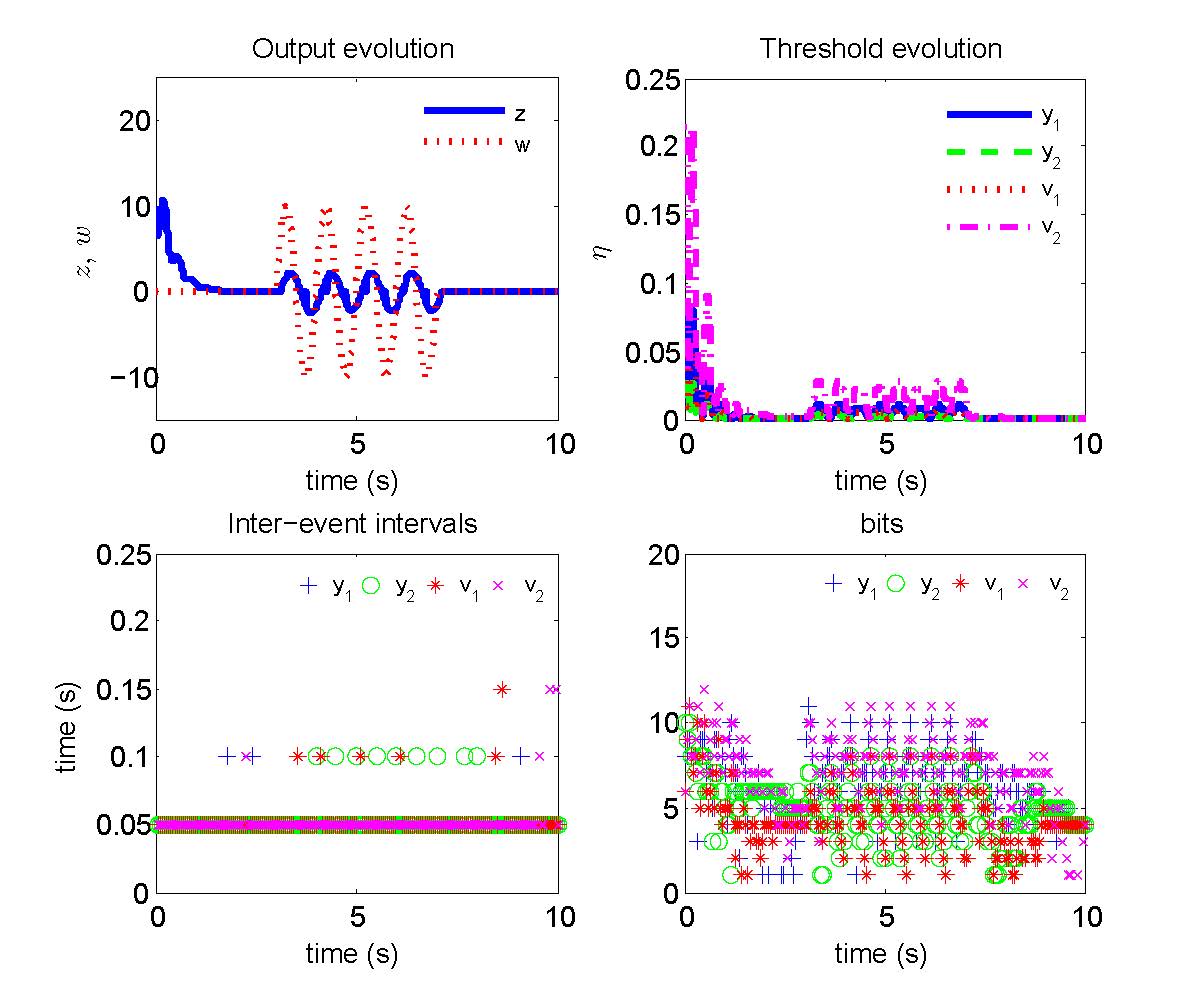 Figure 1