Interpreting the Star Formation Efficiency of Molecular Clouds with Ionising Feedback
Sam Geen, Juan D Soler, Patrick Hennebelle

TL;DR
This study uses advanced simulations to explore how ionising feedback influences star formation efficiencies in molecular clouds, revealing that feedback can explain observed efficiencies and highlighting the complexity of converting observed data to total efficiencies.
Contribution
The paper introduces radiative magnetohydrodynamic simulations incorporating ionising radiation to better understand star formation efficiencies in molecular clouds, aligning simulations with observations.
Findings
Simulated diffuse clouds match observed star-forming clouds.
Ionising radiation reproduces observed SFEs in Milky Way-like clouds.
Observed SFEs are 3 to 10 times larger than total SFEs.
Abstract
We investigate the origin of observed local star formation relations using radiative magnetohydrodynamic simulations with self-consistent star formation and ionising radiation. We compare these clouds to the density distributions of local star-forming clouds and find that the most diffuse simulated clouds match the observed clouds relatively well. We then compute both observationally-motivated and theoretically-motivated star formation efficiencies (SFEs) for these simulated clouds. By including ionising radiation, we can reproduce the observed SFEs in the clouds most similar to nearby Milky Way clouds. For denser clouds, the SFE can approach unity. These observed SFEs are typically 3 to 10 times larger than the "total" SFEs, i.e. the fraction of the initial cloud mass converted to stars. Converting observed to total SFEs is non-trivial. We suggest some techniques for doing so, though…
Click any figure to enlarge with its caption.
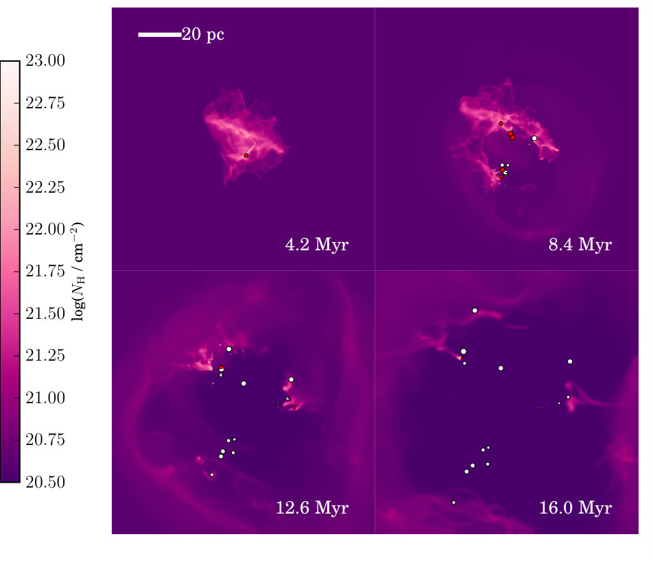 Figure 1
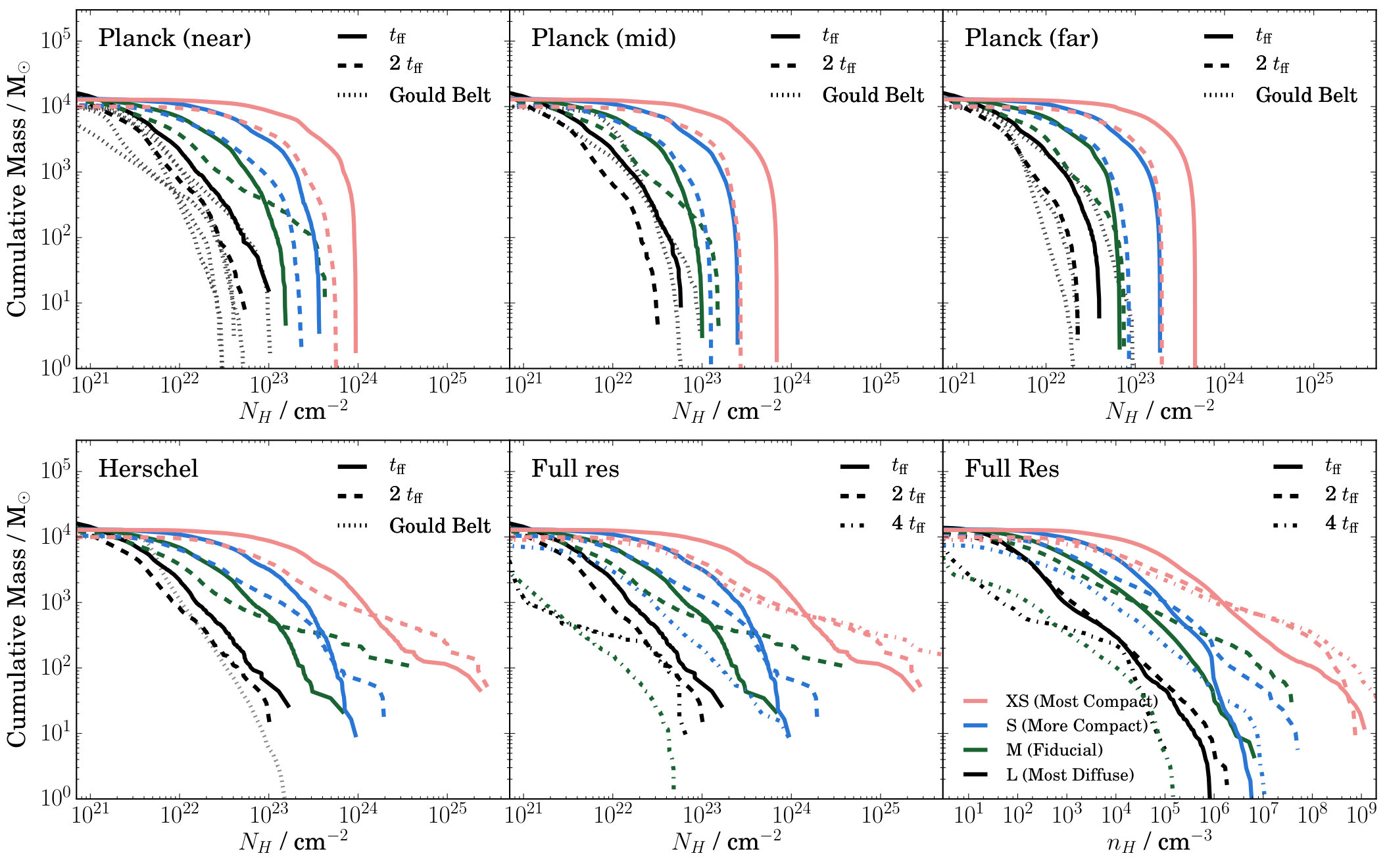 Figure 2
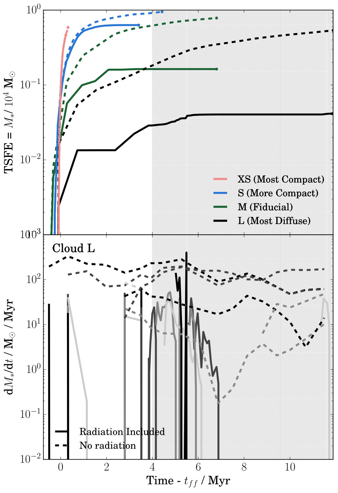 Figure 3
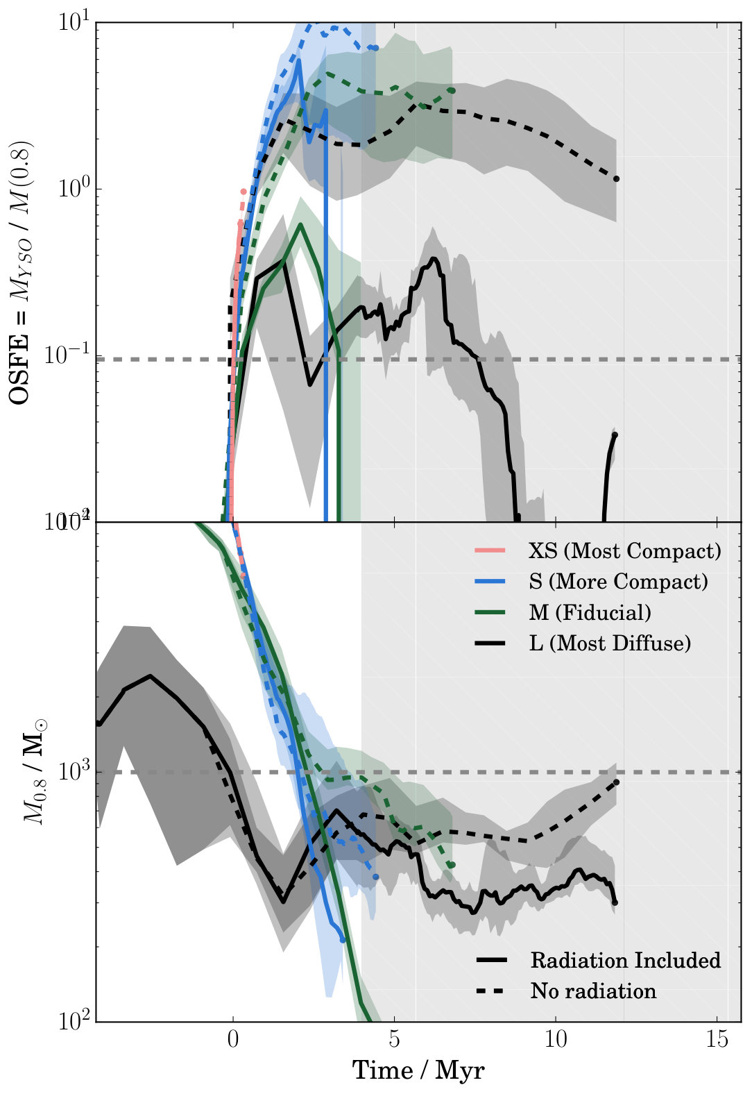 Figure 4
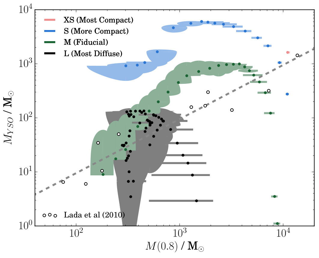 Figure 5
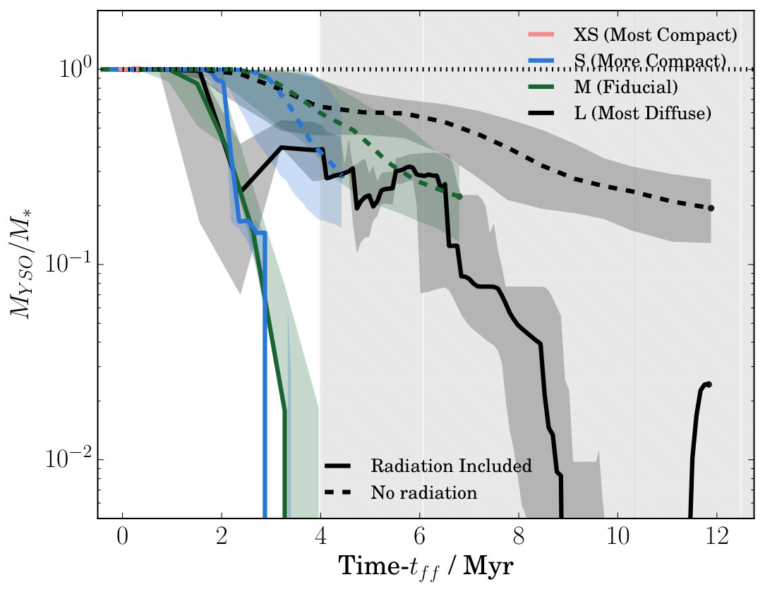 Figure 6
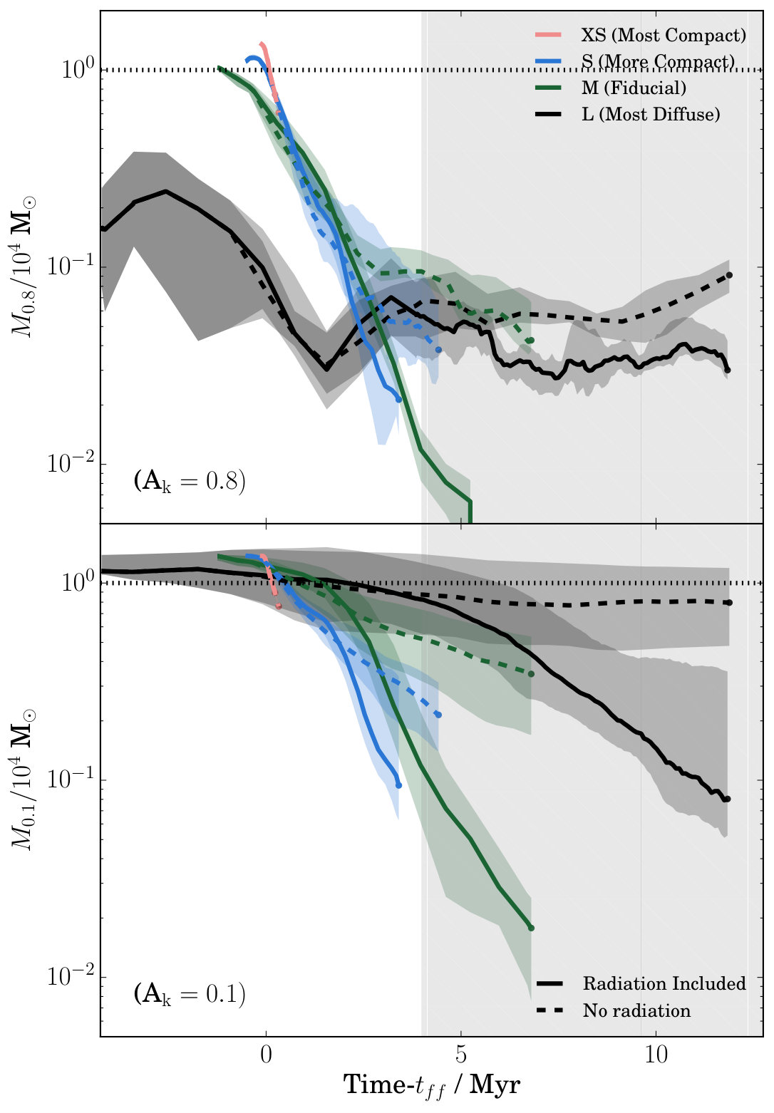 Figure 7
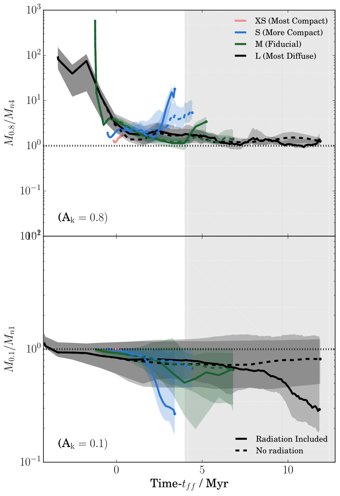 Figure 8
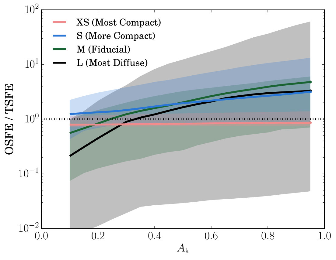 Figure 9
| Cloud Name | / pc a | x / pc b | / Myr c | /cm | / M⊙ / pc2 e | ||
|---|---|---|---|---|---|---|---|
| min | median | max | |||||
| L (Most Diffuse) | 7.65 | 0.03 | 4.22 | 36.0 | 41.8 | 45.1 | |
| M (Fiducial) | 3.40 | 0.026 | 1.25 | 74.5 | 75.6 | 87.0 | |
| S (More Compact) | 1.9 | 0.014 | 0.527 | 160.8 | 175.0 | 185.5 | |
| XS (Most Compact) | 0.85 | 0.0066 | 0.156 | 540.7 | 545.2 | 701.0 |
| Cloud | Distance / pc |
|---|---|
| Near | (150) |
| Taurus | 140 |
| Ophiuchus | 140 |
| Lupus | 140 |
| Chamaeleon-Musca | 160 |
| Corona Australis (CrA) | 170 |
| Mid | (300) |
| Aquila Rift | 260 |
| Perseus | 300 |
| Far | (500) |
| IC 5146 | 400 |
| Cepheus | 440 |
| Orion | 450 |
Peer Reviews
No public reviews on file for this paper yet. If you reviewed it on a platform where reviews are public (OpenReview, ICLR, NeurIPS, ICML), you can paste yours below so the community can read it here.
Videos
No videos yet. Explain this paper in a talk, walkthrough, or lecture? Add one.
\newabbrev\ISM
Interstellar Medium (ISM)[ISM] \newabbrev\CSMCircumstellar Medium (CSM)[CSM] \newabbrev\WNMWarm Neutral Medium (WNM)[WNM] \newabbrev\WIMWarm Ionised Medium (WIM)[WIM] \newabbrev\CNMCold Neutral Medium (CNM)[CNM] \newabbrev\IMFInitial Mass Function (IMF)[IMF] \newabbrev\AMRAdaptive Mesh Refinement (AMR)[AMR] \newabbrev\HGBHorizontal Giant Branch (HGB)[HGB] \newabbrev\SFEStar Formation Efficiency (SFE)[SFE] \newabbrev\TSFETotal Star Formation Efficiency (TSFE)[TSFE] \newabbrev\OSFEObserved Star Formation Efficiency (OSFE)[OSFE] \newabbrev\SFRStar Formation Rate (SFR)[SFR] \newabbrev\YSOsYoung Stellar Objects (YSOs)[YSOs] \newabbrev\YSOYoung Stellar Object (YSO)[YSO] \newabbrev\PDFProbability Distribution Function[PDF] \newabbrev\PSFPoint Spread Function[PSF]
Interpreting the Star Formation Efficiency of Nearby Molecular Clouds with Ionising Radiation
Sam Geen1,3, Juan D. Soler2,3, Patrick Hennebelle3
1 Zentrum für Astronomie der Universität Heidelberg, Institut für Theoretische Astrophysik, Albert-Ueberle-Str. 2, 69120 Heidelberg, Germany
2 Max-Planck-Institute for Astronomy, Königstuhl 17, 69117, Heidelberg, Germany
3 Laboratoire AIM, Paris-Saclay, CEA/IRFU/SAp - CNRS - Université Paris Diderot, 91191, Gif-sur-Yvette Cedex, France Corresponding author: Sam Geen ([email protected])
Abstract
We investigate the origin of observed local star formation relations using radiative magnetohydrodynamic simulations with self-consistent star formation and ionising radiation. We compare these clouds to the density distributions of local star-forming clouds and find that the most diffuse simulated clouds match the observed clouds relatively well. We then compute both observationally-motivated and theoretically-motivated star formation efficiencies (SFEs) for these simulated clouds. By including ionising radiation, we can reproduce the observed SFEs in the clouds most similar to nearby Milky Way clouds. For denser clouds, the SFE can approach unity. These observed SFEs are typically 3 to 10 times larger than the “total” SFEs, i.e. the fraction of the initial cloud mass converted to stars. Converting observed to total SFEs is non-trivial. We suggest some techniques for doing so, though estimate up to a factor of ten error in the conversion.
keywords:
stars: massive, stars: formation Stars, ISM: H ii regions, ISM: clouds Interstellar Medium (ISM), Nebulae, methods: numerical Astronomical instrumentation, methods, and techniques
1 Introduction
In this paper we discuss how star formation relations in local Galactic clouds are set with the use of simulations of isolated star-forming regions. In particular, we measure the response of the simulated clouds to ionising radiation from massive stars, and how this alters the observed Milky Way star formation relations. We also offer some comparison between typical calculations of \SFEin numerical theory and the measurements in observations of nearby clouds.
Stars form in molecular clouds (see review by Hennebelle & Falgarone, 2012). Gas collapses into filaments and cores on the order of a freefall time. In clouds where massive star formation occurs, radiative and mechanical processes drive outflows that resist accretion around the star (see review by Dale, 2015). Over time, these processes disperse cloud material and suppress or halt star formation.
Quantifying star formation efficiencies in nearby molecular clouds has been the subject of much study. In one perspective, it has been proposed that star formation rates are well correlated with gas mass (Lada et al., 2010) or surface density Heiderman et al. (2010) above a certain threshold, and that below this threshold the star formation rate is negligible. In a competing view proposed by Gutermuth et al. (2011), is proportional to . Hony et al. (2015) argue that in practice distinguishing between these two arguments is difficult due to the steepness of the relations and low number statistics. The existence of a threshold for star formation has been discussed by Myers & Benson (1983); Beichman et al. (1986), who use cm*-3*, whereas Onishi et al. (1998); Johnstone et al. (2004) use cm*-2*, equivalent to the limits found by Lada et al. (2010); Heiderman et al. (2010).
There are various discussions as to why there should be a density criterion for star formation. André et al. (2010) argue that the presence of dense filaments is required for dense star-forming cores, which sets a density criterion for core formation. Burkert & Hartmann (2013) argue that the density threshold for star formation is not a single value, but rather represents gas in which self-gravity has begun to dominate. Lee & Hennebelle (2016) characterise the transition from the diffuse cloud to dense protocluster gas as a transition from infalling material to a virialised structure globally supported by a combination of turbulence and rotation.
Krumholz et al. (2012) argue that the star formation rate is in fact correlated to the local free-fall time, which is set by the volumetric density, not the column density. Clark & Glover (2014) analyse simulation results and find no correlation between the column and volume density of gas, the latter of which sets the star formation rate. They do, however, find a link between the observed column density and the effective column density seen by the star. The link between observed star formation relations and the theory of star formation on small scales is still an open question.
The picture of star formation is complicated by the introduction of feedback cycles driven by energetic stellar events. In particular, a great deal of attention has been given to the role of ionising feedback. Numerical simulations by Dale et al. (2005); Gritschneder et al. (2009); Peters et al. (2010); Walch et al. (2012); Dale et al. (2012); Colin et al. (2013); Howard et al. (2016) confirm that ionising UV photons are able to drive outflows in molecular clouds that disperse the supply of dense gas during star formation events. Authors such as Whitworth (1979); Matzner (2002); Krumholz et al. (2006); Goldbaum et al. (2011); Kim et al. (2016) have constructed (semi-)analytic models including radiation feedback to study star formation efficiencies in clouds. One such model by Matzner (2002) find that % of the mass in clouds is converted to stars before ionising radiation disperses the cloud.
In our previous work (Geen et al., 2015, 2016), we focussed on the link between simulations and analytic theory. Despite the complexity of the environments, we were successful in reproducing the quantitative behaviour of simple simulated HII regions with analytic theory (Spitzer, 1978; Dyson & Williams, 1997; Hosokawa & Inutsuka, 2006; Raga et al., 2012; Tremblin et al., 2014). We were also able to explain the evaporation of dense clumps in our simulations using the models of Bertoldi & McKee (1990). By comparison, in this work we wish to link our simulations to observed clouds. We compare both the gas structure in observed clouds and the star formation efficiencies. The former is important because our initial conditions are highly idealised, and we cannot be certain how relevant our simulation results are to observed star-forming clouds otherwise.
The goal of this paper is to compare the results of observational studies of local clouds with projections of simulated star forming regions. In particular we wish to understand how ionising radiation sets star formation relations in simulations, and provide insight into how observed star formation efficiencies are obtained. We focus on the relation of Lada et al. (2010), who measure total \YSOnumbers and gas masses. By comparison, Heiderman et al. (2010) use surface densities, which we cannot reproduce accurately with our limited \YSOmass resolution.
We stress that this comparison is for local Milky Way clouds, where fully resolved gas structures and stellar populations are available. Koepferl et al. (2016a); Koepferl et al. (2016b); Koepferl et al. (2016c) give detailed techniques for calculating star formation rates and efficiencies for cases where the cloud is not resolved and reliance on tracers is necessary, such as in extragalactic studies (e.g. Gao & Solomon, 2004).
In this paper we are able to discuss the role of ionising radiation in producing these observed star formation relations, and compare them to typical \SFEmeasurements in theoretical work. The closest previous study looking at this problem, Clark & Glover (2014), omitted energetic stellar feedback processes and thus ended its analysis at a \SFEof 10%. We purposefully use a model for the emission rates of photons that does not depend on the stochasticity of the \IMFin clusters below masses of , in order to make our results simpler and easier to interpret. Similar studies of ionising radiation in clouds with varying initial properties have been performed by, e.g., Peters et al. (2010); Dale et al. (2012); Howard et al. (2016), although using different methods and initial conditions, and without close comparison Milky Way clouds. Although the focus of this work is in using simulations to interpret observed clouds, we discuss the theoretical implications at the end of the paper.
In Section 2 we introduce the simulations used in this study. In Section 4 we discuss our results. We begin by discussing the post-processing techniques used to approximate observations of our simulated clouds. We then present the total star formation efficiency of the clouds over their lifetime. We extend this to an estimate for the observed star formation efficiency of these clouds. We analyse the density distribution of these clouds in comparison to local clouds, and estimate the likelihood of observing each cloud at each point over its lifetime. We then discuss the implications of our study, and some of the limitations of our techniques.
2 Numerical Simulations
In this section we review the simulations used in this paper. We simulate a set of isolated turbulent molecular clouds with sink particles representing clusters of stars. These particles emit ionising photons that heat the gas they encounter. We use the radiative magnetohydrodynamic Eulerian \AMRcode RAMSES (Teyssier, 2002; Fromang et al., 2006; Rosdahl et al., 2013).
2.1 Initial Conditions
We run simulations of four clouds with varying mean density, each with initial gas mass . These clouds are labelled “L”,“M”,“S” and “XS”, in increasing order of initial compactness. We summarise these initial conditions in Table 1. The last three clouds have identical initial conditions to the Fiducial, More Compact and Most Compact clouds in Geen et al. (2015). Cloud L is included in this work to increase the range of the study. The clouds have an initially spherically symmetric structure, with an isothermal profile out to and a uniform sphere of radius outside that with 0.1 times the density just inside . The total box length in each dimension is 48 times in each simulation. We apply an initial velocity field with a Kolmogorov power spectrum () with random phases such that the cloud is in approximately virial equilibrium.
2.2 Numerical Setup and Sink Formation
Each simulation has a root grid of cells. We fully refine a sphere of diameter half the box length, encompassing the initial cloud, for two further levels. Gas that exceeds the Jeans criterion by a factor of 10 anywhere in the simulation volume is allowed to refine up to a total of 4 additional levels above the base grid (5 levels in the L cloud). We “relax” each cloud by halving the gravitational forces for one freefall time in order to allow the density and velocity fields to couple.
The sink formation recipe we use is described in detail in Bleuler et al. (2014); Bleuler & Teyssier (2014). We identify clumps above a threshold given by 10% of the Jeans mass in cells at the highest refinement level. If a clump exceeds ten times this threshold, we form a sink particle. Each sink particle accretes 90% of the mass above the sink formation density threshold at each timestep.
2.3 Radiative Transfer and Cooling
We track the advection of ionising photons on the AMR grid using a first-order moment method described in (Rosdahl et al., 2013). We allow the ionising photons to interact with the neutral gas, and track the ionisation states of hydrogen and helium.
We implement the cooling function described in Geen et al. (2016). The cooling in neutral gas is based on Audit & Hennebelle (2005), which includes a background heating term and a fit to Sutherland & Dopita (1993) above K. Cooling of photoionised gas is treated as in Rosdahl et al. (2013), with a piecewise fit to Ferland (2003) to describe cooling on photoionised metals.
2.4 UV Source Properties
Each set of initial conditions is run twice, once with no ionising UV photons (labelled “NRT”), and once where ionising UV photons are emitted from sink particles (labelled “RT”). Our resolution is not sufficient to resolve individual stars. Rather, in simulations labelled “RT”, we impose a total hydrogen-ionising photon emission rate of , where is the total mass in sink particles. This is calculated by Monte Carlo sampling a well-sampled stellar population using a Chabrier IMF (Chabrier, 2003), with hydrogen-ionising emission rates for each star from Vacca et al. (1996); Sternberg et al. (2003) (see Appendix A in Geen et al., 2016, for further details).
We distribute this total photon emission rate across the sink particles with a weighting , where is the mass of a given sink particle and is a fit to the photon emission rate for a range of stellar masses given in Vacca et al. (1996); Sternberg et al. (2003). is a scaling factor that we set to 0.3 as a heuristic to weight emission towards more massive clumps. We adopt this model, rather than sampling stars using a Monte-Carlo scheme, to avoid stochasticity in the emission rate sampled since this would require a larger sample of simulated clouds to reach convergence.
3 Observations
We use a number of observational results for which we are able to find reliable analogues in our simulation results. The most important points of comparison in this work are the \YSOcount and gas masses for Gould Belt clouds given in Lada et al. (2010). As stated in Section 1, this is not the only observational study to tackle this problem. However, since these authors use masses and not surface densities, and since we do not produce individual stars in our simulations, this paper provides a good point of comparison. In addition, these measures are relatively robust to systematic errors in converting the observations to physical quantities, making them ideal points of comparison with simulation results.
In addition to the previously mentioned results, we use two sets of column density maps of the same objects, one from Planck and one from Herschel, to compare cloud structures to our simulation results on a pixel-by-pixel basis. For completeness, we summarise how each of these measurements are obtained, and how reliably they can be compared to our results.
3.1 YSO Counts
Lada et al. (2010) use a \YSOcount in each of the Gould Belt clouds to produce \SFRestimates. To find , they use infrared surveys from a number of sources (see the paper for a full list). Most of the clouds have been observed with the Spitzer Space Telescope, and are expected to be virtually complete111Based on tests performed using our simulations, only the densest cloud simulated in this paper has sufficient extinction to make stars in the cloud completely undetectable.. The authors estimate that the least well sampled clouds have an error in of no more than a factor of 2. In these clouds they estimate the stellar ages to be Myr (see Covey et al. (2010). They use a median stellar mass of 0.5 to convert to a mass for \SFRestimates.
In this paper, we assume a maximum \YSOage of Myr, which is approximately the lifetime of the most massive stars. Beyond this, the \YSOcounts will begin to be incomplete. We use a larger \YSOage than Lada et al. (2010) since our clouds are evolved for a longer time than the given age of the observed stellar populations. The 1 Myr error is reflected in the errors in each of the figures. In addition, we shade our figures 4 Myr after in each cloud. This is the point at which \YSOcounts will start to become noticeably incomplete, and supernovae start to occur. We do not include supernovae in this paper for reasons of simplicity, and to avoid stochasticity in choices of stellar masses. Thus, any results in this region become more speculative, assuming that supernovae do indeed strongly affect the properties of the cloud.
3.2 Gas Masses
Lada et al. (2010) produce column density maps from extinction maps using the NICER technique (Lombardi & Alves, 2001). This technique measures the extinction of background stars by intervening material. Since the only parameter that affects extinction measurement is the amount of mass between the observer and the background star, it converts robustly to a column density. The authors then sum the masses of each pixel above a given extinction threshold to find a gas mass for the cloud. We define this to be for an extinction . Lada et al. (2010) focus on and , which are roughly analogous to all the mass in the cloud and the mass in only the densest regions, respectively.
For each of our simulation outputs, we produce hydrogen column density () maps along the three cartesian axes of the simulation volume. This is just the total mass along a line of pixels, divided by the area of one pixel, converted to hydrogen number using a mass fraction . We convert to extinction (in mag) using the relation cm*-2* mag*-1*, as given in Lombardi (2008). These maps for simulation L-RT are shown at intervals of in the cloud in Figure 1.
As in Lada et al. (2010), we focus on masses contained within pixels above an extinction of and . These errors are illustrative, and provide estimates for how the gas masses we produce should vary if the extinction thresholds are changed.
3.3 Planck Column Density Maps
We use total gas column density derived from the dust optical depth estimated from the Planck observations toward nearby (d ¡ 500 pc) molecular clouds. Nominally, we use maps of each of the Gould Belt objects listed in Planck Collaboration XXXV (2015) (see Table 2). For each object we use the dust optical depth at 353 GHz () as a proxy for the total gas column density (). The map is derived from the all-sky Planck intensity observations at 353, 545, and 857 GHz, and the IRAS observations at 100m (3000 GHz), through a modified black body spectrum fit, which also yielded maps of the dust temperature and of the dust opacity spectral index (Planck Collaboration XI, 2014). These parameter maps were estimated at 5’ resolution.
To scale from to , following Planck Collaboration XI (2014), we adopted the dust opacity,
[TABLE]
Variations in dust opacity are present even in the diffuse ISM and the opacity decreases systematically by a factor of 2 from the denser to the diffuse ISM (Planck Collaboration XXIV, 2011; Martin et al., 2012; Planck Collaboration XI, 2014), but our results do not depend on this calibration.
The maps of the individual regions are projected and resampled onto a Cartesian grid with the gnomonic projection procedure described in Paradis et al. (2012). The present analysis is performed on these projected maps. The selected regions are small enough, and are located at sufficiently low Galactic latitudes that this projection does not impact significantly on our study.
3.4 Herschel Column Density Maps
In order to test our models of column density distributions with observations at higher angular resolutions than those possible with Planck, we use the gas column density map derived from the Herschel observations towards the Serpens South region of the Aquila Rift molecular cloud (d=260 pc, Prato et al., 2008).
We use the 36”5 resolution NH2 column density map derived from a modified black body spectrum fit to the 70-, 160-, 250- , 350-, and 500-µm Herschel observations, described in Konyves et al. (2015) and publicly available in the archive of the Herschel Gould Belt Survey2 222http://www.herschel.fr/cea/gouldbelt (HGBS, André et al., 2010) project. The instrument’s resolution is below our spatial resolution at the distance of the Aquila cloud.
4 Results
In this section we present the results of our comparisons with the observational quantities listed above. The purpose of this section is to use the simulations to describe how these observations can be physically interpreted, and how well typical simulation \SFEmeasurements can be compared to observed \SFEmeasurements.
The broad picture of star formation in molecular clouds is well established. Stars form from dense cores in molecular clouds. The most massive of these stars inject energy into the surrounding gas in various forms, and will, depending on the properties of the cloud and stars, end star formation in the cloud and inject energy, mass and radiation in the surrounding medium.
In our simulations, ensembles of stars are represented as sink particles. Sink particles emit radiation corresponding to the emission rate of a typical \IMF(see Section 2). This radiation heats the gas to K, causing the surrounding material to expand and push away infalling matter. This prevents further accretion onto this sink, as well as nearby sinks. Eventually the entire cloud is dispersed, halting star formation globally in the cloud.
There are a number of separate star-forming volumes in our cloud, represented by clusters of sink particles. In panel 2 of Figure 1 at 8.4 Myr, these volumes are found on the edge of the central ionisation front. This might imply that star formation is triggered by the presence of an ionisation front. However, since our star formation efficiency is reduced by the presence of star formation, we invoke the suggestion of Dale et al. (2015) that these locations would form stars anyway in the absence of an ionisation front. We note that there is no “central” source for the ionising radiation in panel 2. Rather, the sources of ionising radiation follow the expanding shell via gravitational attraction, and the star cluster becomes unbound by 16 Myr.
4.1 Comparisons with Observed Cloud Structure
In Figure 2 we compare the density distribution of material in our clouds against that of the nearby Gould Belt clouds, listed in Table 2, using the Planck and Herschel maps. We plot the cumulative mass in bins of descending density for our simulations at and as well as the clouds described in Section 3. We convolve our results with a \PSFcorresponding to the instrument FWHM of 10’ at three distance bins. These are Near at 150 pc, Mid-range at 300 pc and Far at 500 pc. This removes signal from higher column densities. In the Herschel comparison, we use the Aquila cloud, which is at a distance of 260 pc. The instrument FWHM is 0.2’, giving a \PSFof size 0.06 pc at this distance. This is smaller than the maximum spatial resolution in our simulations. The convolved density distributions are thus not significantly different from those taken at full resolution. The most diffuse cloud, L, matches the Planck and Herschel results most closely, although cloud M also matches some of the observed clouds at 2 .
When the results are taken at full resolution, we are able to detect denser material. Most of the clouds become denser at later times as mass accretes onto dense clumps. These densities can exceed the sink formation threshold since not all of the densest gas is accreted in a single timestep, and the freefall times at these densities are short. This pattern occurs for both column density and volume density . The only cloud where this is not the case is the run L-RT. Here, HII regions driven by ionising radiation from the sinks creates cavities in the cloud at (see Figure 1), reducing the number of pixels with high column densities.
Higher densities are reached in the more compact initial conditions. As well as the initial conditions being denser by construction, the maximum spatial resolution is higher due to the smaller box size. Note that clouds L and M have comparable spatial resolutions. Clouds with the density structure of clouds S and XS are not found in observed local star-forming regions (see Figure 2). In addition, these clouds already have a large quantity of gas above ( cm*-2*) at , requiring some mechanism to rapidly collect this much gas without forming stars. We posit that extreme environments are needed to create such objects, if indeed it is possible to collect this much dense gas without forming stars.
4.2 Total Star Formation Efficiency
The first quantity we use to measure \SFEis one traditionally used in in theoretical work (e.g. Dale et al., 2012; Colin et al., 2013; Federrath, 2015; Howard et al., 2016). This is the total fraction of the initial cloud mass accreted onto sink particles, which we call the \TSFE. in this work is set to . We plot this quantity in Figure 3.
In the simulations without radiation, the \TSFEtends towards 1 over several for the cloud as a whole (see Table 1). With radiation, the stellar mass reaches a plateau after 1-2 . This plateau corresponds to the time at which the majority of dense gas is dispersed. In the XS simulation, this plateau is never reached due to the density of the cloud preventing ionised outflows (see Geen et al., 2015). In clouds L and M, a number of small plateaus are reached before star formation continues. This corresponds to separate star formation events within the cloud that are ended locally by ionising radiation.
In the NRT simulations, the sink particles accrete continuously over the course of the simulation until the supply of gas is exhausted. In the RT simulations, each sink particle typically accretes during a single burst anywhere between a few hundred kyr to a few Myr. After this time, radiation decouples the sink particle from the dense gas and accretion ends. The mass-weighted mean accretion time is 0.93 Myr in M-RT and 0.47 Myr in L-RT. The median accretion time is 0.63 Myr in M-RT and 0.30 Myr in L-RT. 7 of the 16 sinks in L-RT accrete for less time than the time resolution of our simulation outputs, so this figure is moderately biased towards shorter values. Feedback does not significantly shorten the accretion times in S-RT and XS-RT.
The SFE is roughly 10 times lower when ionising radiation is included than without in the L cloud, 3 times in the M cloud and closer to unity in S and XS. The XS simulations were not completed due to the short timestep in these simulations and their relative cost.
In Figure 9 of Dale et al. (2012), clouds with mass and radius above 10 pc do not form stars, while below 3 pc, ionising radiation is ineffective at altering the dynamics of the cloud. Our results are largely in agreement (see Table 1 for initial radii ). Clouds L and M both have above 3 pc, and have reduced SFEs. Cloud L in particular is completely unbound by ionising radiation. Cloud S has an initial radius of 1.9 pc and has some reduction in response to ionising radiation, while Cloud XS () does not respond to ionising radiation at all. Note that since we allow the cloud to relax with half gravity for one freefall time, these initial radii are underestimates of the effective cloud radius at the time stars begin to form.
4.3 Reproducing Observed Star Formation Efficiency
In this section we attempt to reproduce observed star formation efficiencies from local clouds, where \YSOcounts and gas columns are well resolved. We call this \OSFE, which is given by (see Section 3). This quantity is analagous to in Lada et al. (2010), where . The authors in this paper produce additionally star formation rates per star formation timescale and per freefall time, derived using . However, since these are quantities with their own uncertainties, we focus on itself.
In Figure 4 we plot the \OSFEas a function of dense gas mass over time for each of the simulations. \OSFEis defined as / . is the mass in sinks accreted over the last , which we choose to be 3 Myr (consistent with Covey et al., 2010; Lada et al., 2010, noting that these authors measure the median and not the maximum \YSOage). As in Lada et al. (2010), we include only sink particles inside contours of when calculating . Note that Lada et al. (2010) measure the number of \YSOs, , not the mass. They convert these using a median \YSOmass 0.5 , i.e. {\rm M}_{\mathrm{\mathord{\odot}}}$$N_{\mathrm{YSO}}. is the total mass in all the pixels in the gas column density maps where . We allow to vary by 0.1 and to vary by 1 Myr, and calculate each quantity for the line of sight along each Cartesian axis. We plot the median value as a solid or dashed line, and the maximum and minimum values as a filled area with the same colour as the line.
We overplot a line at \OSFE=10%, corresponding to the fit to local clouds given in Figure 4 of Lada et al. (2010). Without ionising radiation, the \OSFElies well above this line. The denser clouds have higher star formation efficiencies, although the variation is of the same order as the estimated errors (the shaded areas in Figure 4). With ionising radiation, the \OSFEis reduced similarly to the fraction of reduction in the \TSFE. In other words, the \OSFEis reduced by a factor of 10 in L, 3 in M and just over unity in S. There is, however, more variation due to the age of the \YSOsand the variations in dense gas mass.
All of the initial conditions for the clouds contain some gas above , with the three densest clouds having nearly all of their mass above this threshold. Given this, the gas is rapidly converted into stars. In the denser clouds, where the freefall time is very short, ionising radiation is unable to drive outflows within a short enough time to prevent most of the cloud from being accreted onto sinks. Only the L cloud reaches a quasi-equilibrium state in which the quantity of dense gas plateaus at around .
4.4 Likelihood of Observing a Given SFE
In Figure 5 we plot the YSO mass against the mass of gas above , , for each of the simulations with ionising radiation included. We interpolate the values of each quantity to intervals of 0.2 Myr in order to obtain the probability of observing the cloud in a given state. We overplot the same fit to Lada et al. (2010), = 0.1 , given in Section 4.3.
All of the clouds start at high and low . They rapidly reach a peak , before tailing off to low values of and as the supply of dense gas is depleted (see Figure 4). In cloud L, in the late phase of the cloud’s evolution, drops rapidly while remains constant. This suggests that it is possible to accumulate supply of dense gas that is relatively quiescent in clouds that have been recently star-forming. Looking at the lower right panel of Figure 2, the maximum gas volume density at 4 is below the threshold for forming stars in clouds L and M, despite the presence of gas above cm*-2*. Since \YSOshave a maximum age ( Myr) longer than the typical accretion time onto a protocluster (0.1 to 1 Myr), the presence of a \YSOis not a guarantee that stars are still actively forming in a particular volume.
Our L cloud, which most closely represents the Gould Belt clouds’ density distribution (see Section 4.1), matches the fit of Lada et al. (2010) to within the estimated spread in and . The initial phase of star formation is rapid, and so is less likely to be observed than the main sequence of the evolution. Finally, the late phase of cloud dispersal and minimal star formation is not sampled by the Gould Belt objects owing to their ages. The low number of nearby clouds and the limited sample of simulated clouds in this study prevents a more statistical comparison.
In addition to being less similar to local clouds, the denser clouds in our simulations live for shorter times. The most compact, XS, is only sampled for one point on our curve, by chance on the Lada et al. (2010) fit. Even if these clouds are formed in equal numbers with more diffuse clouds, we expect them to be detected in fewer numbers due to their shorter lifespans.
5 Mapping Observed to Total Star Formation Efficiency
In this section we discuss how well typical simluated quantities can be mapped to local observations. For the sake of clarity, we first compare stellar masses and gas masses independently.
5.1 YSO vs Total Stellar Mass
In Figure 6, we compare the mass in recently formed stars with the total mass in stars formed over the lifetime of the cloud. Up to 2 Myr, the lower end of our \YSOage measurement, the ratio is unity. After this time, we begin to exceed the maximum age of the most massive stars in the cluster, and the ratio drops. The results of Lada et al. (2010) are most relevant in this early stage, assuming that their \YSOcount is complete and no earlier phase of star formation occured. The age of stars, and loss of older stars to \YSOcounts, is particularly important in the L cloud, which is most similar to the nearby Gould Belt clouds (see Section 4.1), due to the long freefall times in the cloud.
5.2 Evolution of Dense and Diffuse Gas Mass
The relation between gas mass above a certain extinction threshold and the total initial gas mass of the cloud is more complex. Since we use a constant , the behaviour of is identical to the discussion in Section 4.3. Initially, (chosen to capture all of the material above the background density) is similar to . It starts above due to capturing part of the background in the column. Over time, the ratio drops as gas is converted to stars. It drops faster when ionising radiation is included, since this heats and disperses a proportion of the cloud mass.
Up to 4 Myr in the L cloud, , since the conversion of gas to stars is inefficient. We thus expect \TSFEto be very similar to in this cloud, but only at early times. In denser clouds and later times, we expect \TSFEto map badly to \OSFE.
5.3 Column vs Volume Density Thresholds
Various authors have discussed whether the mass in dense gas measured using column density thresholds on 2D maps has any relation to the mass above a volume density threshold. We refer to column thresholded masses as as before. Volume density thresholded masses are given as , where is given by log( / cm*-3*), where the volume density threshold is . This comparison has already been made in a similar study by Clark & Glover (2014), albeit without radiation. These authors find a poor match between the two quantities, with being much larger than .
In the upper panel of Figure 8, we plot the ratio (see also Clark & Glover, 2014). In the lower panel we plot . The latter thresholds attempt to capture all material above the background density. After , both ratios are close to unity, until ionising radiation begins to disperse the gas. In this case, drops faster than because the former is more affected by the radiation, which disperses the gas with the highest volume density, where sink particles form, first. Conversely, drops after radiation begins to disperse the gas. This is because background material is swept into diffuse shells, which increases while removing gas from the cloud, which reduces .
While there is not a single 1:1 mapping between masses derived from 2D column density maps and masses above a volume density threshold, we find that for conditions similar to local star-forming clouds, for the majority of the lifetime of the L cloud, and for a fraction of the lifetimes of the denser clouds. This mapping is reasonable for local clouds, which are similar in density structure to our L cloud, but as the denser clouds and the results of Clark & Glover (2014) show, there is not a single mapping between the two quantities for all possible clouds.
5.4 Role of Extinction Threshold
We now investigate the effect that the choice of extinction threshold has in setting the \SFE. In Figure 9, we plot the ratio OSFE() / TSFE against . There is a large degree of variation in the results at each value of due to variation with time. The results for XS-RT are roughly constant since nearly all of the gas is above ( cm*-2*, see Figure 2). The median values for the other simulations follow a roughly similar trend above . This suggests that any value of above this limit can be used to produce a convergent star formation efficiency.
We find a systematic trend to higher values of OSFE()/TSFE for increasing , since as the threshold increases less gas is contained within it. Since is typically smaller than (see Figure 4), the ratio OSFE()/TSFE can be over 1 for larger values of .
All of the simulations display at least a factor of ten variation in OSFE/TSFE over time for a given value of . This makes an exact conversion from OSFE to TSFE difficult. Some time variation can be accounted for by studying the time evolution of the stellar populations and HII regions (see, e.g., Tremblin et al., 2014). Older clusters exhibit a smaller OSFE/TSFE, since the number of YSOs is truncated at 3 Myr, while the TSFE includes all stars formed by the cloud.
6 Discussion
In this section we discuss the results and implications of this work. We provide points of comparison to other authors, and suggest cases where further work is needed to expand on the conclusions of this paper.
6.1 Relative Importance of Feedback Processes
Producing a model for the self-regulation of star formation in clouds that accurately describes all the important processes is an extremely challenging task and one that is beyond the scope of this paper. However, it is clear that energetic stellar processes that reverse gas infall around protoclusters are an important dynamical process in setting the star formation efficiencies of molecuar clouds, regardless of the details of how such processes behave and interact with the cloud.
A number of aspects of the problem were omitted from this project that would have increased the complexity and cost of the study. Our numerical resolution does not allow us to treat each sink as an individual star. This has two effects. Firstly, we do not resolve the full N-body behaviour of a young star cluster. Secondly, we adopt a simple prescription for the number of photons per stellar mass in the cluster. The advantage of this is that it avoids the stochasticity of small clusters with a poorly-sampled \IMFthat would require an extensive parameter study of the range of possible stellar masses and photon emission rates. This undersampling of the IMF is likely to disappear for clusters above (see Appendix A of Geen et al., 2016).
We also neglect processes such as stellar winds, protostellar outflows, radiation pressure and supernovae. More sophisticated models and higher resolution are needed to increase the physical fidelity of our results and allow closer comparison to observations. This is not a trivial problem, particularly if we wish to build a quantitative, descriptive model for how these processes behave. Recent 1D analytic calculations of wind and radiation pressure-dominated HII regions by Rahner et al. (2017) suggest that different processes dominate at different times and in different environments. There exists a point for which winds and radiation pressure dominate over photoionisation in HII regions. For analytic discussions of the interaction between winds and ionising radiation in HII regions, see Weaver et al. (1977); Capriotti & Kozminski (2001).
Numerical simulations of Rey-Raposo et al. (2017) suggest that stellar winds do indeed reduce the star formation rates of clouds, while supernovae, which occur later, have less of an effect. Dale et al. (2014) finds less dynamical effect from winds when ionising radiation also included. The disagreement between various authors as to the importance of winds remains an outstanding problem.
6.2 Cloud Structure and Environment
Molecular clouds are turbulent structures collapsing under gravity. Krumholz & Tan (2007) state the importance of turbulence in lowering star formation efficiencies. In our initial conditions, we add a turbulent velocity field, but this decays over time in the absence of external sources of turbulence.
We do not address directly in this work the origin of molecular clouds or any environmental effects that influence molecular cloud formation and destruction. Instead, we invoke starless clouds of a certain density ab initio.
The issue of whether or not an isolated sphere is an appropriate model for a molecular cloud has been addressed by Rey-Raposo et al. (2014), who compare clouds taken from a galactic context with isolated spheres. They find that the galactic environment is important in setting the velocity structure of the cloud. In addition, Dobbs & Pringle (2013) find that cloud mass evolution is strongly affected by the passage of the cloud across spiral arms.
Ibáñez-Mejía et al. (2017) use simulations of a kiloparsec-scale box and follow the collapse of clouds under the influence of supernovae and gravity. They argue that supernova driving is a secondary effect on the dynamics of the cloud, and that gravitational energy from cloud collapse, as in our isolated simulations, remains the principal driver of kinetic flows in the cloud.
In our work, nearly all of the mass in the denser clouds (M, S and XS) is in gas identified in the dense phase (above or cm*-2*). This means that stars are able to form rapidly before ionising radiation is able to disperse the host cloud. These artificial initial conditions cannot be linked directly to a formation mechanism, and the presence of dense gas ab initio should be treated with caution.
Parameter studies such as this work are easier to perform in isolated spheres, since the properties of the spheres can be carefully constrained. In addition, zooming onto individual clouds presents a numerical challenge. Nonetheless, the issue of galactic environment in changing the structure and dynamics of the cloud through tidal fields, mass accretion and external feedback processes should be carefully considered.
6.3 Density Thresholds for Star Formation
The existence of a density threshold for star formation is an ongoing subject of debate. In particular, the relationship between mass above a given column density and mass above a given volume density is not clear. Krumholz et al. (2012), for example, claim that by using a volume density threshold, a universal star formation relation can be found, and that the column density threshold is a reflection of this relation.
In our paper, we find that during most of the lifetime of the cloud, there is a rough proportionality between gas mass above a column density threshold and gas mass above a volume density threshold for all of our clouds, with or without ionising radiation. However, Clark & Glover (2014) find a larger range of conversion factors, suggesting that this is a chance occurrence. However, a wider parameter study is needed to confirm this.
A key argument of Lada et al. (2010) is that star formation rates are linked to the mass in dense columns of gas, as opposed to the total mass of a cloud. Clark & Glover (2014) suggest that there is a link between the surface density that the star “sees” and the projected column density to the observer. Another possibility they suggest is that denser columns are less likely to be polluted by background material. In addition to this, we find that the apparent total mass of the cloud is particularly sensitive to HII regions, which disperse material into relatively diffuse and mostly non-star-forming shells. There also does not appear to be one single density threshold that causes star formation efficiencies to converge to a single value. We find some convergence above , albeit with a large error.
We do not explore the arguments of Heiderman et al. (2010) or Gutermuth et al. (2011) based on surface density, owing to the limited mass resolution of our cluster’s sink (i.e. star) particles. Hony et al. (2015) argues that it is not possible to distinguish between models that assume a flat dependence between dense gas and stellar mass, and models that assume a power law dependence on gas density. The issue is complicated by the fact that these relations only become apparent over a number of star-forming volumes (Kruijssen & Longmore, 2014), and break down on small scales due to incomplete sampling.
Parmentier (2017) argues that the existence of a linear relationship between dense gas mass and star formation rate requires a particular cloud structure, otherwise the relationship becomes super-linear. This is because the dense central clumps are fed slowly by infalling material, rather than collapsing quickly over one freefall time, which Krumholz & Tan (2007) discount. The dynamical evolution of the cluster is also likely to confuse results in older clusters.
6.4 Interpreting Star Formation Efficiencies
In this work we have measured the \SFEin a set of turbulent molecular clouds of varying initial density. We do this in two ways. The first, which we call TSFE, is typically performed on numerical simulation results. Here, we take the total fraction of the initial cloud mass converted into stars. In the second, which we call OSFE, we reproduce the measurements of Lada et al. (2010), taken from observations of resolved, nearby clouds, which is defined as the ratio of mass in \YSOsto the mass in gas above a column of dense gas. There is not a single, clean conversion between these two measurements. Thankfully, both measurements are simple to perform on numerical simulations.
For extragalactic clouds, where stellar populations are not resolved and the use of molecular tracers is necessary, the problem becomes more complex. Koepferl et al. (2016a); Koepferl et al. (2016b); Koepferl et al. (2016c) describe various techniques that can be used to produce accurate estimates of extragalactic star formation efficiencies. This is an important aspect, since it enables us to expand simulation results beyond local conditions and broaden comparisons with star formation across cosmic time. If indeed the structure of local clouds is similar enough that the convergent \SFEis a result of initial conditions rather than a universal star formation relation, this should be more carefully explored.
Our results agree broadly with those of Dale et al. (2012), who use different numerical techniques to this work but model the same physical processes. However, we do not perform a rigorous cloud-by-cloud comparison to determine how precise this agreement is. Similarly, a link between numerical theory and simple analytic models such as those by, e.g., Matzner (2002), should be more carefully established.
Our results also agree qualitatively with those of Colin et al. (2013). Star formation occurs in local bursts, where individual clouds are dispersed by HII regions rather than maintaining an equilibrium of star formation. The OSFE is likely to enhance the appearance of an equilibrium state, since it uses \YSOswith a minimum lifetime of a few Myr, which smooths over much shorter bursts of active star formation. Colin et al. (2013) also argue that local variations of compactness can cause locally increased star formation rates.
Howard et al. (2016) studies a similar problem. Curiously, they find that ionising radiation has only a limited effect on the star formation rate of the cloud. They instead argue that gravitational boundness is more important. However, their simulations do not reach the point of gas exhaustion in the cloud, suggesting that ionising radiation is less initially significant than at late times, when the cloud has been overtaken by HII regions.
As discussed previously, the interaction between different forms of feedback in setting the \SFEis highly complicated. A convergence between numerical simulations, observational measurements and analytic theory is needed to fully grasp the problem both descriptively and quantitatively.
7 Conclusions
We use radiative magnetohydrodynamic simulations with self-consistent star formation and ionising radiation from massive stars to explore the origins of observed local star formation relations. Energetic processes from massive stars drive outflows in the gas around them and end star formation in the volume around them.
We simulate a series of isolated clouds of various initial densities with and without ionising radiation. We compare the cumulative density probability distribution function (PDF) of these clouds to local clouds in the Milky Way by convolving our column density maps with the appropriate point spread function (PSF). We find that the more diffuse clouds in our sample most closely represent the observed clouds. This suggests that the densest clouds are either unphysical, or are more similar to clouds in different environments than in the Galactic neighbourhood.
We then compute the star formation efficiency (SFE) of each cloud. We define two measures of SFE. Firstly, we measure the total fraction of the initial cloud mass converted to stars, the “Total” SFE (TSFE). Secondly, we define an observationally-motivated SFE measurement, which we call OSFE. This is the mass in YSOs, measured as the mass recently accreted onto sink particles, divided by the gas mass in pixels above a given column density threshold. The clouds most similar to nearby molecular clouds reproduce the OSFE found by authors such as Lada et al. (2010).
Without ionising radiation, the TSFE tends to 100% over several freefall times. When ionising radiation is included, the TSFE drops. In the clouds most similar to local star-forming clouds, we find a TSFE of a few percent. The OSFE is typically 3 to 10 times higher than the TSFE, depending on the density threshold used. We present a number of points of comparison between observational and theoretical SFE measurements. While we observe certain trends, there is no single, clean mapping between the two methods. However, both methods are easy to compute in numerical simulation outputs, and are important points of comparison with observations of local clouds.
8 Acknowlegements
We thank Andreas Bleuler, Simon Glover, Sacha Hony, Ralf Klessen, Eric Pellegrini, Joakim Rosdahl and Romain Teyssier for their useful comments and discussions during the preparation of this work. We would also like to thank the referee for useful comments in improving the clarity of the text. This work was granted access to HPC resources of CINES under the allocation x2014047023 made by GENCI (Grand Equipement National de Calcul Intensif). This work has been funded by the the European Research Council under the European Community’s Seventh Framework Programme (FP7/2007-2013). All three authors have received funding from Grant Agreement no. 306483 of this programme. SG has received additional funding from Grant Agreement no. 339177 (STARLIGHT). JS has received additional funding from Grant Agreement no. 291294.
The reference list from the paper itself. Each links out to its DOI / PubMed record.
- 1André et al. (2010) André P., et al., 2010, Astron. Astrophys. Vol. 518, id.L 102, 7 pp. , 518 · doi ↗
- 2Audit & Hennebelle (2005) Audit E., Hennebelle P., 2005, Astron. Astrophys. , 433, 1 · doi ↗
- 3Beichman et al. (1986) Beichman C. A., Myers P. C., Emerson J. P., Harris S., Mathieu R., Benson P. J., Jennings R. E., 1986, Astrophys. J. , 307, 337 · doi ↗
- 4Bertoldi & Mc Kee (1990) Bertoldi F., Mc Kee C. F., 1990, Astrophys. J. , 354, 529 · doi ↗
- 5Bleuler & Teyssier (2014) Bleuler A., Teyssier R., 2014, Mon. Not. R. Astron. Soc. Vol. 445, Issue 4, p.4015-4036 , 445, 4015 · doi ↗
- 6Bleuler et al. (2014) Bleuler A., Teyssier R., Carassou S., Martizzi D., 2014, Comput. Astrophys. Cosmol. Vol. 2, Artic. id.5, 16 pp. , 2 · doi ↗
- 7Burkert & Hartmann (2013) Burkert A., Hartmann L., 2013, Astrophys. Journal, Vol. 773, Issue 1, Artic. id. 48, 10 pp. (2013). , 773 · doi ↗
- 8Capriotti & Kozminski (2001) Capriotti E., Kozminski J., 2001, Publ. Astron. Soc. Pacific , 113, 677 · doi ↗