Fluctuation induced forces in the presence of mobile carrier drift
Boris Shapiro

TL;DR
This paper investigates how a flowing dc current in a medium modifies the Casimir-Lifshitz force on a nearby polarizable object, introducing a significant lateral force dependent on drift velocity and temperature differences.
Contribution
It demonstrates that mobile carrier drift can alter the Casimir-Lifshitz force and induce a lateral force, revealing new effects of current flow on fluctuation-induced forces.
Findings
The dc current significantly modifies the force on the particle.
A lateral force appears due to carrier drift, non-monotonic with drift velocity.
Temperature differences can cause the lateral force to act as drag or anti-drag.
Abstract
A small polarizable object (an atom, molecule or nanoparticle), placed above a medium with flowing dc current in it, is considered. It is shown that the dc current can have a strong effect on the force exerted on the particle. The Casimir-Lifshitz force, well studied in the absence of current, gets modified due to drifting mobile carriers in the medium. Furthermore, a force in the lateral direction appears. This force is a non-monotonic function of the drift velocity and its maximal value is comparable with the Casimir-Lifshitz force. If the temperatures of the medium and the particle are different, this lateral force can be directed along the current (drag) or in the opposite direction (anti-drag).
Click any figure to enlarge with its caption.
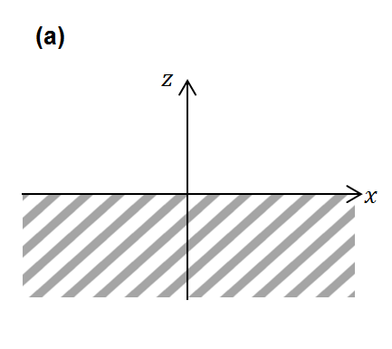 Figure 1
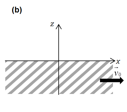 Figure 1
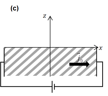 Figure 1
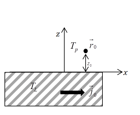 Figure 1
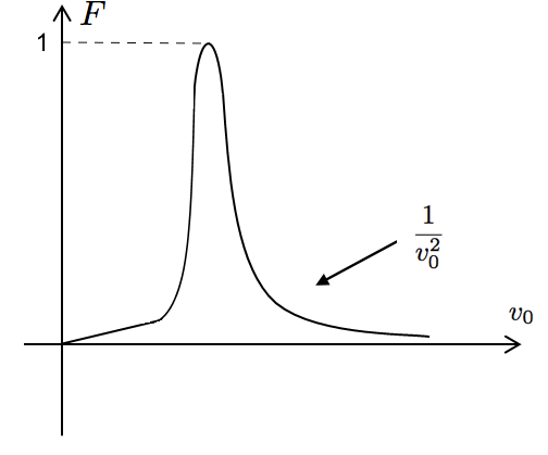 Figure 2
Peer Reviews
No public reviews on file for this paper yet. If you reviewed it on a platform where reviews are public (OpenReview, ICLR, NeurIPS, ICML), you can paste yours below so the community can read it here.
Videos
No videos yet. Explain this paper in a talk, walkthrough, or lecture? Add one.
Fluctuation induced forces in the presence of mobile carrier drift
Boris Shapiro
Department of Physics, Technion-Israel Institute of Technology,
Haifa 32000, Israel
Abstract
A small polarizable object (an atom, molecule or nanoparticle), placed above a medium with flowing dc current in it, is considered. It is shown that the dc current can have a strong effect on the force exerted on the particle. The Casimir-Lifshitz force, well studied in the absence of current, gets modified due to drifting mobile carriers in the medium. Furthermore, a force in the lateral direction appears. This force is a non-monotonic function of the drift velocity and its maximal value is comparable with the Casimir-Lifshitz force. If the temperatures of the medium and the particle are different, this lateral force can be directed along the current (drag) or in the opposite direction (anti-drag).
I Introduction
All bodies are surrounded by a fluctuating electromagnetic field, due to the random motion of charges inside a body. When a second body is placed in the vicinity of the first one, fluctuation-induced (Casimir-Lifshitz) forces appear between the bodies. These forces are of great relevance in chemistry, nanotechnology and biology [1, 2]. Much of the recent work on the fluctuation-induced forces, as well as on the related phenomena of near field heat transfer and the noncontact friction, deals with systems out of equilibrium (for some reviews see [3, 4, 5, 6, 7, 8, 9]). One should distinguish among several out-of-equilibrium situations :
- (i)
Different parts of the system have different temperatures but there is no relative motion between those parts (a hot body embedded into the cold environment is the simplest example of such situation [9, 10, 11]). Under such conditions the Casimir-Lifshitz forces will be modified, as compared to their equilibrium value [3, 4, 5, 6, 7, 8, 12, 13, 14, 15, 16, 17]. 2. (ii)
Different parts of the system are in relative motion. For instance, two macroscopic plates, separated by a vacuum gap, move one on top of the other. Another example is an atom (or a nanoparticle) moving above a macroscopic plate. Relative motion between bodies affects the Casimir-Lifshitz forces and, in particular, leads to dissipation and noncontact friction. This kind of problems was considered by many authors ([3, 4, 5, 6, 7, 8, 18, 19, 20, 21, 22, 23] and references therein), with rather controversial results (see Ref [7] for various contradictions and inconsistencies in the literature). 3. (iii)
There is no relative motion between parts of the system but some of the parts are subjected to a dc electric current [24, 25, 26, 27, 28] . The simplest example is to consider a semiconducting plate, with a dc current flowing in it, and ask how this current affects fluctuations of the electromagnetic field inside and outside the plate. This problem has been considered in [24, 25]. In the present paper we further elaborate on electromagnetic field fluctuations in the presence of carrier drift and, in particular, calculate the fluctuation force acting on an atom, or a nanoparticle placed above a sample with a dc current in it.
Let us stress that setups (ii) and (iii) are quite different- a fact not sufficiently appreciated in the literature. For one thing, the dc current in the sample produces a stationary (time independent) magnetic field which affects the atomic spectrum and, if inhomogeneous, exerts a force on the atom as a whole. More importantly, the fluctuation-induced forces in the two setups are not the same. The point is that in setup (iii) the mobile carriers are in motion (in the laboratory frame) while the lattice is fixed. Therefore the spontaneous fluctuations originating in the sub-system of the mobile carriers will be Doppler shifted with respect to those residing in the lattice. Moreover, in the presence of drift it is generally not even possible to assign a definite temperature to the mobile carriers, which makes the existing theory of the fluctuation-induced forces inapplicable. The purpose of this work is to study the effect of carrier drift on the fluctuation forces exerted on a small polarizable object (an atom, molecule or a nanoparticle).
The organization of the paper is as follows: In Section II we define the model and discuss how the fluctuational electrodynamics (Rytov’s theory) should be modified in the presence of mobile carrier drift. Section III is devoted to the properties of the fluctuating field, outside the sample with drifting carriers. In Section IV a particle is introduced, above the surface of a medium with drifting carriers, and the forces acting on the particle (both in the lateral and in the normal direction) are calculated. Various specific examples are presented in Section V and the conclusions are summarized in Section VI.
II Fluctuational Electrodynamics in the Presence of Carrier Drift
We consider a conducting medium, e.g., a semiconductor, containing mobile carriers with charge , effective mass and equilibrium concentration . When a dc voltage is applied to the sample, the carriers acquire some drift velocity , so that there is a steady state dc current . On top of this stationary drift there are fluctuations of the carrier and current density which cause fluctuations of the electric field. We designate the fluctuating part of these quantities as , and , respectively. Thus, for instance, the total current density is . The fluctuating part of the electric field is of particular interest because, unlike and , it exists also outside the sample and exerts forces on nearby objects. It should be emphasized that accounts only for the motion of the mobile carriers. In addition, there are fluctuating polarization currents due to the lattice. We briefly recapitulate the main equations of the theory, following with some modifications Ref [25].
The relation between and , in the frequency-wavevector domain is
[TABLE]
where summation over is implied. The conductivity tensor is defined with respect to the non-equilibrium steady state, i.e., it connects quantities fluctuating on top of the stationary current flow. That is why, even for an intrinsically isotropic medium, is a tensor depending not only on but also on . The dependence on occurs because the fluctuations are carried away by the flow, thus producing a non-local response (spatial dispersion). Adding the conduction current, Eq (1), to the fluctuating polarization current of the lattice yields the fluctuating displacement
[TABLE]
where is the lattice dielectric function which can depend on but not on . Eq (2) defines the dielectric tensor which controls the dynamics of electrical fluctuations in the medium. The form of depends on the specific system or model. We assume here Drude model, with drift, which is a special case of the more general hydrodynamic model (see Eq(11) of [25] with the thermal pressure term neglected) :
[TABLE]
where is the collision frequency of the mobile carriers, , and has been separated into the real and imaginary parts.
In our dealing with fluctuations we use Rytov’s method in which random Langevin sources are introduced into the Maxwell equations, similarly to what is done in the theory of Brownian motion. These random sources play the role of "external" currents and charges in the Maxwell equations and, if their correlation functions are known, one can compute the correlation function for various components of the electromagnetic field. We shall be interested in fluctuational phenomena close to the surface of the sample and neglect the retardation effects. In this limit the electromagnetic field is rotationless, , and Rytov’s fluctuational electrodynamics reduces to the Poisson equation supplemented by the Langevin sources. In the bulk of the sample this equation is
[TABLE]
where , are the Fourier transforms [29] of the potential and of the random Langevin sources , and
[TABLE]
Thus, the tensorial dielectric function in Eq (3) reduces to a scalar. (If the retardation effect were taken into account, then the full dielectric function, Eq (3), would come into play.) This expression has a simple interpretation. The dielectric function relates the displacement and the field in a longitudinal wave. If the wave propagates in the direction of flow, , then there is a Doppler shift of the wave frequency. There is no such shift if the propagation direction is perpendicular to . Note that only the plasma component of undergoes the Doppler shift, while the lattice component remains the same as in equilibrium.
For a system at equilibrium () the correlation function of the random sources is determined by the fluctuation-dissipation theorem [10, 11] :
[TABLE]
with
[TABLE]
where denotes thermal and quantum average, is the temperature of the system and is the imaginary part of its dielectric function [Eq (5) with ()]. Eq (6) defines the spectral densities , , and Eq (7) contains the essence of the fluctuation-dissipation theorem. Strictly speaking, , , , etc., should be understood as quantum-mechanical operators and various correlation functions should be properly antisymmetrized. These changes, however, would be only "cosmetic" and would not affect the final results. The point is that in the RHS of Eq (7) the correct quantum mechanical spectral density is given. With this ceavet, Rytov’s theory becomes essentially classical [30].
Since our system is out of equilibrium (), there is no general prescription for writing down the correlator of the random sources . However, under some conditions, it is possible to do so. As far as the lattice is concerned, the use of the fluctuation-dissipation theorem is justified because the lattice, even in the presence of an electric current, is usually close to equilibrium, i.e., the phonon distribution is close to Bose-Einstein. More precisely, the lattice is in internal equilibrium with some temperature , generally different from the environment temperature. Such internal equilibrium is a sufficient condition for applying the fluctuation-dissipation relation, as is indeed done in all the work where Casimir-Lifshitz forces or heat flow between bodies at different temperatures are considered. Thus, for the random sources originating in the lattice one can use the equilibrium theory, Eqs (6), (7), with replaced by [25, 31, 32]
[TABLE]
Similarly, in order to apply the fluctuation-dissipation theorem to the drifting plasma one should require that the plasma is in internal equilibrium, in its own frame of reference. This happens, for instance, at low drift velocities, when the electron distribution is close to Fermi-Dirac (or Bolzmann), with the temperature of the lattice. The more interesting example is the case of large drift velocities when, due to strong mutual interactions, the electronic system undergoes rapid internal thermalization, with a temperature higher than that of the lattice ("hot electrons"). We assume that the condition of internal equilibrium with some temperature is satisfied. In this case the random sources residing in the plasma are controlled by the imaginary part of the last term in Eq (5). Denoting this term by , where , we can write the fluctuation-dissipation theorem as
[TABLE]
The important difference between the Eqs (8) and (9), besides the trivial replacement of , by , , is that the frequency appears in Eq (9), i. e., the spontaneous creation of the fluctuations is now affected by the drift: the frequency of the fluctuations, as measured in the laboratory frame, is Doppler shifted. Let us note in this context that, while the electronic part of the dielectric function depends on the Doppler shifted frequency , the lattice part depends on the "bare" frequency . Therefore the problem of fluctuations in the presence of carrier drift is not equivalent to that for a moving sample. Only if one makes the additional assumption that do the two problems become equivalent (provided that the drifting electrons are in an internal equilibrium, which is in itself a rather strong assumption).
The two contributions to the spontaneous random sources [Eqs (8), (9)] are, of course, uncorrelated since they originate in two different subsystems- the lattice and the electron plasma. These equations, together with the Poisson equation and the expression for the dielectric function, Eq (5), allows us to treat fluctuations of various quantities, both inside and outside the medium with current, in the quasistatic limit (to include the retardation effects one has to replace the Poisson equation by the full set of Maxwell equations). Throughout the paper we discuss separately two limiting models, when either the lattice or the plasma make the dominant contribution to the fluctuations. While in principle it would be possible to consider the general situation, when both components make a comparable contribution, this would make the already combersome equations even more complicated and would only blur the basically simple physical picture.
Later, when considering the phenomena near a planar surface of the medium, we shall need Eq (4) in a somewhat different form. Assuming that the velocity vector is in the
- plane , i.e., does not depend on , we can transform Eq (4) back to space, in the direction, obtaining
[TABLE]
where denotes the transverse (in-plane) wave vector and is the Fourier transform of with respect to time and the - coordinates (the same for ). This -representation is convenient for handling the planar geometry. The spectral densities of the random sources, Eqs (7,8,9), should be also transformed to the -representation. For instance, Eq (8) becomes
[TABLE]
and similarly for the other spectral densities.
III Fluctuations of the Electric Potential Near the Surface
We consider a medium occupying half space while the other half is vacuum. The random charge sources produce evanescent electric fields near the surface (in addition to the radiation which we do not consider within our quasi-stationary, non-retarded approximation) and we are interested in various correlation functions for the potential and field. We shall consider three different setups, see Fig 1. Although case (a) has been studied long ago [9, 10, 11, 33, 34] and case (b) is simply related to (a), we discuss briefly also these two cases. The correlation functions obtained in this section will serve as building blocks in calculation of the fluctuation-induced forces in the next section.
Case (a) : The equilibrium dielectric function is (Eq (5) with )
[TABLE]
and we have to solve Eq (10) with this expression for . If one defines the Green’s function
[TABLE]
then the formal solution of Eq (10) is
[TABLE]
The solution of Eq (13), with the source inside the medium , the observation point outside and the standard boundary conditions for and its normal derivative at , is
[TABLE]
Since in equilibrium the lattice temperature is the same as the electron temperature, we can leave to denote the equilibrium temperature of the sample. Then, using (14),(15) and (11) (with insted of ) one obtains after some algebra:
[TABLE]
with
[TABLE]
Expression (17) factorizes into the -dependent and - dependent parts. The Fourier transform from to immediately yields
[TABLE]
The correlation function is obtained from (18) by multiplying it by the factor . This is the general rule, for any pair of fluctuating variables, and it follows from the stationary character of the fluctuations.
Correlation functions for various components of the electric field can be obtained from Eq (18) by differentiation. Some examples can be found in the above cited literature. For instance, differentiating Eq (18) with respect to and and setting at the end , one obtains
[TABLE]
i.e., when the surface is approached, the energy density increases as - the well known rule. This rule breaks down, of course, for sufficiently small , either because of spatial dispersion effects or simply because the macroscopic theory becomes inapplicable at atomic distances.
Case (b): The medium is now moving, in the laboratory frame, with velocity in the direction. In the frame moving with the medium all the relations derived above for case (a) remain of course valid, if the coordinates and frequency refer to that frame. It is immediate to translate the results to the laboratory frame. If we denote by some correlation function at equilibrium (i.e., in the rest frame of the sample), then the correlation function in the laboratory frame is simply . This relation holds in the non-relativistic limit, , assumed in the present work, and it implies that the Fourier transform is obtained from by replacing with . For instance the spectral density for a moving sample, as viewed from the laboratory frame, is given by the same expression as in the right-hand-side of Eq.(17) but with instead of . Note, though, that this replacement results in a complicated, non-factorizable function of and , and no simple expression in real space, comparable to Eq (18), can be obtained. We will not elaborate on this case further but move on to
Case (c): Here the sample is at rest but the electron subsystem moves with respect to the lattice with velocity , producing a dc current density . We do not specify the model for the lattice but just describe it by the lattice constant . The subsystem of the mobile carriers is described by the Drude model with drift, Eq (5).
In the limit of small collision frequency (the collisionless plasma model) the Langevin sources originating in the lattice dominate over those in the electronic subsystem. Taking the latter as “noiseless” and assuming the lattice in equilibrium, we can study the fluctuations using Eqs. (10),(11) with
[TABLE]
This model has been considered in [25]. An unnecessary approximation was introduced there at an early stage of the calculation. Here we present a somewhat different approach.
In fact, in - representation (i.e., Fourier transform in the - plane but not in the - direction) the calculation is straightforward and almost identical to case (a). The only difference is that the dynamics of the fluctuations is now controlled by the -dependent dielectric function in Eq (20), so that instead of (17) we have
[TABLE]
and the desired spectral density is
[TABLE]
Because of the dependence of the integrand in (22) does not factorize, as it did in case (a), and no simple analytical expression can be obtained. For small drift velocities one can expand in powers of . The first power does not contribute to (22) due to symmetry. The second power contributes, e.g., to the quantity in Eq (19), a term proportional to This follows from a simple power counting: an extra factor in the integrand contributes an extra term upon integration over .
It is worthwhile to mention an interesting qualitative effect due to the drift. In equilibrium the spectral density, Eq (19), has a sharp maximum at the frequency of the surface plasmon , when the factor becomes close to zero [9]. In the presence of drift we have instead of , i.e., surface plasmons acquire dispersion and, upon integration over , the peak in gets broadened.
Let us write down a useful spectral function which will be needed later:
[TABLE]
This result is obtained from Eq (22) [with Eq (21) inserted] by differentiating with respect to the pairs of variables and adding the corresponding expressions.
This concludes our discussion of the case when the lattice is the dominant source of noise. In the opposite limit the spontaneous random sources occur predominantly in the electron plasma. The appropriate dielectric function now is
[TABLE]
and the appropriate spectral density for the spontaneous random sources is given in Eq. (9) so that instead of Eq (21) we have
[TABLE]
This equation, unlike Eq (21), contains not only in the dielectric function but also in the argument of the coth. Therefore the small velocity expansion has now a different structure: The first non-vanishing term is still quadratic in the parameter but now one power can come from the coth-function. Thus, the result will contain first derivative of the dielectric function, in addition to a term with the second derivative.
IV Fluctuation - Induced Forces
Consider an electric dipole, with dipole moment , subjected to a space and time-dependent electromagnetic field . The size of the dipole is assumed to be much smaller than the characteristic wave length of the field (a “point dipole”). The dipole can rotate or vibrate but it does not move as a whole, i.e., it can be assigned a fixed position and an arbitrary time dependence . Under such conditions the dipole experiences an electric force ( is set equal to after differentiation) and the Lorenz magnetic force , where is the velocity of the positive charge of the dipole (and similarly for ). Thus, the magnetic force can be written as . Using the vector identity , one can write the total force as [35]
[TABLE]
In our problem the dipole moment and the fields are fluctuating quantities and, since the fluctuations are stationary, the last term in Eq (26) disappears upon averaging. We are left with the gradient term
[TABLE]
where, again, setting after differentiation is implied. This equation holds also for a dipole in motion and it serves as the starting point for calculating the fluctuation-induced forces [5, 8].
We now consider an atom, or a nanoparticle, or any entity with polarizability and size smaller than the relevant wavelength of the electromagnetic field (we use below the generic term “particle”). We allow for the particle temperature to be different from the sample temperature . The particle is placed at a distance above the sample surface (see Fig. 2 for a schematic setup).
The force acting on the particle consists of two parts:
- (i)
The fluctuating field emerging from the sample induces a dipole moment in the particle. This emerging field, which is just the field considered in the previous section, is often called “free” or “spontaneous” and will be designated as . Interaction of this field with the dipole moment induced in the particle is responsible for the first part, , of the force. 2. (ii)
The particle itself induces a fluctuating electric field in the environment, due to the spontaneous fluctuations of its dipole moment. We denote the latter by and the corresponding field by . This field acts back on the particle, giving the second part, , of the force.
Thus, Eq (27) splits into two parts, containing respectively and . Furthermore, since the particle polarizability is frequency dependent, one has to rewrite Eq (27) in frequency domain [36]:
[TABLE]
where has been used.
In the rest of this section we specialize to the case . Then the spectral density in the first term of Eq (28) is given, in somewhat different notations, in Eq (23), so that is obtained immediately, after applying and setting at the end. It is useful to split the integral over into two pieces: from to [math] and from [math] to . Switching the sign of the integration variables in the first piece, and using the conditions , , , we finally obtain the following expressions for the and - component of (the -component is zero) :
[TABLE]
[TABLE]
where is defined in Eq (20), , are the real and imaginary parts of , and . Since both the particle and the sample are at rest, it is natural that and depend on but not on (no Doppler shift). The Doppler shifted frequency enters only into the electronic part of which controls the dynamics of the fluctuations.
We now turn to the second term in Eq (28). First, one needs to compute the field induced by the spontaneous fluctuations of the particle dipole moment . To this end we introduce the Green’s function as a solution of the Poisson equation for a unit charge at point . Then the electric potential created at point by the “point dipole” and the electric field of that dipole are given by
[TABLE]
so that
[TABLE]
where labels the components and summation over indices is implied. The Green’s function can be written as
[TABLE]
where satisfies
[TABLE]
This is essentially the same as Eq (13), with instead of , but now we have both the source and the observation point above the sample surface, i.e., .
There is an apparent difficulty here, namely: , being a response to a point source, is singular at , and so is for . Since in Eq (28) we have to further differentiate the expression in Eq (32) with respect to and then set , we end up with a meaningless singular expression. This problem is well known in the theory of Casimir - Lifshitz forces (see, e.g., [3]) and the remedy is to make the standard subtraction of the vacuum Green’s function , Thus, the physical Green’s function is or the Fourier transformed , where is obtained from by replacing by unity. The result is:
[TABLE]
The last piece of information that we need to complete the calculation is the expression for the spectral density [37]
[TABLE]
where an isotropic particle, with temperature has been assumed. Putting all pieces together, and using we obtain the following expression for the components of :
[TABLE]
[TABLE]
where and are the real and imaginary parts of , Eq (35). The total force acting on the particle is the sum of and . In the next section we consider some specific examples.
V Fluctuation - Induced Forces: Summary, Discussion and Examples
Let us summarize our general results for the fluctuation-induced forces, acting on a particle in the presence of drifting mobile carriers in the medium. The medium is described by the Drude model with drift, Eq (5), and two opposite limits were considered:
Model 1: The dominant contribution to the spontaneous random sources comes from the lattice and dissipation in the electron plasma is neglected. The dielectric function of the model is , Eq (20).
Model 2: The dominant contribution comes from the electron plasma and dissipation in the lattice is neglected. The dielectric function of the model is , Eq (24).
The main reason for introducing these two limits, rather than dealing with the general model, Eq (5), is that the frequency of the fluctuation sources originating in the drifting plasma is Doppler shifted with respect to those originating in the lattice. Thus, while it is easy to write down the spectral density of the sources for the general case (this is just the sum of Eqs (8) and (9)), it would make the resulting expressions for the forces even more cumbersome and more difficult to analyze. We therefore prefer to clarify the basic physics of the problem using the two limiting models.
Let us first return to "Model 1". Since , we have
[TABLE]
This identity enables one to write Eqs (29, 30) in terms of . Adding to Eqs (29, 30) their counterparts in Eqs (37, 38) gives the final expressions for the components of the total force in "Model 1":
[TABLE]
[TABLE]
Let us clarify a bit these expressions, starting with Eq (41). This normal-to-surface component is the generalization of the standard, equilibrium Lifshitz force between a particle and medium [37]. The generalization includes the effect of carrier drift in the medium and it allows for different temperatures of the medium and the particle. The first part of the force, proportional to , is due to the fluctuating field in the medium acting on the particle. The particle itself is "passive", hence . In the second part, proportional to , the fluctuating field originates in the particle and, after being "reflected" from the medium, acts back on the particle. Here the medium is passive, hence . Note that both -functions have in their argument the unshifted frequency . This is because in "Model 1" the spontaneous fluctuating sources of the medium reside in the lattice, which is at rest in the laboratory system (the particle is at rest as well). The Doppler shifted frequency appears only in which contains information on the effect of the drift on fluctuation dynamics.
The structure of Eq (40) is different. This equation describes the dissipative "drag" force, due to the current flow in the medium. For this force to exist both and (i.e., ) must differ from zero. However, the "active" part of the system can be distinguished from the "passive" one by looking at the argument of the . The first term in Eq (40), proportional to , is due to the random sources in the medium, i.e., the medium is the emitter while the particle is the absorber (and vice versa for the second term).
To switch to "Model 2" the following replacements are required in Eqs (40,41): The lattice temperature is replaced by the temperature of the electron plasma and is changed to , which is defined in Eq (35), with subscript instead of 1. Furthermore, since the spontaneous sources in the medium now originate in the drifting plasma, the frequency in the argument of the corresponding -function should be Doppler shifted. Thus, the counterparts of the Eqs (40,41) for "Model 2" read as:
[TABLE]
[TABLE]
The above expressions for the forces resemble those obtained in the literature for the problem of non-contact friction, experienced by a particle moving above a medium at rest [4, 7, 8] (or, alternatively, the problem of "drag" exerted on the particle by a moving medium). Our problem, however, is different and so are the results. Since in our setup the plasma component is moving with respect to the lattice, the dielectric function governing dynamics of the fluctuations is in general a complicated function of and . In addition, the frequency dependence of the random sources in the drifting plasma is different (Doppler shifted) with respect to those in the stationary lattice. Due to these factors the results are sensitive to the details of the model and can be quite diverse. For instance, in "Model 1" there are no "drag" at all, if the temperature of the sample and the particle are equal, see Eq (40) with . This is because, as has been mentioned above, in "Model 1" the random sources, both in the medium and in the particle, are at rest. Only the dielectric function is affected by the drift. Therefore the situation is the same as in equilibrium, but with a modified, -dependent dielectric function of the medium.
To obtain specific results we need an explicit expression for the particle susceptibility . We shall use the most simple, "generic" expression applicable to a two-level system:
[TABLE]
where is the resonance frequency of the excitation and is the decay rate. This expression is valid for an atom or a molecule when a single excitation is of importance. It is also applicable to a metallic or semiconducting (spherical) particle, in which case is equal to the cube of the radius of the sphere and is the frequency of the localized surface plasmon [38]. (Here is the plasma frequency of the material of the particle). For a dielectric nanoparticle one may have some phonon mode or a phonon-polariton, instead of a plasmon. The value of depends on the nature of the particle and can vary over a few orders of magnitude, say, between and .
In the weak dissipation (small ) limit the imaginary part of is often approximated as
[TABLE]
However, one should keep in mind that, when is integrated with some function of frequency , the "-function approximation" is valid only if is not negligibly small. Otherwise the integral will be dominated not by the peak of the Lorenzian in Eq (45) but by some other region of frequencies where is significant (albeit the Lorenzian is small). Below we shall encounter a situation where the integral is dominated by small frequencies and, correspondingly, the low-frequency expansion
[TABLE]
will be used.
The same remark applies to , defined in Eq (39) (and similarly for , with instead of ). In the small dissipation limit, the general expression can be approximated, in some cases, by the -function
[TABLE]
It is assumed here that the relevant frequencies are far from the resonant frequencies of the lattice and can be treated as a constant, hence and are combined into a single argument . In the -function approximation there is no difference between and , so that the subscript has been removed. Note that Eq (47) does not explicitly contain or although some dissipation, albeit infinitely small, is essential. Since, however, in reality the dissipation is finite, the -function approximation has its limitations and, in particular, below we shall need the small frequency approximation
[TABLE]
We are now in a position to work out some examples of the drift effect on fluctuation induced forces. The most interesting effect is the appearance of the aforementioned drag force.
V.1 Drag force in "Model 1"
In this model the drag force on a particle appears only if and are different, see Eq (40). Note that if and are reversed, the force changes sign, i.e., drag (force in the direction of the current) turns into "anti-drag" (force in the opposite direction)[39]. Let us calculate the force using the -approximation for , Eq (45). This is justified because the integral is dominated by the peak of the Lorenzian. The -function takes care of the integral over in Eq (40), and we have to address the integral over , with . The latter quantity is defined in (39). Since is a small number, has a sharp maximum when . This happens at . One can try to approximate the Lorenzian function in Eq (39) by the -function, Eq (47), thus obtaining
[TABLE]
In order to see how good is this approximation one must keep in mind that, due to the exponential factor, the integrand in Eq (40) has a sharp cutoff at , hence the -approximation will be justified only if at least one of the roots is below the cutoff- otherwise the contribution from the peak of is exponentially small (we assume here that both roots are positive). The -approximation is always justified for sufficiently large but the precise criterion depends on the values of , and . For an atom is typically much larger than of the semiconducting medium but for a large molecule or a nanoparticle (dielectric or semiconducting) the two frequencies can be of the same order. We assume that is few times larger than and obtain the condition for the validity of the -approximation. The force is then estimated from (40) as
[TABLE]
In this regime drops as under increase of the drift velocity. It achieves its maximum value for , at which point the -approximation breaks down. For a hot medium, (, and a "cold particle", (, this maximum value is of the order of which is comparable with the equilibrium Casimir-Lifshitz force.
In the opposite case of small drift velocities the -approximation breaks down and the integral is dominated by small . should then be expanded near the point with respect to . The expansion has a linear term, unless = when the first correction is quadratic in . We assume to be well away from this point, taking few times larger than . The first contribution to comes then from the linear term which, after substitution into (40) and integration over , yields
[TABLE]
Note that the two expressions, Eqs (50) and (51), do not match at which means that there is an intermediate region where sharply increases, interpolating between the small and large velocity limits. The overall behavior of , as a function of , is schematically scetched in Fig. 3. If one takes and , then the critical drift velocity for which the maximal value of the force is reached, is . Although this is comparable to a typical saturation velocity in semiconductors, reaching the maximum force value and, morover, observing the decay might well be unrealistic. In addition to the very small and very large needed for such observation, it is not at all clear that under such extreme conditions the electron plasma can be characterized by a temperature.
V.2 Drag force in "Model 2"
The expression for the force is given in Eq (42). Due to the Doppler shifted frequency in the argument of the first , the force exists also when the medium and the particle have equal temperatures, , and we concentrate on this case. The most interesting limit is ("quantum drag"). In this limit the difference between the two functions in Eq (42) is equal to for and it is zero otherwise (recall that must be positive). Thus, Eq (42) reduces to
[TABLE]
One might be tempted to approximate the Lorenzian by the -function in Eq (45). This. however. is possible only if the upper limit in the integral over is larger than the center of the Lorenzian peak. Since the relevant values of are smaller than , we arrive again to the parameter (. Only if this parameter is large can one justify the "-approximation".
For small value of the upper limit in the integral over frequency is smaller than and one should use the low-frequency expressions for and , Eqs (46)) and (48)) respectively. Note that in the integration region over the frequency, is negative, and so is . The integral over is proportional to and the force is of the order of
[TABLE]
For large the main contribution to the integral over frequencies in Eq (52) comes from high frequencies, , and the -approximation for is valid. Thus, first one integrates over and then over , using the -approximation for . Due to the restriction , is now negative and its argument has only one root, namely, . Assuming again that is few times larger than , we arrive to a simple estimate
[TABLE]
The fundamental difference between this expression and its counterpart in "Model 1", Eq (50), is that Eq (54) was derived in the zero-temperature limit, when Eq (50) (as generally for equal temperatures of the particle and the medium) is zero. The qualitative behavior of in Eq (54), as a function of , is similar to that shown in Fig.3, although the initial slope is less steep (proportional to instead of being linear). The maximal value of the force, , is achieved for (in this estimate we take to be few times larger than and assume ). This force is of the same magnitude as the usual Casimir-Lifshitz attraction force between a particle and a medium, in equilibrium.
V.3 Effect of drift on
Unlike the lateral force , the normal (Casimir-Lifshitz) force exists already in the equilibrium. This force, however, is affected by the drift of the mobile carriers. To concentrate exclusively on the effect of drift we take and consider "Model 1", Eq (41). In this case the integral over frequencies can be reduced to a Matsubara sum, in spite of the fact that the system is not in equilibrium. Indeed, becomes a common factor for both terms in Eq (41) and they can be combined into an expression containing which results in a Matsubara sum
[TABLE]
where () and the prime on indicates that the term should be taken with a factor . In equilibrium and are real so that the sign "Re" in front of the sum becomes redundant. In the presence of drift, however, acquires -dependence and becomes complex on the imaginary frequency axis. Neglecting small dissipation, we have
[TABLE]
where again , which is generally a function of frequency, is treated here as a constant.
In the low-T limit, i.e., (these are frequency scales on which and changes significantly). the sum can be replaced by an integral according to the rule , i.e.,
[TABLE]
One can compute the correction to the force, due to carrier drift, by expanding in powers of . The zero-order term corresponds to equilibrium, when does not depend on and
[TABLE]
For this coincides with the well known expression for the attraction force between a "two-level atom" and a collisionless plasma [37]. The coefficient in Eq (58) accounts for the effect of the lattice. The first order correction, i.e., the one linear in , does not contribute to the force. The second order corrrection
[TABLE]
contributes to Eq (57) the term
[TABLE]
Assuming that is not close to and taking, as before, to be few times larger than , one recovers the same condition for the validity of the expansion.
Eq (60) can be derived directly from Eq (41), without using the Matsubara representation, although the latter is more flexible when it comes to non-negligible dissipation and arbitrary temperatures. The transformation of the expression in Eq (41) to the Matsubara sum was possible because in "Model 1" (and for ) the spontaneous fluctuation sources are in equilibrium at the same temperature, only the (noiseless) plasma component is in motion. This is not the case for "Model 2", where the sources originating in the moving plasma are Doppler shifted, so one has to work directly with the expression in Eq (43). For small drift velocities and in the weak dissipation limit, when the -approximation for and can be used, the calculation is quite straightforward and will not be pursued here. Instead, we briefly discuss the case when the sample and the particle have different temperatures but there is no drift. Then, for negligible dissipation, Eqs (41) and (43) become identical and the result is the same for either model:
[TABLE]
This is a slight generalization of the result obtained in [16] where , i.e., . This latter case is appropriate for the free electron gas model, while the expression (61) includes the effect of the underlying lattice. The constant can vary between [math] and , and for a typical semiconductor, in broad intervals of frequencies, it can be few tenths or even close to , so its effect is quite significant. The ()-term in (61) can become the dominant one. For instance, taking the low temperature limit, i.e., replacing the - factors by , and assuming , one obtains . This should be compared with for the electron gas model under the same conditions. The interesting feature, pointed out already in [16], is that, depending on the parameters of the model, the force can be either repulsive or attractive.
VI Conclusion
We have studied the fluctuation-induced forces acting on a small polarizable neutral particle (atom, molecule or a nanoparticle), located close to the surface of a conducting medium. It is shown that presence of a dc current (i.e., the mobile carrier drift) in the medium can have a significant effect on the forces. In particular, there appears a lateral force which can be in the direction of the current (drag) or in the opposite direction (anti-drag). This phenomenon is distinct from the well studied Coulomb drag [40], when current in a conductor induces a current (or voltage) in a nearby conductor. In our case the force is exerted on a small polarizable object, with a well defined excitation, at some frequency . This can be the resonant frequency of an atom or the frequency of a localized surface plasmon of a nanoparticle. The resulting drag force is a non-monotonic function of the carrier drift velocity and it reaches a maximal value at of the order of . The maximal value of the force is not small, in the sense that it is comparable to the normal (Casimir-Lifshitz) force in equilibrium.
Formulas for the forces, obtained in the present work, resemble those which appear in the theory of non-contact friction (item (ii) in the Introduction). The two problems, however, are different. In our problem both the particle and the sample are at rest, in the laboratory frame, only the mobile charge carriers are drifting. Our results depend on whether the random spontaneous sources reside predominantly in the lattice or in the electron plasma (Models 1 and 2, respectively). If dissipation in the lattice can be neglected (Model 2) and, moreover, is assumed to be constant, then the dielectric function of the medium (lattice + plasma) is a function of only and, since the random sources are located in the drifting plasma, the situation becomes as close as possible to the case of a medium moving as a whole. However to make the analogy complete one needs an additional strong requirement, namely, that the electrons in the drifting plasma could be considered as being in an internal equilibrium, with some effective temperature . Otherwise one cannot use Rytov’s theory for correlation functions of the random sources.
We limited our considerations to the simplest models and conditions and did not attempt possible generalizations and extensions, like treating the general case (Eq (5) with both and finite), or going beyond weak dissipation limit, or including the retardation effects. Finally, let us stress that the high drift velocities, needed to make the discussed effects visible, can be achieved only in materials with low carrier density, like semiconductors, ionic conductors or other types of "bad conductors".
VII Acknowledgement
Numerous instructive discussions with J. Avron, J. Feinberg, O. Kenneth and U. Sivan are gratefully acknowledged. I am indebted to G. Dedkov for sending to me his review, Ref. [8], prior to publication.
The reference list from the paper itself. Each links out to its DOI / PubMed record.
- 1[1] M. Bordag, G. L. Klimchitskaya, U. Mohideen and V. M. Mostepanenko, Advances in the Casimir Effect, Oxford Science Publications, 2009.
- 2[2] V. A. Parsegian, Van der Waals Forces: A Handbook for Biologists, Chemists, Engineers, and Physicists, Cambridge University Press, 2005.
- 3[3] G. Bimonte, T. Emig, M. Kardar and M. Krüger, Annuel Review of Condensed Matter Physics 8 , 7.1 (2017)
- 4[4] A. I. Volokitin and B. N. J. Persson, Rev. Mod. Phys. 79 , 1291 (2007).
- 5[5] F. Intravaia, C. Henkel and M. Antezza, in "Casimir Physics", Lecture Notes in Physics 834 (D. Dalvit et al, eds.).
- 6[6] M. De Kieviet, U. D. Jentschura and G. Lach, in "Casimir Physics", Lecture Notes in Physics 834 (D. Dalvit et al, eds.).
- 7[7] A. A. Kyasov and G. V. Dedkov, Arxiv: 1112.5619.
- 8[8] G. V. Dedkov and A. A. Kyasov, Fluctuation-electromagnetic interaction under the conditions of thermal and dynamical disequilibrium, Physics- Uspekhi (in Russian), 187 , 599 (2017).