Asymptotic Enumeration of Compacted Binary Trees of Bounded Right Height
Antoine Genitrini, Bernhard Gittenberger, Manuel Kauers, Michael, Wallner

TL;DR
This paper derives the asymptotic enumeration of compacted binary trees with bounded right height, using exponential generating functions and differential equations, addressing the growth complexity of these structures.
Contribution
It introduces a calculus on exponential generating functions for compacted trees of bounded right height, enabling asymptotic counting of these complex structures.
Findings
Asymptotic formulas for the number of compacted trees of bounded right height
Development of a differential equations approach for generating functions
Analysis of relaxed trees as a simplified model
Abstract
A compacted binary tree is a graph created from a binary tree such that repeatedly occurring subtrees in the original tree are represented by pointers to existing ones, and hence every subtree is unique. Such representations form a special class of directed acyclic graphs. We are interested in the asymptotic number of compacted trees of given size, where the size of a compacted tree is given by the number of its internal nodes. Due to its superexponential growth this problem poses many difficulties. Therefore we restrict our investigations to compacted trees of bounded right height, which is the maximal number of edges going to the right on any path from the root to a leaf. We solve the asymptotic counting problem for this class as well as a closely related, further simplified class. For this purpose, we develop a calculus on exponential generating functions for compacted trees of…
Click any figure to enlarge with its caption.
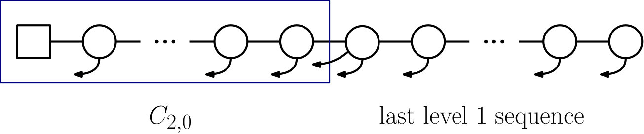 Figure 1
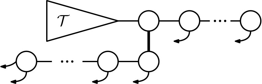 Figure 2
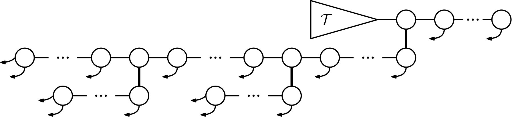 Figure 3
 Figure 4
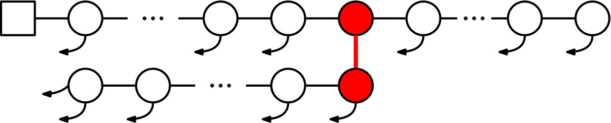 Figure 5
 Figure 6
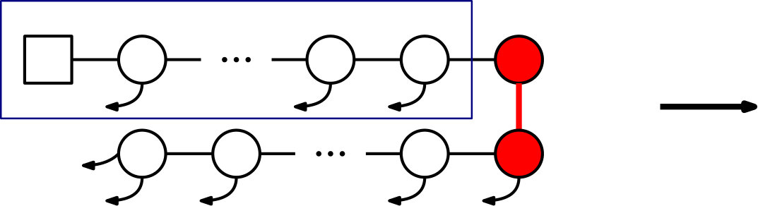 Figure 7
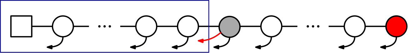 Figure 8
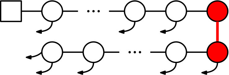 Figure 9
 Figure 10
 Figure 11
 Figure 12
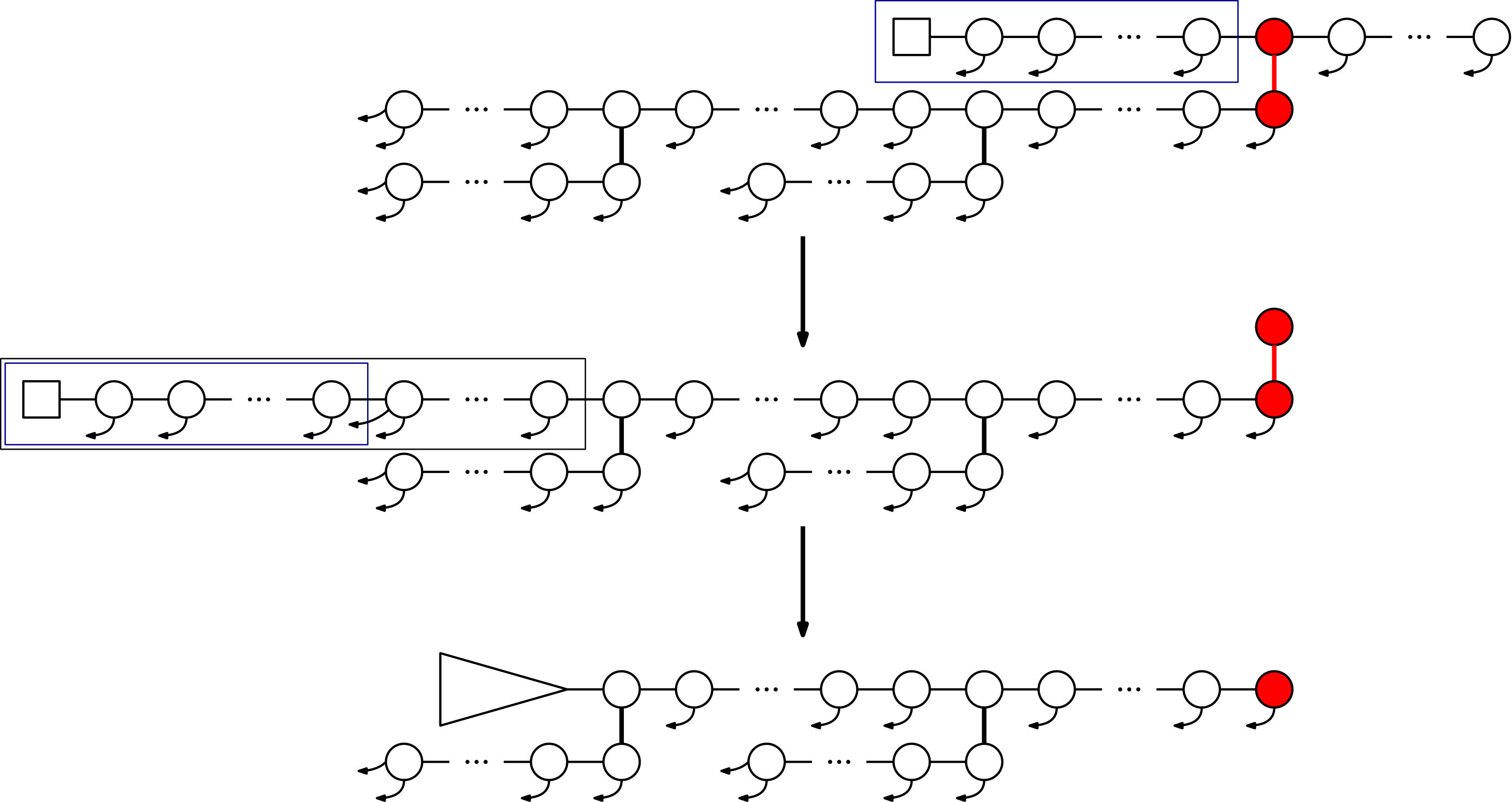 Figure 13
 Figure 14
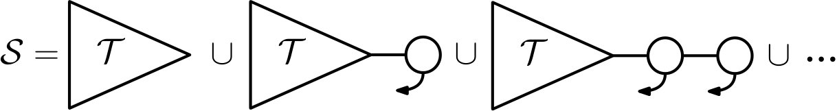 Figure 15
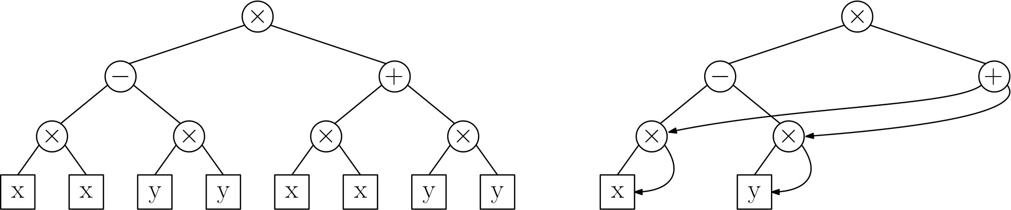 Figure 16
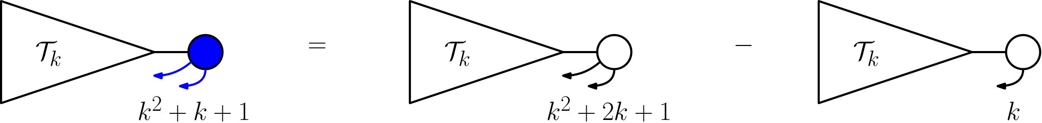 Figure 17
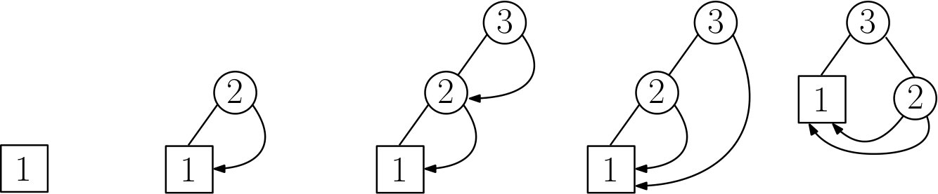 Figure 18
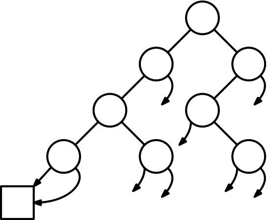 Figure 19
 Figure 20
 Figure 21
 Figure 22
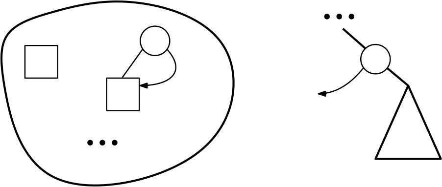 Figure 23
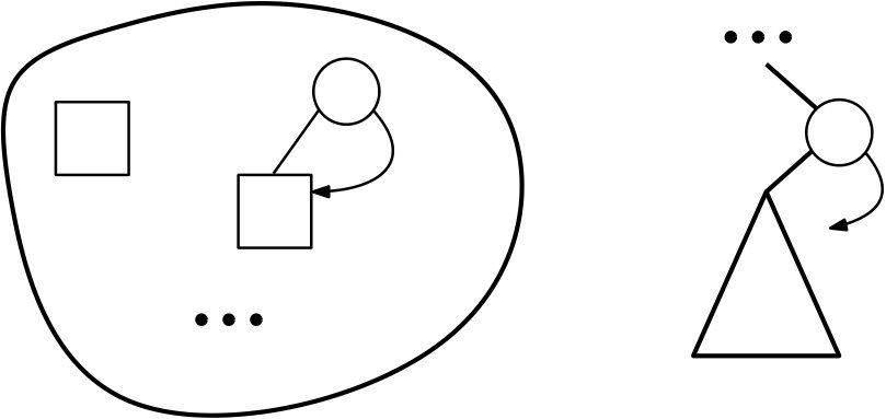 Figure 24
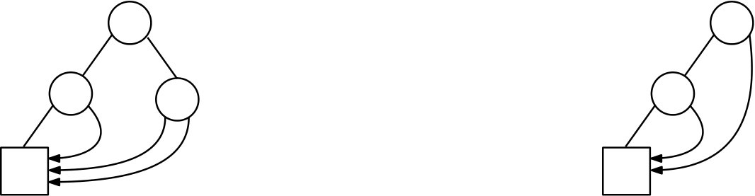 Figure 25
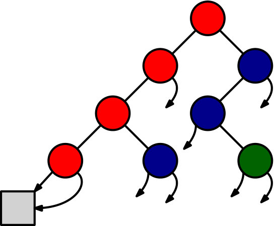 Figure 26
 Figure 27
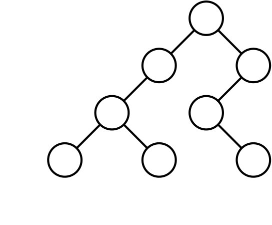 Figure 28
Peer Reviews
No public reviews on file for this paper yet. If you reviewed it on a platform where reviews are public (OpenReview, ICLR, NeurIPS, ICML), you can paste yours below so the community can read it here.
Videos
No videos yet. Explain this paper in a talk, walkthrough, or lecture? Add one.
Asymptotic Enumeration of Compacted Binary Trees of Bounded Right Height††thanks: This research was supported by the Austrian Science Fund (FWF) grant SFB F50-03.
Antoine Genitrini Sorbonne Universités, UPMC Univ Paris 06, CNRS, LIP6 UMR 7606, 4 place Jussieu 75005 Paris. [email protected]
Bernhard Gittenberger Technische Universität Wien, Wiedner Hauptstraße 8-10/104, 1040 Wien, Austria. {Bernhard.Gittenberger,Michael.Wallner}@tuwien.ac.at
Manuel Kauers Institute for Algebra, Johannes Kepler University, Altenberger Strasse 69, 4040 Linz, Austria. [email protected]
Michael Wallner*‡*
Abstract
A compacted binary tree is a graph created from a binary tree such that repeatedly occurring subtrees in the original tree are represented by pointers to existing ones, and hence every subtree is unique. Such representations form a special class of directed acyclic graphs. We are interested in the asymptotic number of compacted trees of given size, where the size of a compacted tree is given by the number of its internal nodes. Due to its superexponential growth this problem poses many difficulties. Therefore we restrict our investigations to compacted trees of bounded right height, which is the maximal number of edges going to the right on any path from the root to a leaf.
We solve the asymptotic counting problem for this class as well as a closely related, further simplified class.
For this purpose, we develop a calculus on exponential generating functions for compacted trees of bounded right height and for relaxed trees of bounded right height, which differ from compacted trees by dropping the above described uniqueness condition. This enables us to derive a recursively defined sequence of differential equations for the exponential generating functions. The coefficients can then be determined by performing a singularity analysis of the solutions of these differential equations.
Our main results are the computation of the asymptotic numbers of relaxed as well as compacted trees of bounded right height and given size, when the size tends to infinity.
**Keywords: **Compacted trees, Enumeration, D-finiteness, Analytic Combinatorics, Directed Acyclic Graphs, Chebyshev Polynomials.
††footnotetext: © 2020. This manuscript version is made available under the CC-BY-NC-ND 4.0 license http://creativecommons.org/licenses/by-nc-nd/4.0/
1 Introduction
Most trees contain redundant information in form of repeated occurrences of the same subtree††In the rest of the paper, a subtree of a given tree contains a root and all its descendants in the original tree. Such a substructure is sometimes called a fringe subtree.. In order to get an efficient representation in memory, these trees can be compacted by representing each occurrence only once. The removed subtrees are replaced by pointers which link to the shared subtree. Such structures are classically named as directed acyclic graphs or short as DAGs.
Flajolet et al., in their extended abstract [15], analyzed in detail the gain in memory of the compaction. Some proofs have been omitted and have not been stated later. This gap was closed in [10], where the framework was extended to other DAG structures and analyzed in the context of XML compression. Furthermore, Ralaivaosaona and Wagner extended in [27] the analysis of the gained memory to simply generated families of trees.
The latter two papers on the quantitative analysis of the compaction process, studied the transformation of a given set of trees of given size to the set of compacted trees in order to determine the average rate of compaction. We focus on a different aspect, namely the enumeration problem of compacted binary trees. On the one hand, enumerating combinatorial structures is important if one wants to understand shape characteristics of large random structures or for uniform random generation of those structures. On the other hand, the enumeration of particular classes of DAGs is in general a difficult problem which requires the extension of combinatorial methodology and is therefore interesting in its own right.
One of the difficulties in the enumeration of compacted binary trees lies in the fact that a compacted binary tree of size could arise from a binary tree whose size belongs to the whole interval . Thus, a brute-force approach is hopeless.
The first papers about the enumeration of DAGs appeared in the 1970’s. Robinson presented two distinct approaches [28, 30] based either on some inclusion-exclusion method or on Pólya’s enumeration theory [26]. Combining combinatorial arguments and analytic methods the asymptotic number of labeled DAGs was determined in [4], for connected structures then in [5]. The first investigation of shape parameters seems to go back to McKay [22]. Recently, enumeration results for many particular classes of DAGs can be found in the literature, see for instance [7, 8, 9, 16, 20, 21, 33, 34, 35], as well as investigations on the (random) generation of particular DAGs, see [3, 11, 23, 24].
A now classical way for enumeration is the use of generating functions. In this context, precisely for labeled structures (see paper [29]), Robinson designed generating functions of a very particular nature to solve an asymptotic counting problem concerning DAGs. The classical types of generating functions like ordinary and exponential ones were not suited for the problem.
We are facing the same problem in the enumeration of compacted trees. Indeed, due to the fact that compacted trees are unlabeled combinatorial structures, which are moreover closely related to plane trees, a treatment with ordinary generating functions will be the first choice. However, the fast growth of the counting sequence requires the use of exponential generating functions. In order to be able to get asymptotic results, we will confine ourselves to certain subclasses of the class of compacted trees as well as some related classes by relaxing certain conditions. Moreover, we will develop a calculus for exponential generating functions designed for these classes. Bounding the right height of our DAGs leads to a sequence of D-finite functions (see [19, 32] for introductions to the subject) for which it is possible to analyze their differential equations and obtain finally our main result. Likewise, in other enumeration problems for particular classes of DAGs bounding a certain parameter turned intractable recurrences into D-finite ones. Examples are the enumeration of certain classes of lambda-terms [7, 9, 8] or increasing series-parallel DAGs [6].
Plan of the paper
Our combinatorial structures are based on the fundamental properties of the compaction procedure. We will first analyze some properties of this classical procedure (linked to the common subexpression problem) in Section 2.
Then we will define the basic concepts and state our main results in Section 3, see Theorems 3.3 and 3.4.
Some basic observations concerning the structure of compacted trees will then be presented in Section 4.
These will help us to state a combinatorial and (most importantly) recursive specification of the problem in Section 5. A further important result is the derivation of a recurrence relation for the number of compacted binary trees, see Theorem 5.1. This recurrence is not classical at all, and we are not able to solve it explicitly.
Due to this fact, we follow yet a different approach in the remaining part of this work: We will use exponential generating functions to model our problem, as the superexponential growth rate of the counting sequence suggests, though we are dealing with unlabeled combinatorial structures. Therefore, a new calculus translating certain set operations for classes of compacted trees into algebraic operations of exponential generating functions will be developed in Section 6.
Section 7 is devoted to a simplified problem, the study of the counting problem of relaxed binary trees. These DAGs are in a sense compacted trees where the restriction of uniqueness on the subtrees is relaxed. In particular, compacted trees are a subset of relaxed binary trees. With the same methods as used on compacted trees we are able to derive a recurrence relation. However, this recurrence relation is as difficult as the first one for compacted trees.
A natural constraint for compacted trees seems to bound some specific depth limit, the so-called right height. This is the maximal number of edges directed to the right which appear on any path from the root to a leaf. In Section 7, the calculus developed in Section 6 enables us to derive a differential equation for the generating function of relaxed trees for each bound on the right height. This sequence of D-finite differential equations follows a rather explicit recursive scheme, presented in Theorem 7.10 which allows us to analyze the dominant singularities of the solutions of the differential equation for any . Eventually, this strategy is successful and we are able to determine the asymptotic number of relaxed binary trees of bounded right height.
Finally, in Section 8 we modify the results of the previous section to cover the case of compacted trees as well. Again, we derive a sequence of D-finite differential equations where, as in Section 7, the dominant singularities of the generating function are regular singularities of the differential equation. This allows us to extract the asymptotic behavior of the counting sequence, which contains irrational powers of . The necessary information is directly extracted from the differential equations. Except for the first few, they do not have closed-form solutions.
2 Creating a compacted tree
Many problems in computer science and computer algebra involve redundant information. A strategy to save memory is to store every instance only once and to point to already existing instances, whenever an instance appears repeatedly. In [15, Proposition 1] a compression algorithm was presented, and it was shown that for a given tree of size , its compacted form can be computed in expected time . However, such procedures have been known since the ’s (see [15, 13] and especially the “value-number method” in compiling [2, Section 6.1.2]). Figure 1 shows this procedure, which follows a top-down decomposition scheme (i.e. post-order traversal) of labeled binary trees. Every node (or actually the subtree whose root is the respective node) is associated with a “unique identifier” (uid). Two subtrees are equivalent if and only if the uid’s are the same.
We now give an example of the behavior of the procedure for an arithmetic expression.
Example 2.1: Consider the labeled tree necessary to store the arithmetic expression (* (- (* x x) (* y y)) (+ (* x x) (* y y))) which represents . The “Table”, built by the UID procedure, contains
[TABLE]
and the tree in its full and compacted version is shown in Figure 2. ■
Motivated by this procedure, based on a post-order traversal of the tree, we define an ad hoc DAG-structure, which we call a compacted binary tree, that encodes the result of the compaction of the tree. The trees under consideration are full binary in the sense that their nodes have either 0 or 2 children. Furthermore, in the definition we refer to subtrees: a fringe subtree or short subtree is the tree which corresponds to a node and all its descendants. In this paper we only consider such subtrees.
Definition 2.2**.**
A compacted binary tree is a DAG computed by the UID procedure from a given full binary tree. Every edge leading to a subtree that has already been seen during the traversal is replaced by a new kind of edge, a pointer, to the already existing subtree. The size of the compacted binary tree is defined by the number of its internal nodes.
In the sequel we will only consider full binary trees and their compacted forms. Thus, the term compacted trees means compacted binary trees. In Figure 3, we represent all compacted trees of size , and .
The subclass of DAGs we are interested in is strongly influenced by properties of trees. In particular, compacted trees are connected and plane. The out-degree††For the terms out- and in-degree, source, sink, and so on, we interpret an undirected edge as directed away from the root, in accordance with a node-child relation. of each node is equal to , except for the unique sink (leaf) for which it is [math]. Furthermore, there is a unique source, which is the root.
The latter properties are induced by the full binary tree structure. Next, we treat the specific properties of the UID procedure. The result of the algorithm strongly depends on the chosen traversal. In this case the post-order traversal is used – but one could also consider a different one. There are two important observations. First of all, it has an important consequence on the pointers:
Proposition 2.3**.**
In a compacted tree the pointers only point to previously discovered trees.
In other words, the ordering imposed by the traversal restricts the possible choices of the pointers.
Definition 2.4**.**
For any compacted tree of size , the spine is the structure (with nodes) obtained from the compacted tree by deleting all pointers and the leaf.
In the Figure 4, from left to right, we see a compacted tree (without details on the pointers) and its spine. Furthermore, every distinct subtree is stored only once. In terms of the corresponding compacted trees this translates into uniqueness of every subtree.
3 Main results
Before being able to state our main results we have to define further combinatorial classes. Indeed, the uniqueness condition for compacted trees caused some difficulties in their enumeration. So, we will first analyze a simpler class where we drop this condition.
Definition 3.1**.**
A relaxed compacted binary tree (short relaxed binary tree, or just relaxed tree), of size is a directed acyclic graph consisting of a binary tree with internal nodes, one leaf, and pointers. It is constructed from a binary tree of size , where the first leaf in a post-order traversal is kept and all other leaves are replaced by pointers. These links may point to any node that has already been visited by the post-order traversal.
Obviously, the notion of spine adapts to the class of relaxed trees.
In fact, let us give another way to interpret compacted trees: compacted trees are relaxed trees with the restriction that all nodes in the spine are the roots of unique subtrees of the full tree. Note that this condition does not hold for all relaxed trees. In particular compare Figure 5 for the smallest relaxed tree which is not a compacted tree.
The asymptotic enumeration of relaxed trees is still too complicated. We will derive recurrence relations for their counting sequence as well as for the counting sequence of compacted trees. In order to obtain asymptotic results, we restrict the right height.
Definition 3.2**.**
For any relaxed tree, we define its right height to be the maximal number of right edges on any path from the root to another node in the spine (of the relaxed or compacted tree under consideration). The level of a node is the number of right edges on the path from the root to this node.
Figure 6 introduces an example and a natural way of representing a relaxed tree in order to emphasize these notions. It proves convenient to rotate the trees by degrees.
Bounding the right height defines a sequence of classes which follows a recursive construction principle. We will eventually exploit this structure and obtain our main results, the asymptotic number of relaxed trees with internal nodes and the analogous result for compacted trees.
Theorem 3.3** (Asymptotics of relaxed trees with bounded right height).**
The number of relaxed trees with right height at most is for asymptotically equivalent to
[TABLE]
where is a positive constant which is independent of .
Theorem 3.4** (Asymptotics of compacted trees with bounded right height).**
The number of compacted trees with right height at most is for asymptotically equivalent to
[TABLE]
where is a positive constant which is independent of .
Therefore, we can also answer the question (at least asymptotically) of how many relaxed trees are actually compacted trees. Combining Theorems 3.3 and 3.4 we get the following result.
Corollary 3.5** (Proportion of compacted among relaxed trees).**
Let () be the number of compacted (relaxed) binary trees with right height at most . Then, for we have
[TABLE]
Thus, the number of compacted trees among relaxed trees for large is negligible. This result quantifies the restriction of uniqueness of subtrees in compacted trees.
4 On the structure of compacted trees
In this section we will discuss some basic observations concerning the structure of compacted trees. First note that pointers may point to nodes lying outside the subtree of the pointer’s start node (compare with Figures 2 and 3). Such subtrees of compacted trees cannot be compacted trees themselves. For this reason, we define the concept of c-subtrees.
Definition 4.1**.**
A c-subtree is the subgraph of a compacted tree induced by a node and all its descendants. A cherry is a c-subtree where both children of the root are pointers.
A cherry is, in a sense, the “minimal” construction to create a new (unique) subtree. It consists of a node and two pointers, which point to already found -subtrees during the traversal process. An example is given in Figure 3: In the rightmost tree, the -subtree with the root node labeled by is a cherry. Such a cherry is not a compacted tree in the sense of Definition 2.2, as the root node has two pointers which point to an external structure. It represents, however, a subtree and it corresponds in a unique way to the compacted tree of this subtree. The only compacted tree of size is also given in the same figure.
With this terminology we are able to analyze some aspects of the DAG-structure of compacted trees. First, we look at the spine.
Lemma 4.2**.**
The spine of a compacted tree of size is a binary tree of size .
Proof.
Obviously, by deleting the leaf and the pointers we get a rooted, acyclic graph. It remains to show that this graph is connected. Assume that there exists a pointer which is the only connection between two parts of the compacted tree. By the UID procedure a pointer corresponds to a multiple occurrence of a subtree. Therefore we get a contradiction, as this subtree must already exist in the tree and is, therefore, connected with the root via internal edges. ∎
Let us remark that the tree structure of a spine is binary in the sense that its nodes are either of out-degree , (with two possibilities, either with a left child or with a right child), or [math].
Proposition 4.3**.**
From any binary tree of size , we can build a compacted tree of size , with the following operations:
Add a leaf as left child of the leftmost node of the binary tree. 2. 2.
Add pointers to every node such that every node except the leaf has out-degree . 3. 3.
Let the pointers point to internal nodes which are in post-order traversal before the root node (under consideration) such that the corresponding subtree is unique (not already existing).
Every compacted tree of size can be constructed this way.
Proof.
A simple way to build a compacted tree by using the spine is the following one. Add the leaf to the leftmost node of the binary tree. Then traverse the binary tree by using the post-order traversal. Each time one meets a node with out-degree less than one adds or pointers such that the uniqueness condition is not violated (e.g. to the last node that has been visited). Thus, starting from a DAG generated from the above operations, decompacting and compacting it again with the UID procedure one arrives at the same structure.
The last statement is obvious, since every compacted tree can be reconstructed from its spine using only the operations listed above. By Lemma 4.2 the spine has the same size as the compacted tree. ∎
The advantage of the previous proposition is that it gives us an alternative construction of compacted trees bypassing the UID procedure. Starting from a binary tree, we can construct several compacted trees by enriching this binary tree. So the function mapping compacted trees to its spine is not one-to-one.
A key observations is that cherries are the fundamental structures that guarantee the uniqueness of c-subtrees. Indeed, if a cherry violates the condition implicit in the third operation listed in Proposition 4.3, the structure is not a compacted tree according to our definition, but only a relaxed tree.
A different explanation why cherries are the crucial objects for uniqueness comes from the property that the compaction procedure generates an increasing set of elements, i.e. already seen subtrees. Here we mean that the next element is constructed by a new internal node and previous, already built elements. In particular, the first element is always a leaf, the second one is always an internal node with two leaves as children (a “classical cherry”). Then, as a third element one has an element with a new internal node and a cherry as its left child, or as its right child, or on both sides. How will further elements be built such that the uniqueness property is maintained? Let us focus on the bad ways to do so, i.e., we ask: What is forbidden? There are two cases according to the type of the current node (in the post-order traversal of the tree):
- •
The current node is a cherry: The only forbidden way to place the two pointers is choosing an already generated subtree and letting the two pointers of the cherry point to the children of the subtree. Note that the children of an already generated subtree must have been generated before. Thus, for any already generated subtree there is one forbidden configuration for the placement of the pointers.
- •
The current node is not a cherry: In this case at least one edge is not a pointer. But then it can easily be seen by induction (on the size of c-subtrees) that the subtree of the corresponding child is unique when assigning pointers during a post-order traversal: If the pointer is the left edge, the right subtree has not been processed yet when the decision for the pointer’s target is about to come. Otherwise, the left subtree is unique and its building (placing of all its pointers) ends just before the pointer being the right edge is processed. Hence, there is no restriction on placing the pointer since the current node will always generate an new subtree due to the unique first appearance of the subtree of one of its children.
This idea will be picked up in the next section and used to derive a recurrence relation for the number of compacted trees of size . Besides, it shows that we have to be careful only when dealing with nodes having two pointers (see Section 8).
5 Compacted trees of unbounded right height
Using the properties stated in the last section for compacted trees, we are now able to exhibit a combinatorial recurrence based on a decomposition of the structures under consideration.
5.1 A recurrence relation for compacted trees
Let be the number of compacted binary trees of size . Recall that Figure 3 showed all compacted trees of size and . The first few terms of the sequence are given by
[TABLE]
This sequence is found as sequence A254789 in Sloane’s Online Encyclopedia of Integer Sequences††www.oeis.org. Let us mention that it appeared independently online during our work on this problem. In this section we solve the counting problem by deriving the first defining recurrence relation.
Suppose that we perform a post-order traversal on a tree and that already c-subtrees have been discovered. Then the current node is the root of another c-subtree. Let denote the class of all c-subtrees of size that may show up as such a c-subtree. Then we may think of the already compacted subtrees as an external pool of trees where our pointers can point to additionally when continuing our traversal. For an illustration see Figure 7. Note that the leaf is always part of this pool but not counted, and all subtrees in the pool must be constructed out of elements from the pool. In this sense the pool is closed in itself, and its evolution in the compaction procedure is an increasing sequence of sets.
We define the size of the pool to be the number of distinct subtrees with at least one internal node. Thus, the pool for the trees in has size and consists of distinct c-subtrees. This artificially looking convention will simplify the later analysis.
Theorem 5.1**.**
Let , and as above. Moreover, we denote the cardinality of by . Then
[TABLE]
Proof.
An element of consists of internal nodes connected by internal edges. The remaining edges of the compacted binary tree are pointers (the possible edge to the leaf may be interpreted as a pointer). These must be chosen in such a way that no subtree is generated twice. Additionally, they may point either to a c-subtree of the pool or to a c-subtree of its left sibling, see Figure 7. The second condition is due to the post-order traversal of the tree by the UID procedure.
Now we can give a recursive decomposition of such trees. Let be a c-subtree with nodes and a pool of size . The root of has a left and a right subtree attached to and , (for ) internal nodes, respectively. Note that every internal node also represents a c-subtree. For the left child the pool remains the same as for its parent. However, for the right child the pointers may additionally point to c-subtrees of its left sibling. Hence, the pool is increased by the size of its left sibling. These considerations directly give Equation (1).
Next, let us consider the initial conditions (2) and (3). The c-subtrees with no internal nodes can be interpreted as pointers. These may point to any element of the pool, hence .
The c-subtrees with internal node are cherries whose both children are not internal nodes. Hence, they consist either of two pointers or of a leaf and a pointer. As the pool always contains a leaf, it is sufficient to consider the first case. Then these two pointers have possibilities each to point at. Among these cases are which must be excluded as they are the ones already found in the pool. Note that these can be recreated by letting the pointers point to the same children as the ones found in the pool. Hence, we get
[TABLE]
Corollary 5.2**.**
The number of compacted trees of size is equal to .
Obviously, by Theorem 5.1 the numbers depend on the numbers for all and all . Thus their computation is cubic in time and quadratic memory.
Next, let us state a simplified problem, which also proves very difficult to solve, but is not as technical.
5.2 A recurrence relation for relaxed compacted trees
Let be the number of relaxed trees of size . The first few terms of the sequence are given by
[TABLE]
This sequence is given by the sequence A082161 in the OEIS. The latter counts the number of deterministic completely defined initially connected acyclic automata with inputs and transient unlabeled states and a unique absorbing state, see [20]. The bijection of these structures to our (enriched) trees is obvious, by traversing relaxed trees from the root to the leaf. We remark that the asymptotic behavior of the number of such structures seems not to be known.
Let be the number of relaxed c-subtrees of size and a pool of size . We directly get a recurrence relation for these numbers, that is directly linked to the one for :
Corollary 5.3**.**
Let , then
[TABLE]
The number of relaxed trees of size is equal to .
Proof.
This is a direct consequence of Theorem 5.1 and the fact that we dropped the uniqueness restriction enforced by (3). ∎
Note that the nature of the recurrence relation did not change compared to the one of the compacted case. Unfortunately, we were not able to find an explicit solution, or to continue from here. However, using our main results on trees of bounded right height we are able to determine the asymptotic growth of this sequence.
5.3 The asymptotic growth of unbounded compacted and relaxed trees
In order to better understand the asymptotic growth of compacted trees we first consider some simple bounds.
Lemma 5.4**.**
The number of compacted trees of size satisfies the following bounds:
[TABLE]
Proof.
Let us first consider the lower bound: Consider the subclass of chains. These are trees where the left child is always an internal edge and the right child is a pointer, see Figure 8. Let be the number of chains with internal nodes. The leaf is the only such object of size [math]. Hence, we have . A chain of size can be constructed from a chain of size by appending a new root node with a pointer. The pointer has possible locations to point to. This implies, . We get the lower bound .
Let us now focus briefly on the upper bound: Consider all possible spines. There are (Catalan numbers) such structures, as they are binary trees. Next, note that a binary tree of size has leaves. In our case these are pointers. By Proposition 2.3 pointers can only point to previously discovered trees. Hence, every pointer has at most possibilities to point at. This proves the upper bound. ∎
The last result implies that the asymptotic growth of compacted trees satisfies but it is also bounded from below by . This observation has two important implications. Firstly, an ordinary generating function for would have radius of convergence equal to zero. Hence, we will need to use exponential generating functions in order to ensure a non-zero radius of convergence. This idea will be used in the next sections. Secondly, combining it with our main result Theorem 3.4 we directly get:
Corollary 5.5**.**
The exponential growth of compacted and relaxed binary trees of size is equal to , i.e.
[TABLE]
Proof.
Observe that for any it holds that . Thus, the asymptotic form of the Catalan numbers and Theorem 3.4 show the claim. ∎
In the next section we return to compacted binary trees of bounded right height and start to capture their nature with exponential generating functions.
6 Operations on trees
We have seen in the previous sections that the numbers and are growing at least like . Therefore we introduce exponential generating functions in order to get a non-zero radius of convergence. But then there arises a problem in the construction: exponential generating functions are designed for labeled objects, but we are dealing with unlabeled ones. Thus, we first investigate how the nature of exponential generating functions reflects the construction of such enriched trees.
The use of non-standard generating functions in the enumeration of DAGs is not new. Robinson [29] introduced the so-called “special generating function”
[TABLE]
to derive nice expressions of such generating functions for labeled DAGs. This ad hoc generating function seems not applicable in our context, but exponential generating functions are.
For this purpose, we restrict ourselves to a subclass: relaxed trees of bounded right height, and we are going to derive their exponential generating functions. In this context we introduce the following notations: Let be a combinatorial class. Its exponential generating function is given by where denotes the number of elements in of size .
Lemma 6.1**.**
*(Adding a new root)
Let be a combinatorial subclass of relaxed trees, and let be the combinatorial class whose elements consist of a new root node, with an element of as its left child, and with a pointer as its right child. Then,*
[TABLE]
Proof.
Consider a relaxed tree of of size . Adding a new root node with the considered tree as its left child creates a tree of size . The new pointer has possibilities, in particular it may point to one of the internal nodes or the leaf. On the level of generating functions this implies
[TABLE]
With the help of this lemma, we are able to construct the generating function of relaxed trees of right height equal to [math]. Let be the respective combinatorial class, and be the associated generating function.
Corollary 6.2**.**
The generating function of relaxed trees of right height equal to [math] is
[TABLE]
Proof.
Such a tree is either just a leaf of size [math] or it is constructed from an element of by appending a new root node. Obviously, this construction does not increase the right height, and it constructs all such trees. On the level of generating functions this directly translates into
[TABLE]
Solving the equation and extracting coefficients gives the result. ∎
This gives an alternative proof of the lower bound in Lemma 5.4. It nicely exemplifies how exponential generating functions model operations on compacted trees.
We proceed now with other operations on combinatorial classes and generating functions. The next two might seem “strange” at first glance, as they do not produce relaxed trees. However, they are the basic operations for the construction of other ones.
Lemma 6.3** (Adding/deleting the root while ignoring pointers).**
Let be a class of relaxed trees. Let be the class of objects obtained from by adding a new root node without pointer (as its right child), and let be the class obtained from by deleting the root node but (if existent) keeping its pointer.††This means in particular, that a single leaf, being root of a size 0 object, simply disappears. Furthermore, an object with a root having no pointers will become disconnected at the root. The pointers from the right to the left subtree remain. However, this construction will only be used when the root has a pointer. Then,
[TABLE]
Proof.
Adding a new root node increases the size by one, whereas deleting it decreases it by one. Hence, elements of of size are in bijection with elements of of size as well as with elements of of size , compare Figure 9. Therefore, we get
[TABLE]
These constructions can then be used to derive the following two operations:
Proposition 6.4** (Sequences and pointers).**
The generating function corresponding to the class obtained by appending an arbitrary (possibly empty but finite) sequence of nodes to the root (each with one pointer) to a class is given by
[TABLE]
The generating function of the class obtained by adding a new, additional pointer to the root nodes of the objects of a class is given by
[TABLE]
Proof.
This is a direct consequence of the Lemmas 6.1 and 6.3, compare Figures 9 and 10. ∎
Remark 6.5: Note that when applying several consecutive sequence constructions as defined above, then the resulting structure looks like a single sequence construction. But we would get several factors in the generating function, though. This would only be correct if we set a marker after each application in order to remember where a sequence ends and the next one starts.
Alternatively, we may simply forbid consecutive sequence constructions. In particular, this means that must be built in such a way that appending a sequence of nodes does not generate consecutive sequence constructions.
But all this is only a caveat in the usage of the sequence construction. When building relaxed and compacted trees, we never face consecutive sequence constructions, so there is no need to pay attention to it in our context. ■
Now we have all operations needed to continue our investigation of trees with bounded right height. In the next sections we show how this calculus is used to derive differential equations for relaxed and compacted trees of bounded right height.
In the sequel, it will prove convenient to work with operators on generating functions. For this purpose, we will use the same letters for the operators as were used for the combinatorial classes (or generating functions).
7 Relaxed binary trees
We will now show how to use the calculus developed in Section 6 to derive ordinary differential equations for the exponential generating functions of relaxed trees of bounded right height. In this context we introduce the following notation: Let be the combinatorial class of relaxed trees. Its exponential generating function is given by where denotes the number of elements in of size . We denote the class of relaxed trees of right height at most by and its corresponding exponential generating function by .
We have derived in Corollary 6.2 as
[TABLE]
Let us now consider relaxed trees of right height at most one.
7.1 Relaxed trees of right height at most 1
Let be the combinatorial class of relaxed trees with right height at most , compare Figure 11. The corresponding generating function is given by .
We will break the problem into smaller parts by decomposing according to the following equation
[TABLE]
where is the exponential generating function of relaxed binary trees with exactly right subtrees, i.e. right edges in the spine going from level [math] to level . Obviously, we have . In order to get , we apply the previously developed constructions. An illustration of such a tree is shown in Figure 12.
Proposition 7.1**.**
The generating function of relaxed trees with exactly one right edge in the spine is given by
[TABLE]
Proof.
The idea is to decompose the structure of into smaller parts which are in bijection to constructible classes.
On level [math] there is a unique node with one right edge, see Figure 12. Before this node there is a possibly empty sequence of nodes corresponding to the sequence construction given by the operator . Call this the initial sequence. First consider a relaxed tree with empty initial sequence, see Figure 13.
On level [math], the left child of the unique node with two children (and without pointer) is followed by a sequence of nodes, whose pointers may only point to nodes of the sequence. This is an element of and thus counted by .
Furthermore, we see that the elements on level form a sequence with a cherry as its last element. Its pointers may also point to nodes from the sequence discussed in the previous paragraph, which is in bijection with . By moving the -instance of level [math] to the end of the sequence on level we get a sequence containing one special node which has two pointers. Then we delete the last node on level [math], compare with Figure 14.
In terms of generating functions we get
[TABLE]
Note that due to the cherry every element has at least one internal node.
Furthermore, notice that the node on level [math] containing a right child (and not a right pointer) has no pointers. However, elements of the initial sequence may point to it. Therefore, we reinsert this node by adding it as a new root without pointer. The constructed object bijectively corresponds to the elements of with empty initial sequence. 4. 4.
Finally, we append an initial sequence (cf. Step ).
After those steps, the resulting object looks like shown in Figure 15: a sequence with two special nodes, one having no pointer, the other one having two pointers. The class of all such elements is in bijection with , as all the steps above can be reverted.
Now we have to translate the operations performed in the four steps into algebraic operations on generating functions. As already mentioned, after Step the class of objects we get in that way has generating function . The operation in Step corresponds to integrating the generating function by Lemma 6.3. The final step is the application of the operator of Proposition 6.4 and therefore generates a factor , which completes the proof. ∎
The main idea of the previous proof was to cut and glue the -instance in such a way that a sequence-like object appears such that the process forms a bijection from to the class of sequence-like objects of the form shown in Figure 15. This new object has the advantage of being constructible by the operations introduced in Section 6.
The previous decomposition captures all necessary mechanics to compute .
Corollary 7.2**.**
The generating function of relaxed trees with exactly right edges in the spine from level [math] to level is given by
[TABLE]
Proof.
By cutting at the first right edge from level [math] to level , we observe a decomposition into an initial sequence, a right edge from level [math] to level with its two endnodes being a sequence on level and an instance counted by . The decomposition is exhibited in Figure 16. Thus, we may reuse the construction from Proposition 7.1 by replacing the initial value by . ∎
Finally, we are able to combine the previous results to derive the generating function of . We need the classical notation of double factorials:
[TABLE]
Theorem 7.3**.**
The exponential generating function of relaxed trees of right height at most is D-finite and satisfies
[TABLE]
The closed-form formula and the coefficients are given by
[TABLE]
Remark 7.4: For more on the general background of -finite functions we refer to Stanley’s excellent book [32]. Furthermore, note that the falling double factorials count many combinatorial families, see A001147. A bijective interpretation of this behavior was found by the last author in [36]. ■
Proof.
We start with the result of Corollary 7.2. But instead of the integral representation, we use the following differential equation valid for :
[TABLE]
Remembering the initial decomposition (6) and summing over all we get
[TABLE]
Rearranging this equation and replacing by we get
[TABLE]
Now, , hence the differential equation simplifies to
[TABLE]
Solving this equation by separation of variables yields the closed-form expression. Finally, the extraction of the coefficients is easy using . ∎
7.2 Relaxed trees of right height at most 2
Let be the combinatorial class of relaxed trees with right height at most , compare Figure 17. The corresponding generating function is given by .
In the same fashion as before, we will break the problem into smaller parts by decomposing into
[TABLE]
where is the exponential generating function of relaxed trees of right height at most with exactly right edges in the spine going from level [math] to level . Obviously, we have .
Remark 7.5: Note that, as seen in the sequel, the functions are in fact the perturbation of the recurrence of differential equations we are currently building. Moreover, they also uniquely determine the initial condition of this recurrence. Therefore, we will sloppily call these functions as well as others in the same role “initial conditions”. This should not be confused with the initial conditions of the differential equations themselves. Those do not play any role in our arguments, so the risk of confusion should be low. ■
Proposition 7.6**.**
The exponential generating function of relaxed trees of right height at most with exactly one right edge from level [math] to level in the spine satisfies
[TABLE]
Proof.
The main idea is to decompose an object of again into parts (compare with Figure 18): an initial sequence, the first right edge from level [math] to level , the sequence on level [math] after this right edge, and an instance of starting on level after this right edge. Then we use the same transformation idea as in the proof of Proposition 7.1. We take the sequence on level [math] after the right edge and move it to the end of the -instance. Note that this is legitimate concerning the pointers. But it generates a node with two pointers within an instance of . With respect to this -instance this change happens on its top level to the very left.
We can now delete the initial sequence and the level [math] node of the right edge, as they can be created again by known operations. Let be the class of objects obtained after performing the above operations and be its generating function. Schematically, this class is shown in the bottom of Figure 18. By Lemma 6.3 and Proposition 6.4 we get
[TABLE]
Note that is associated to structures with right height at most . It is nearly an instance of . There are only two differences:
First, it has a special construction after its last right edge. With respect to the differential equation (8), which corresponds to the class , this changes the initial condition (recall Remark 17!). Due to linearity, we can reuse this specification by replacing the initial condition. On the level of generating functions this corresponds to replacing by , because a (possibly empty) sequence is followed by a node with a double pointer and an instance of , which is in this case another sequence (compare with Figure 14). Let be the corresponding combinatorial class and its generating function. By (8) we have
[TABLE]
Second, due to the unique right edge from level [math] to level , every object in has at least one particular node, namely the red node on level (compare the transformation shown in Figure 18). Let us describe the unfavourable case we need to avoid, namely that there is no such node. Looking back at the beginning of the transformation, this case is equivalent to the fact that the subtree on levels and is empty, or in other words, the right edge going from level 0 to level 1 (red egde in Figure 18) is only a pointer. During the transformation process the -instance at the end of level 0 is moved to level one, where it forms then an -instance with an additional pointer, namely the above-mentioned pointer being the red edge in Figure 18 in the unfavourable case. The generating function of such structures is , as we start with an -instance (which can equivalently be regarded as an -instance), add a new root and then delete this new root, but keep its pointer. Hence, in order to correct for the unfavourable case we need to subtract . We get
[TABLE]
This yields
[TABLE]
Finally, putting everything together some straightforward calculations show (10). ∎
As in the case, we get for by a recursive application of the previous arguments.
Corollary 7.7**.**
The generating function of relaxed trees with right height at most , and exactly right edges in the spine from level [math] to level is given by
[TABLE]
Proof.
By cutting at the first right edge from level [math] to level , we observe a decomposition into an initial sequence, a right edge from level [math] to level with nodes, a sequence on level and an instance counted by . Thus, we may reuse the construction from the proof of Proposition 7.6 by replacing the initial value with . ∎
Note that for the final result it is crucial that we found homogeneous differential equations.
Theorem 7.8**.**
The exponential generating function of relaxed trees of right height at most is D-finite and satisfies
[TABLE]
A closed-form formula and the coefficients are given by
[TABLE]
Proof.
Again, let us take the result of Corollary 7.7 and sum over all , while remembering the decomposition (9). By linearity this gives
[TABLE]
A simplification gives
[TABLE]
Inserting the initial value we get the D-finite expression. The correctness of the closed-form formula can then be easily checked with a computer algebra system.
In order to extract the coefficients of we observe that the differential equation can be simplified further by an integration with respect to . Thus, it is equivalent to
[TABLE]
as . Next, observe that as we are dealing with exponential generating functions, the derivative is just a shift on the level of coefficients. In other words, . Therefore, a partial fraction decomposition enables a direct extraction of the coefficients. ∎
7.3 Relaxed trees of right height at most
The approach from the previous section can be generalized to an arbitrary bound for the right height. Let be the corresponding generating function. The idea is to use the previous construction, and to derive a differential equation for from the one of .
We introduce a family of linear differential operators , , which describe the differential equations constructed for . Let denote the differential operator and the identity operator, i.e. . For example, . We want to stress at this point that the operators are in general not commutative.
Theorem 7.9** (Differential operators).**
Let be a family of differential operators given by
[TABLE]
Then the exponential generating function of relaxed binary trees with right height at most satisfies for
[TABLE]
Proof.
For we derive two families of operators: The differential operator and an auxiliary operator for the inhomogeneity such that
[TABLE]
For we derived in (8) the claimed form with .
We continue with the case . The explicit differential operator is given in Theorem 7.8. We will now show how the operator can be constructed from the ones for and in the language of operators.
In Proposition 7.6 we have derived the necessary substitution to get the differential equation of from the one of . The idea was to decompose with respect to the number of right edges from level [math] to level , see Figure 18. This transformation creates an -like structure with a new initial condition and the constraint not to be empty.
From (8) we get the generic differential equation for -like structures with generating function as
[TABLE]
First, the new initial condition is given by
[TABLE]
Second, the -like class being in bijection to cannot be empty, and the initial sequence on level [math] has to be appended. Thus, the substitution (11) has to be used where is replaced by , and by . This gives for
[TABLE]
Summing over and recalling that we get
[TABLE]
On the left we see the differential operator applied to and on the right the inhomogeneity operator applied to . Inserting shows the claim for .
Finally, for larger , we can recycle the previous arguments for and apply them recursively. This holds, as we may again cut an instance of at the first right edge in the spine from level [math] to level and decompose it in the repeatedly shown fashion, compare with Figure 18. Then the same reasoning as in Section 7.2 allows us to extract the differential equation of from the one of by
[TABLE]
Hence, by induction the claim holds. ∎
Let us apply the last theorem and compute the first few differential equations.
[TABLE]
[TABLE]
[TABLE]
[TABLE]
The initial conditions of the differential equations can be obtained successively from lower order solutions. In particular, note that due to the construction the coefficients of of are the first elements of the counting sequence of relaxed trees, as a tree of size has always right height at most . Thus with we can enumerate all relaxed trees up to size .
Next, we take a closer look at these operators.
Theorem 7.10** (Properties of ).**
For any , let be as in Theorem 7.9. Let be such that
[TABLE]
Then we have
[TABLE]
The initial polynomials are , , and .
Proof.
The initial polynomials are given by Theorem 7.9. The shape (15) of the operator follows by induction using its recursive definition. Using an ansatz and comparing coefficients gives the recurrence relations for . ∎
The asymptotic behavior (according to ) of the number of relaxed trees with right height at most is governed by these differential equations. These differential equations belong to a known class [14, Chapter VII.9]. Consider an ordinary generating function of the kind
[TABLE]
where the are meromorphic in a simply connected domain . Given a meromorphic function , let be the order of the pole of at , and meaning that is analytic at .
Definition 7.11** (Regular singularity, [14, p. 519]).**
The differential equation (16) is said to have a singularity at if at least one of the is positive. The point is said to be a regular singularity if
[TABLE]
and an irregular singularity otherwise.
Definition 7.12** (Indicial polynomial, [14, p. 520]).**
Given an equation of the form (16) and a regular singular point , the indicial polynomial at is defined as
[TABLE]
and . The indicial equation at is the algebraic equation .
The following technical lemma will be needed to derive the asymptotics for the solutions of the special type of differential equations given in Theorem 7.14.
Lemma 7.13**.**
Let and consider the differential operator
[TABLE]
Suppose that is a simple factor of , and suppose that for some , a solution of admits a generalized series solution . Then the coefficient sequence satisfies a recurrence of the form
[TABLE]
where are certain polynomials in and is some fixed nonnegative integer.
Proof.
We have for all .
Write for , in the understanding that runs through all integers, but is zero for all negative and almost all positive indices . By assumption, we know that .
It follows that for . Then
[TABLE]
implies, by comparing the coefficients of ,
[TABLE]
for all .
Consider a fixed . From the definition it follows that for every . Therefore, if is minimal such that , then .
Note also that for each fixed , the polynomial is non-zero if and only if at least one of the coefficients are non-zero, because the falling factorials form a basis of the vector space of polynomials.
For , we have for all , and therefore for all and . Therefore there are no terms with present in equation (17).
For , we have for all , and therefore for all these . In addition, we have by assumption, so again , and no term with is present in equation (17).
Next, for we have by assumption, so the term does occur in equation (17). Moreover, since for all , we have .
In general, for any , we have for all and therefore . (The understanding here is that if is not positive.) Substituting for , we have shown the stated form of the recurrence. ∎
If is a regular singularity of a differential equation, then all solutions of the differential equation behave for like for some . The exponents are roots of the indicial polynomial, and the exponents of the logarithmic terms are related to multiple roots of the indicial polynomial and roots at integer distances. More precisely, in our case the following theorem will be applicable. It is a variant of [14, Theorem VII.9] which works due to for all .
Theorem 7.14**.**
Consider the differential equation (16) and a regular singular point such that for all , and . Then, the vector space of all solutions defined in a slit neighborhood of has a basis of functions, where functions are of the form
[TABLE]
with functions being analytic at [math] and satisfying . The -th basis function depends on :
For it is of the form
[TABLE] 2. 2.
For it is of the form
[TABLE] 3. 3.
For it is of the form
[TABLE]
where is analytic at [math], with .
Proof.
Due to we get by the definition of the indicial polynomial that for . Hence, it is given by
[TABLE]
Therefore, the roots are , and .
Let us treat the consecutive range of roots first. Consider the equivalent recurrence relation for the coefficients of the series solution expanded at . It has the form
[TABLE]
where is the indicial polynomial, , and is a linear operator with polynomial coefficients in . Let be a root of the indicial polynomial, and consider the sequence extended to with for for . At we have
[TABLE]
Hence, can be chosen arbitrarily. By Lemma 7.13, for each choice the recurrence uniquely extends the sequence towards . Therefore, each root gives rise to a different solution of our recurrence relation. The set of all these solutions is linearly independent. The consecutive range of zeros implies that the values can be chosen arbitrarily, as they do not interfere with each other. Such a situation does not give rise to any logarithmic terms.
Next, let us treat the remaining basis solution associated to .
In the first case, there is a multiple root of order . Then, the classical theory of linear differential equations implies the appearance of logarithmic terms, see [17, 37, 18, 31].
In the second case, the situation is analogous to (18): The solution starts to exist at . But this solution then needs to be continued further, and at , we might have a problem. Then, there could emerge a logarithmic term or not. This depends on the specific problem. If the solution cannot be extended, then a logarithmic factor multiplied with the solution at is added, see [18].
In the third case, the root does not interfere with the other solutions, as the difference with any other root is not an integer. Thus, it can be continued without problems, and has the claimed form. ∎
By Theorem 7.9 the differential equations associated to relaxed trees are of the kind (16). The roots of the leading term are under these conditions responsible for the singularities of the solutions. The dominant one is as usual the one closest to the origin. Our first aim is to show that for every bounded right height there exists a unique dominant singularity. For this purpose we start with the analysis of the polynomials . They are strongly connected to a famous family of polynomials: the Chebyshev polynomials, see, e.g., [12, Chapter 18] or [1, Chapter 22].
Definition 7.15** (Chebyshev polynomials).**
The Chebyshev polynomials of the first kind are defined by the recurrence relation
[TABLE]
The Chebyshev polynomials of the second kind are defined by the recurrence relation
[TABLE]
Lemma 7.16** (Transformed leading coefficient).**
Let be the coefficients of the operator from Theorem 7.10. Then, for the leading coefficient we get
[TABLE]
where are the Chebyshev polynomials of the second kind.
Proof.
We start with the recurrence relation of from Theorem 7.10. Replacing by and multiplying by , we get
[TABLE]
and we recognize the recurrence relation for the Chebyshev polynomials of the second kind for , see [12, Section 18.9]. Transforming the initial conditions, gives and respectively.
The closed form is derived from the well-known formula . ∎
We will also need the following result on . Its structure is directly related to the one of .
Lemma 7.17** (Transformed ).**
For the coefficient of the operator from Theorem 7.10, we get
[TABLE]
for .
Proof.
By Theorem 7.10 the claim holds for and . We proceed by induction. Assume the claim holds for . Then, differentiating both sides of the defining equation of given in Theorem 7.10 we get
[TABLE]
Next, we apply the induction hypothesis and get
[TABLE]
Finally, by rearranging the equation and utilizing the defining recurrence relation for we prove (omitting the arguments)
[TABLE]
where the last expression is equal to [math], as we know the polynomial explicitly from Lemma 7.16. ∎
Chebyshev polynomials are well-studied objects. We summarize some important results (for our analysis) in the following lemma.
Lemma 7.18**.**
The roots of are real, positive, and distinct. Let be the smallest real root of . Then, is singular at and we have
[TABLE]
Furthermore, is not a root of .
Proof.
The results follow from the well-known results on Chebyshev polynomials [12, Section 18.5]. In particular, the roots of admit the closed-form expressions
[TABLE]
This implies the closed-form expression of . The last claim follows from the closed-form expression of from Lemma 7.17 and the fact that the roots of Chebyshev polynomials are all simple.
Finally, note that and is the singularity of . Let be the dominant singularity of . We prove by induction that . Combinatorially, it is clear that . Furthermore must be related to . Thus, as the the roots of the Chebyshev polynomials are interlacing we can only have . ∎
Note that , , and are exactly the singularities of , , and , respectively. Furthermore, with this information, we are finally able to characterize the indicial polynomials.
Proposition 7.19**.**
The indicial polynomial at of the -th differential equation is given by .
Proof.
By Definition 7.12 we need to show that for and . The first claim holds by Lemma 7.18, as has no higher-order poles for all .
Let us reformulate the second claim:
[TABLE]
where the second equality sign holds because of de l’Hospital’s rule and Lemma 7.18 ( is not a root of ). The last equality holds by Lemma 7.17 ∎
With the help of the following lemma, we are able to simplify the indicial polynomials further.
Lemma 7.20**.**
For and we have .
Proof.
Let us start with the cases and . As defined in Theorem 7.10 we have for . The case is valid for . Then, we have
[TABLE]
For the cases we use induction on . Assume the claim holds for and arbitrary . Then, we have
[TABLE]
In all three cases it is easy to check that and the induction hypothesis implies that these terms are equal to [math]. ∎
Hence, the differential equation of order is actually a differential equation of order
[TABLE]
In other words, we have
[TABLE]
Corollary 7.21**.**
Let be the indicial polynomial at of the reduced differential equation (20). Then,
[TABLE]
Proof.
This is a direct consequence of Proposition 7.19. As only the order of the differential equation changed but not its coefficients, we get
[TABLE]
Considering the even and odd case separately yields the result. ∎
After these technical steps, we can finally prove our first main result.
Proof of Theorem 3.3.
By Lemma 7.18, is the dominant singularity of . Furthermore, the pole of at for is of order one for . Thus, by Definition 7.11 it is a regular singularity of the differential equation.
Furthermore, by Corollary 7.21 the set of roots of the reduced indicial polynomial is for even and for odd . In both cases by Theorem 7.14, a basis in a slit neighborhood of consists of the analytic functions
[TABLE]
for where is analytic and nonzero at [math], and a singular function
[TABLE]
with functions being analytic and nonzero at [math]. These functions form a basis of the solution space of (20).
In order to obtain a basis of the solution space of the original differential equation (15), we need to integrate times. The analytic basis functions remain analytic and the singular one singular. As there is always just one singular function, and we know that is singular at , this function must be responsible for the asymptotic growth. We get a singular expansion for of the kind
[TABLE]
Theorem 7.14 implies that is a nonzero constant. As is the generating function of a counting sequence, the sign of must be such that the coefficients of the asymptotic main term of are eventually positive. Finally, applying the transfer theorems [14], the claim holds with
[TABLE]
Let us comment on the even case. It is a priori not clear if this logarithmic term in (21) appears or not (if not we set ). But due to the appearance of the term with the polar singularity, the logarithmic term does not influence the asymptotic main term. Obviously, it plays a role for the error terms. For specific cases, we can of course answer this question. For , we have seen in Section 7.2 that there are no logarithmic terms. However, in this case, the reduced indicial polynomial is only of order , see Corollary 7.21. Therefore, the consecutive range of roots starting with [math] does not exist.
For , logarithmic terms appear. In this case we have the operator
[TABLE]
and the expansion point that is a root of . Then, the solution space is generated by the following two series:
[TABLE]
and
[TABLE]
8 Compacted binary trees
After the successful application of exponential generating functions to relaxed trees of bounded right height, we will extend this method to compacted binary trees. In this section we solve the problem of finding the generating function of compacted trees of bounded right height. We denote the class of compacted trees of right height at most by and its corresponding exponential generating function by .
As every subtree in a relaxed tree of right height at most [math] is unique, by Corollary 6.2 we immediately get
[TABLE]
8.1 The cherry operator
We start with the subclass of compacted trees of right height at most . The same ideas as in Section 7.1 are used in the analysis. However, this case is more subtle as we have to guarantee uniqueness of the subtrees. The main observation in this context is that in order to establish uniqueness of the subtrees one needs to restrict the pointers of the cherries, see Proposition 4.3.
Consider a situation where the pointers of a cherry are pointing into a tree of size . Thus, every pointer has possibilities ( due to the leaf). In a relaxed setting this would mean that there are different configurations.
In a compacted tree every internal node (or spine node) corresponds to a unique subtree. Therefore, the cherry has only different options, see also Theorem 5.1. Let us introduce the corresponding operator now.
Lemma 8.1** (Cherry operator).**
Let be a class of compacted trees and be the class obtained from by adding a new node with two pointers, where the decompacted tree of this new node (left pointer is left child, right pointer is right child) is not part of . Then,
[TABLE]
Proof.
The first term corresponds to the (unconstrained) operation of adding a root with two pointers, see (7). The second one is responsible for the correction, by deleting the number of subtrees which are already part of , see Figure 20:
Consider a tree of of size . The integrand creates a pointer attached to the root possibly pointing to all elements of the subtree. The integration operator adds a new root node without a pointer. By attaching the newly created pointer to this new root, and changing the pointer in the case of it pointing to the leaf by letting it point to the old root, we generate new elements from this specific tree: A new root with a pointer to every internal node of the tree. This is exactly the number of elements which we need to subtract in order to ensure uniqueness.
The second expression results from an integration by parts of the first one. ∎
Let us also define the corresponding operator which performs the previous operation:
[TABLE]
Next, we decompose into
[TABLE]
where is the exponential generating function of compacted trees of right height at most with exactly right edges in the spine going from level [math] to level .
Corollary 8.2**.**
The generating function of compacted trees with exactly right edges from level [math] to level in the spine is given by
[TABLE]
Proof.
The construction is analogous to the one of Corollary 7.2. The only difference is the use of the cherry operator in (7). ∎
Theorem 8.3**.**
The exponential generating function of compacted trees of right height at most is D-finite and satisfies
[TABLE]
The closed-form formula for , and the asymptotic behavior of the coefficients are given by
[TABLE]
Proof.
Summing the result of Corollary 8.2 for , interchanging summation, differentiation, and finally integration gives
[TABLE]
Due to the remaining integral we differentiate both sides once more and get
[TABLE]
Inserting we get the claimed differential equation
[TABLE]
It can be solved by separation of variables with respect to . The asymptotic behavior of the coefficients follows then directly from this representation. ∎
8.2 Compacted trees of right height at most 2
We decompose such that we get
[TABLE]
where is the exponential generating function of compacted trees of right height at most with exactly right edges in the spine going from level [math] to level . Obviously, we have .
In the sequel we will use the operator calculus introduced in Section 6.
Proposition 8.4**.**
The generating function of compacted trees with right height at most , and exactly right edges from level [math] to level in the spine is given by
[TABLE]
with the linear operators , , , and and are given by
[TABLE]
Proof.
Using the same ideas as in the case of relaxed trees, we reduce the number of levels by deleting the initial sequence, and moving the last sequence to the end of the next lower level, see Figure 18. This produces a -like object with
- •
a new initial condition and
- •
the restriction of being non-empty.
In contrast to the relaxed case of we need to distinguish whether level exists or not (Figure 21). The different behaviors of single pointers and (double) cherry pointers are responsible for these two cases. Let , be the transformed object and be the part of level [math] located after the first right edge on level [math] ( in Figure 21).
- (A)
Let be the generating function of compacted trees belonging to Case (A) and . In this case level does not exist (i.e. the tree also belongs to ). Then we need to have a cherry on level , as this level is not allowed to be empty. This implies that the sequence of shown in Figure 22 cannot be empty. Then, due to the previous reasoning on relaxed trees (cf. Proposition 7.1), and results on the trees in (Corollary 8.2), we get the new initial condition for Case (A): Instead of in (22) we must use
[TABLE]
This implies
[TABLE]
The first factor corresponds to the initial sequence on level [math], and the integral generates the level [math] node of the distinguished right edge. In anticipation of the subsequent result, we introduced the operator . 2. (B)
Let be the generating function of this case. In this case level exists. Then the last sequence of level , and therefore the initial sequence of , is allowed to be empty, see Figure 22. This means that no cherry was lost during the transformation into an instance of as there is just one pointer pointing into . Such a case is modeled by . Combining it with the case of a non-empty sequence, we get the new initial condition of the case (B):
[TABLE]
The only difference to case (A) is the lack of the factor in front of .
By assumption we have nodes on level . This means that after the transformation into an instance of we have nodes on level . Let be the exponential generating function of compacted trees of right height at most with at least one node on level . Then
[TABLE]
The new operators, defined in (23) and (24), fulfill the same tasks as the ones from Theorem 7.9 for relaxed trees. From (22) we infer that satisfies . Thus, for we get the following differential equation:
[TABLE]
Then, the differential equation for is given by
[TABLE]
because we are able to reuse (22), with the new initial condition instead of . Its solution is equal to ; see the process of Proposition 7.6. The new differential operator is thus given by
[TABLE]
This process can now be continued recursively, like in Corollary 7.7. In order to derive , we replace by , and so on. ∎
Using the last result we are able to characterize compacted trees of right height at most .
Theorem 8.5**.**
The exponential generating function of compacted trees of right height at most is D-finite and satisfies
[TABLE]
Proof.
The generating function is decomposed into three parts:
[TABLE]
where , , and the initial values . Summing the results of Proposition 8.4 for gives
[TABLE]
Finally, we get
[TABLE]
which gives the new differential operator and the inhomogeneity operator :
[TABLE]
Note that in analogy to (14) from the relaxed case we have here
[TABLE]
The computation of is direct with a computer algebra system (like Maple or Sage). ∎
8.3 Compacted trees of right height at most
Analogous to the case of relaxed trees in Section 7.3 the approach from the previous section can be generalized to an arbitrary bound for the right height.
We introduce linear differential operators , which describe all differential equations constructed for . We use the same notation as in Section 7.3.
Theorem 8.6** (Differential operators).**
Let be the family of differential operators given by
[TABLE]
Then the exponential generating function of compacted binary trees with right height at most satisfies
[TABLE]
Proof.
The ideas are the same as the ones introduced in the proof of Theorem 7.9: In an instance of we cut at the first right edge in the spine from level [math] to level . Then, the same decomposition as in the case can be applied (like in Figure 18).
In particular, first generalizing the results of Propositition 8.4 we get
[TABLE]
which together with (25) implies on the level of operators
[TABLE]
Recall for the second equality that and are inverse to each other, and that , and . ∎
The first few differential equations are
[TABLE]
[TABLE]
[TABLE]
Theorem 8.7** (Properties of ).**
The operator is a linear differential operator of order satisfying
[TABLE]
where the are polynomials given by the following recurrence relation for
[TABLE]
The initial polynomials are , , , , and . The leading coefficients are the same as from the relaxed case.
Proof.
The proof is analogous to the one of Theorem 7.10. We omit the tedious calculations. ∎
It may seem artificial to start the second index at . However, the corresponding polynomials are equal to [math] except when . Thus, we are actually dealing with a differential equation of order in . Another advantage is that the leading polynomial , which is the same as the one in the relaxed case , has the same indices.
Following the approach used for relaxed trees, we then need to reveal the structure of the indicial polynomial.
In order to compute the value (compare with (16)), we need the following result on .
Lemma 8.8** (Transformed ).**
For the coefficient of the operator from Theorem 8.7, we get
[TABLE]
where
[TABLE]
and and are the Chebyshev polynomials of first and second kind, respectively.
Proof.
From Theorem 8.7 we get the recurrence relation of :
[TABLE]
Its structure is similar to the one of , but with an additional perturbation . Transforming it in the same way as the one of we get with
[TABLE]
for the recurrence
[TABLE]
From the theory of recurrences with constant coefficients (with respect to ) [19, Chapter ] we get that the solution space is generated by Making an ansatz and comparing coefficients gives the result. ∎
Proposition 8.9**.**
Let be the indicial polynomial of the -th differential equation, and let be the smallest real root of . Then, we have for , and . Furthermore, we have
[TABLE]
The indicial polynomial is given by .
Proof.
The first results are analogous to the ones in Proposition 7.19: First, because of Lemma 7.18 we have for . Second, the expression for is the same as (19), and follows from de l’Hospital’s rule. Thus, the indicial polynomial is given by .
We start with two simplifications for the root of when inserted into . By the explicit expression we get
[TABLE]
First, we consider . By Lemma 8.8 we directly get
[TABLE]
where , and recall that .
Second, we consider the derivative of . Therefore, we use the following connection between Chebyshev polynomials of the first and second kind, see [12, Section 18.9]:
[TABLE]
Thus, by Lemma 7.16 we get
[TABLE]
Combining these results shows the claim. ∎
We arrive at our main result for compacted binary trees, Theorem 3.4.
Proof of Theorem 3.4.
The proof follows the same lines as the one of Theorem 3.3. In particular, the third case of Theorem 7.14 gives the asymptotic result, as is irrational for all . ∎
In contrast to relaxed trees, the asymptotics of compacted trees involves in general an irrational critical exponent. In Table 1 we list their first explicit values.
9 Conclusion
In this paper we solved the asymptotic counting problem for compacted and relaxed binary trees of bounded right height. In a compacted binary tree repeatedly occurring subtrees have been deleted and replaced by pointers to the first appearance, and hence every subtree is unique. By doing so, the tree structure is destroyed and replaced by a directed acyclic graph. In a relaxed binary tree the uniqueness condition of subtrees is omitted.
The difficulty of this counting problem is founded in the compaction procedure. A compacted binary tree of size , where the size is the number of internal nodes, arises from a binary tree whose size is between and . Our main results with regard to the general counting problem, are recurrence relations for compacted and relaxed binary trees in Theorem 5.1 and Corollary 5.3, respectively.
Due to their superexponential growth of order with , exponential generating functions are the natural choice. Our second main contribution is the development of a calculus on such exponential generating functions modeling the structural properties of compacted trees in Section 6.
Resulting from these ideas, we were able to give our last main result: the derivation of ordinary differential equations for relaxed and compacted binary trees of bounded right height. The right height of a tree is the maximal number of right edges from the root to any leaf. Furthermore, we extracted the asymptotics by extending the theory of coefficient extractions of ordinary differential equations with polynomial coefficients in Theorem 7.14. This yielded the sought asymptotics in Theorems 3.3 and 3.4.
Thereby we discovered quite exotic families of enriched trees. The radii of convergence are in both cases algebraic numbers, and in the case of compacted trees, also the critical exponents are (compare Table 1 for the first families). Note that our techniques do not directly give access to the constants and . They can be numerically computed for any specific case from the respective differential equations from the basis of asymptotic solutions like given on page 7.3 at the end of Section 7. For more details see [25].
It remains an open problem to find the asymptotics of relaxed and compacted trees without any restrictions. For our methods it was crucial that the right height was bounded by a fixed value . The limit is therefore not computable. In particular, we showed that the radius of convergence converges to . But the subexponential growth is of the shape for . Thus, it would converge to [math]. Hence, the limits and are not interchangeable. However, in Corollary 5.5 we were able to show that the exponential growth of the number of relaxed and compacted binary trees is equal to . This behavior remains a topic of future research.
Finally, it is interesting to compare the number of compacted trees to the number of relaxed trees in Corollary 3.5. We showed that their number is negligible for large and derived a precise quantitative result.
Many new questions arise after our analysis. It would be interesting to consider parameters such as their average height or average right height. Furthermore, these results gave us generating functions of a large family of DAGs which should allow a uniform random generation of such trees. Such results are interesting in computer science and the analysis of algorithms, as DAGs are efficient data structures and widely-used. Among other things, new algorithms need to be tested on very large and non-trivial elements of an efficiently computable class of DAGs.
Acknowledgments
We would like to thank Christian Krattenthaler for pointing out the connection with the Chebyshev polynomials, and Marc Mezzarobba for computing the numerical values of the first few constants and to high precision. The authors also thank the anonymous referees for their comments and suggested improvements.
The reference list from the paper itself. Each links out to its DOI / PubMed record.
- 1[1] M. Abramowitz and I. A. Stegun. Handbook of Mathematical Functions With Formulas, Graphs, and Mathematical Tables , volume 55 of National Bureau of Standards Applied Mathematics Series . For sale by the Superintendent of Documents, U.S. Government Printing Office, Washington, D.C., 1964.
- 2[2] A. V. Aho, R. Sethi, and J. D. Ullman. Compilers, Principles, Techniques . Addison-Wesley, Boston, 1986.
- 3[3] C. Akkan, A. Drexl, and A. Kimms. Generating two-terminal directed acyclic graphs with a given complexity index by constraint logic programming. J. Log. Algebr. Program. , 62(1):1–39, 2005.
- 4[4] E. A. Bender, L. B. Richmond, R. W. Robinson, and N. C. Wormald. The asymptotic number of acyclic digraphs. I. Combinatorica , 6(1):15–22, 1986.
- 5[5] E. A. Bender and R. W. Robinson. The asymptotic number of acyclic digraphs. II. J. Combin. Theory Ser. B , 44(3):363–369, 1988.
- 6[6] O. Bodini, M. Dien, A. Genitrini, and F. Peschanski. The ordered and colored products in analytic combinatorics: Application to the quantitative study of synchronizations in concurrent processes. In Proceedings of the Meeting on Analytic Algorithmics and Combinatorics , ANALCO’17, 2017.
- 7[7] O. Bodini, D. Gardy, and B. Gittenberger. Lambda terms of bounded unary height. In Proceedings of the Meeting on Analytic Algorithmics and Combinatorics , ANALCO ’11, pages 23–32, Philadelphia, PA, USA, 2011. Society for Industrial and Applied Mathematics.
- 8[8] O. Bodini, D. Gardy, B. Gittenberger, and Z. Gołębiewski. On the number of unary-binary tree-like structures with restrictions on the unary height. Ann. Comb. , 22(1):45–91, 2018.