Stochastic Control of Observer Trajectories in Bearings-only Tracking with Acoustic Signal Propagation Optimization
Huilong Zhang, Beno\^ite de Saporta, Fran\c{c}ois Dufour, Dann, Laneuville, Adrien N\`egre

TL;DR
This paper introduces a numerical method using dynamic programming and quantization to optimize the trajectory of an underwater vehicle for target detection and stealth, considering acoustic signal propagation and target tracking uncertainties.
Contribution
It develops a finite horizon Markov decision process approach with quantization for trajectory optimization in underwater acoustic tracking scenarios, including unknown target states.
Findings
Effective trajectory optimization under known target states.
Robustness of the method with target state estimation.
Applicability to various underwater tracking scenarios.
Abstract
We present in this paper a numerical method which computes the optimal trajectory of a underwater vehicle subject to some mission objectives. The method is applied to a submarine whose goal is to best detect one or several targets, or/and to minimize its own detection range perceived by the other targets. The signal considered is acoustic propagation attenuation. Our approach is based on dynamic programming of a finite horizon Markov decision process. A quantization method is applied to fully discretize the problem and allows a numerically tractable solution. Different scenarios are considered. We suppose at first that the position and the velocity of the targets are known and in the second we suppose that they are unknown and estimated by a Kalman type filter in a context of bearings-only tracking.
Click any figure to enlarge with its caption.
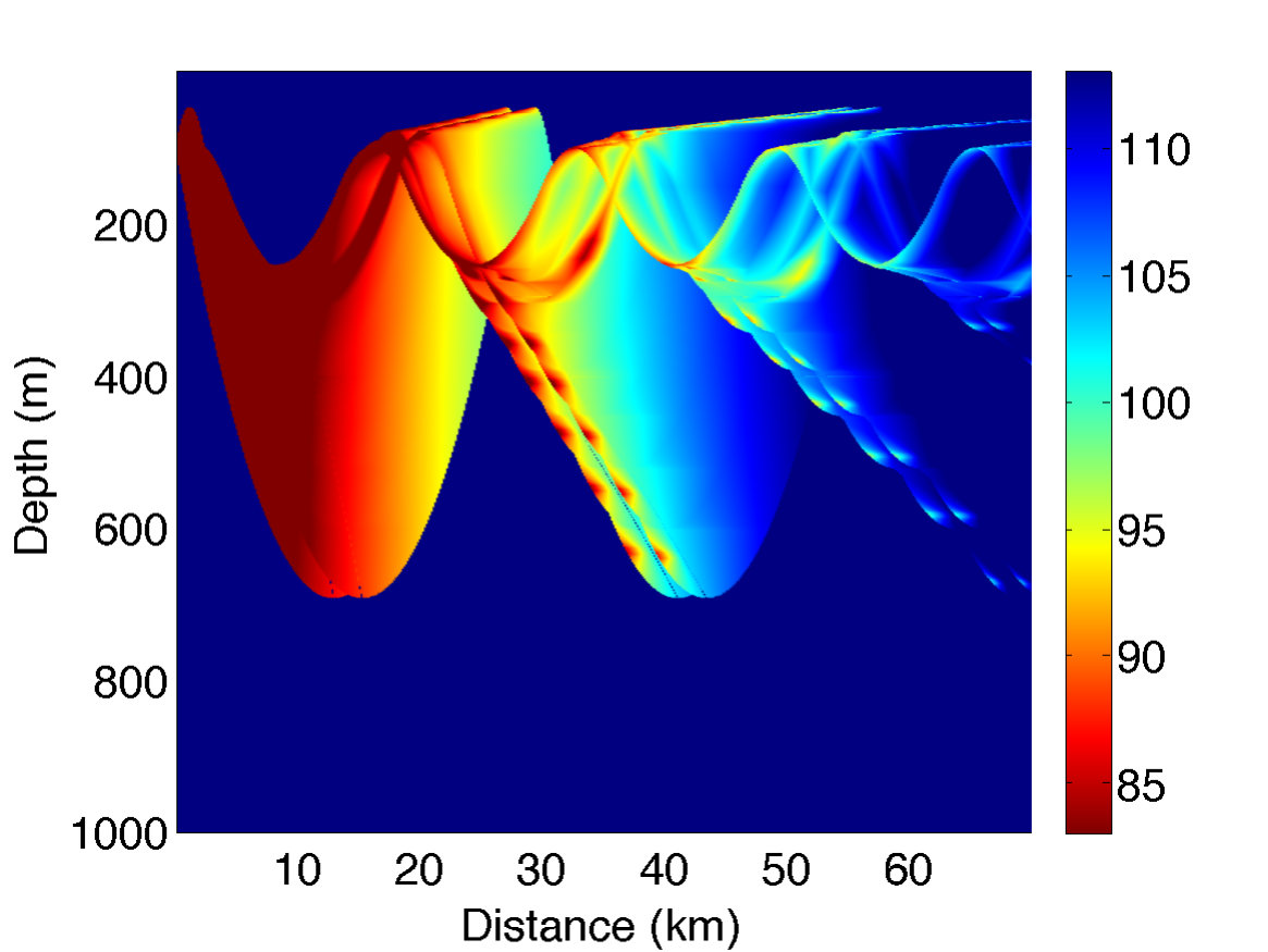 Figure 1
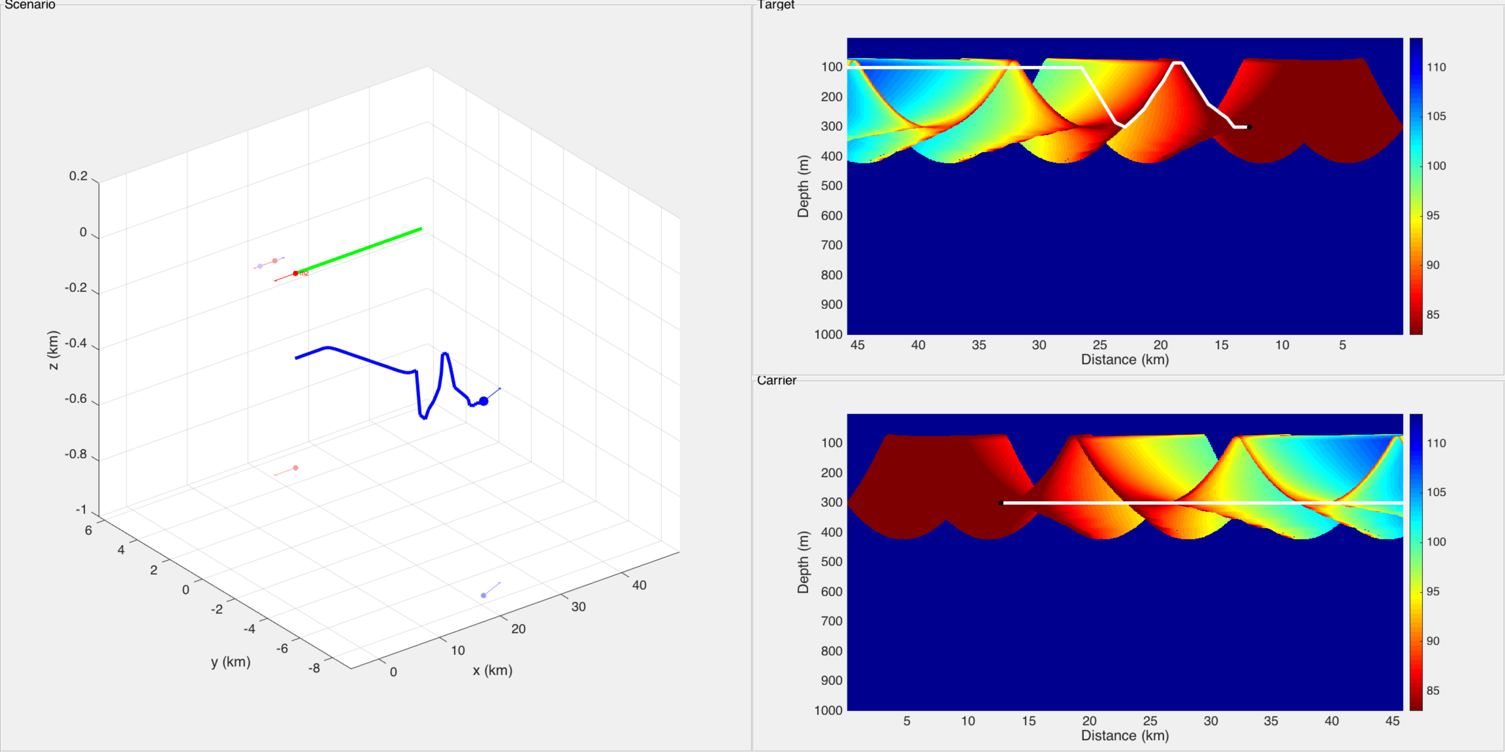 Figure 10
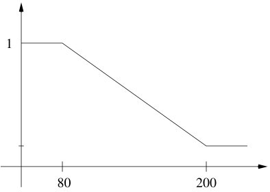 Figure 11
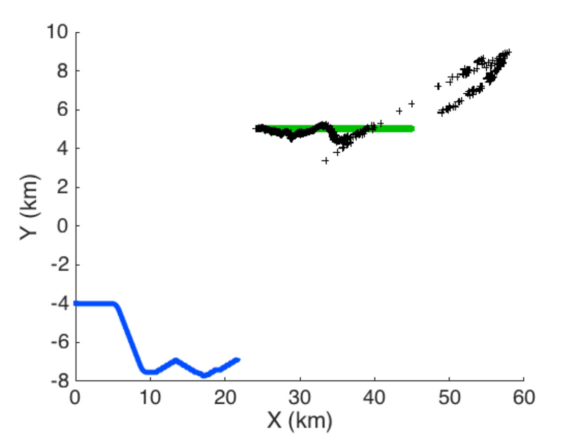 Figure 12
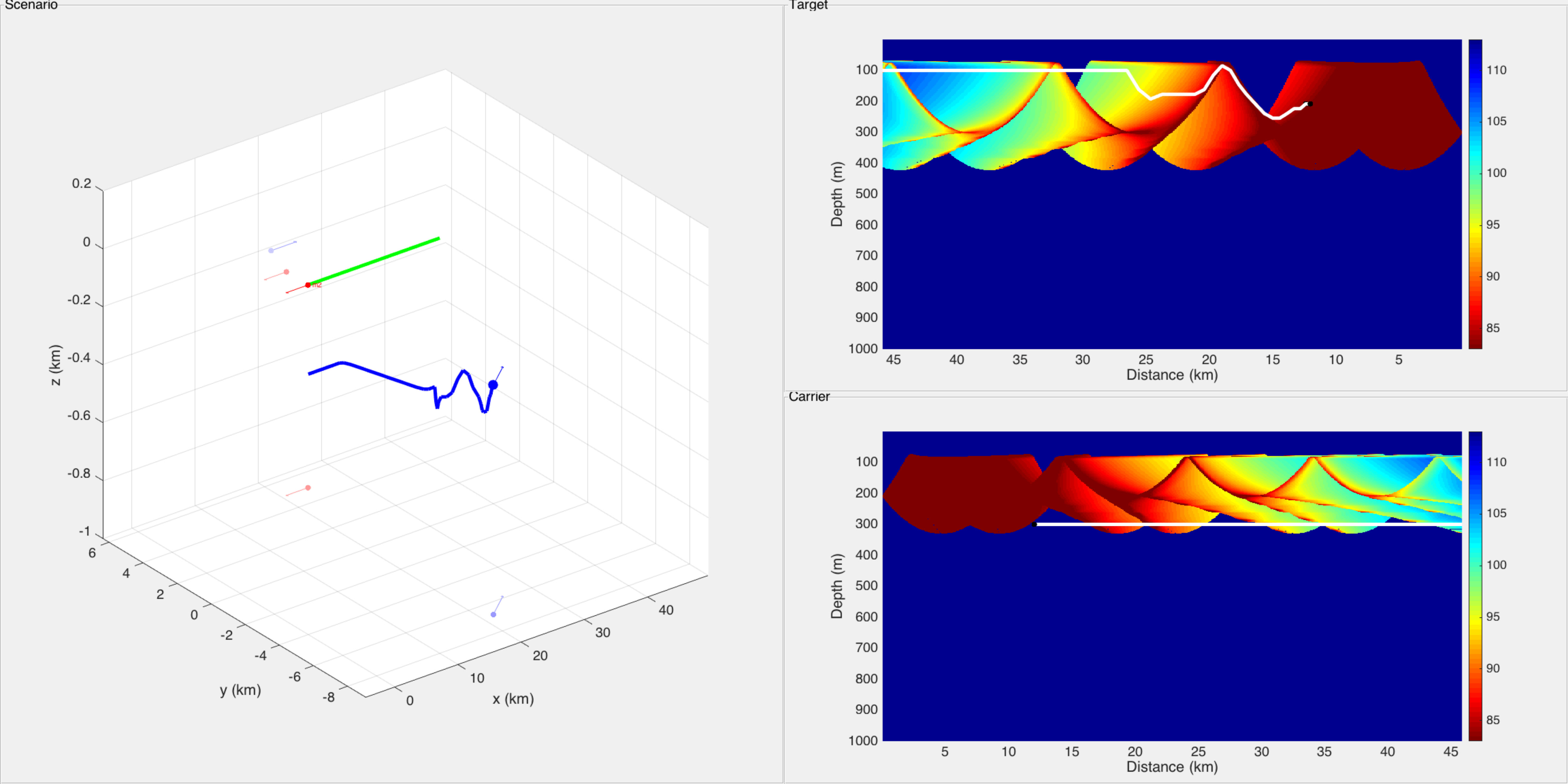 Figure 13
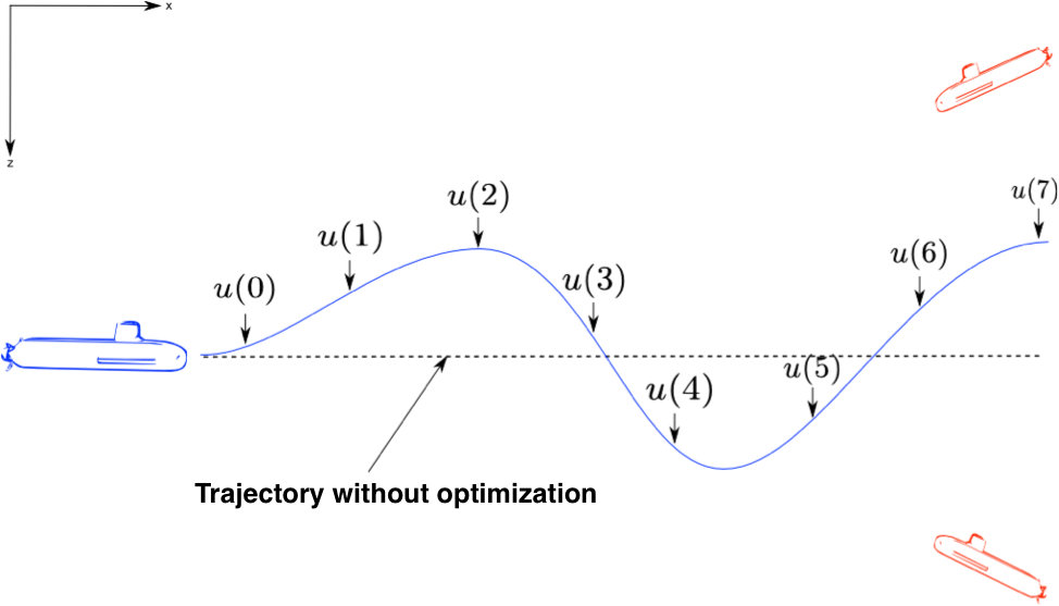 Figure 2
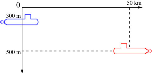 Figure 3
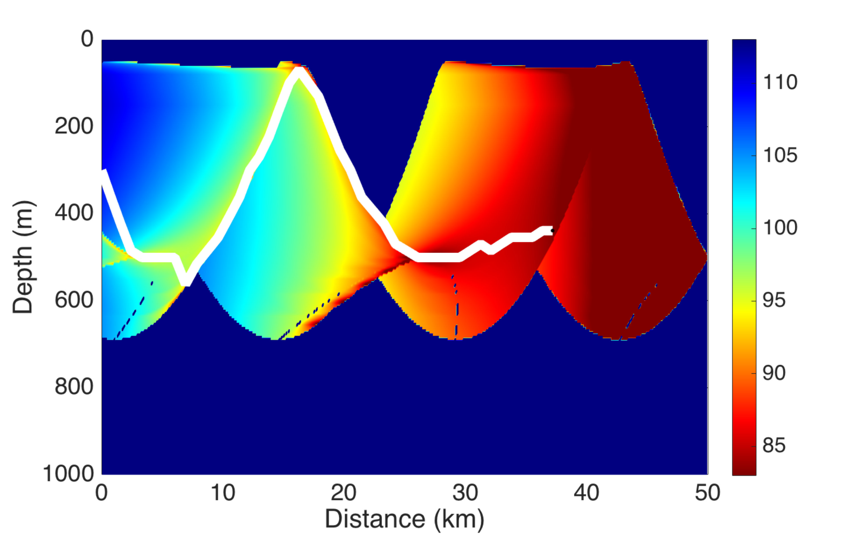 Figure 4
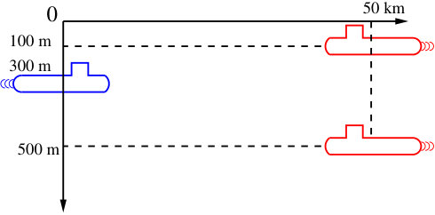 Figure 5
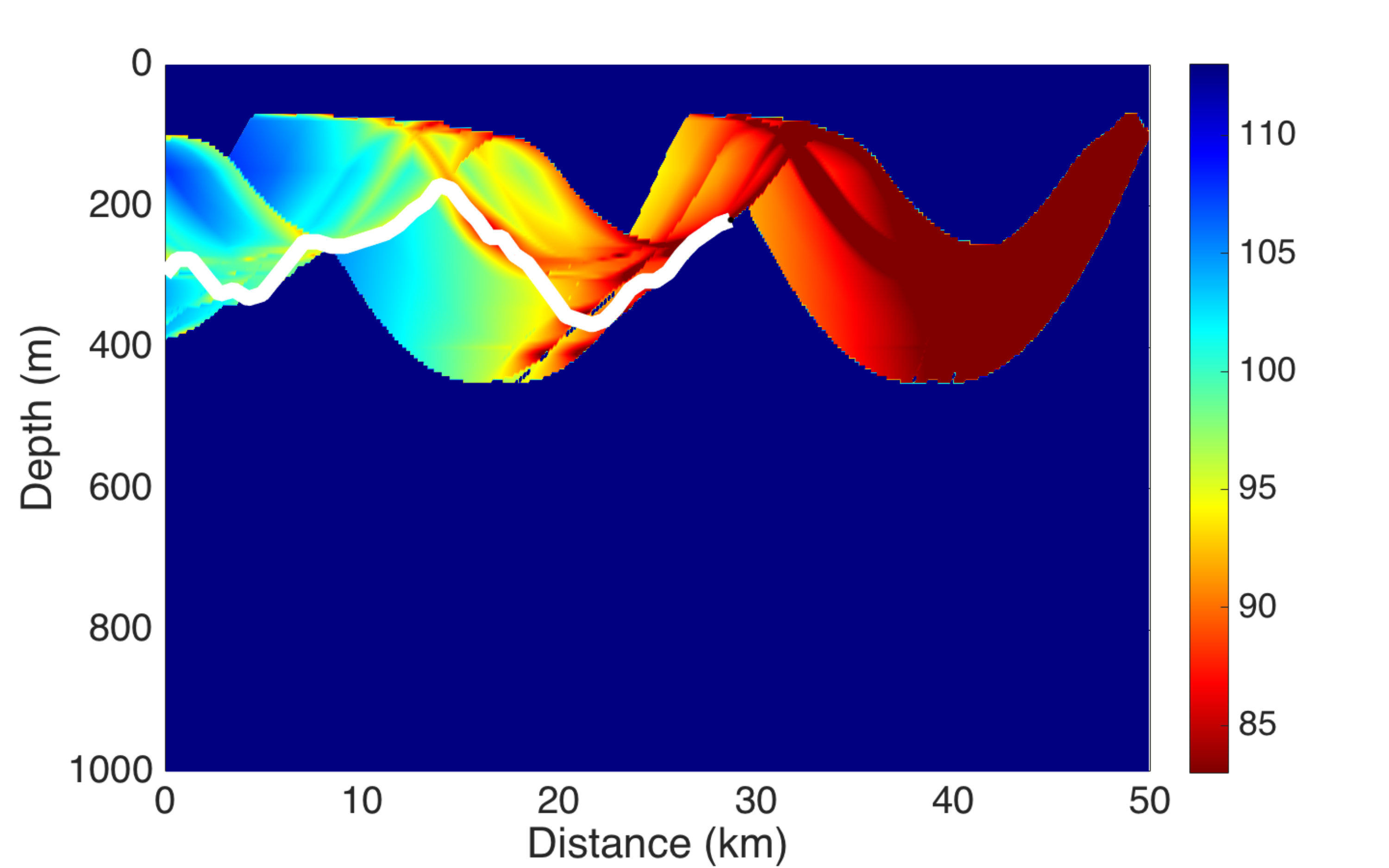 Figure 6
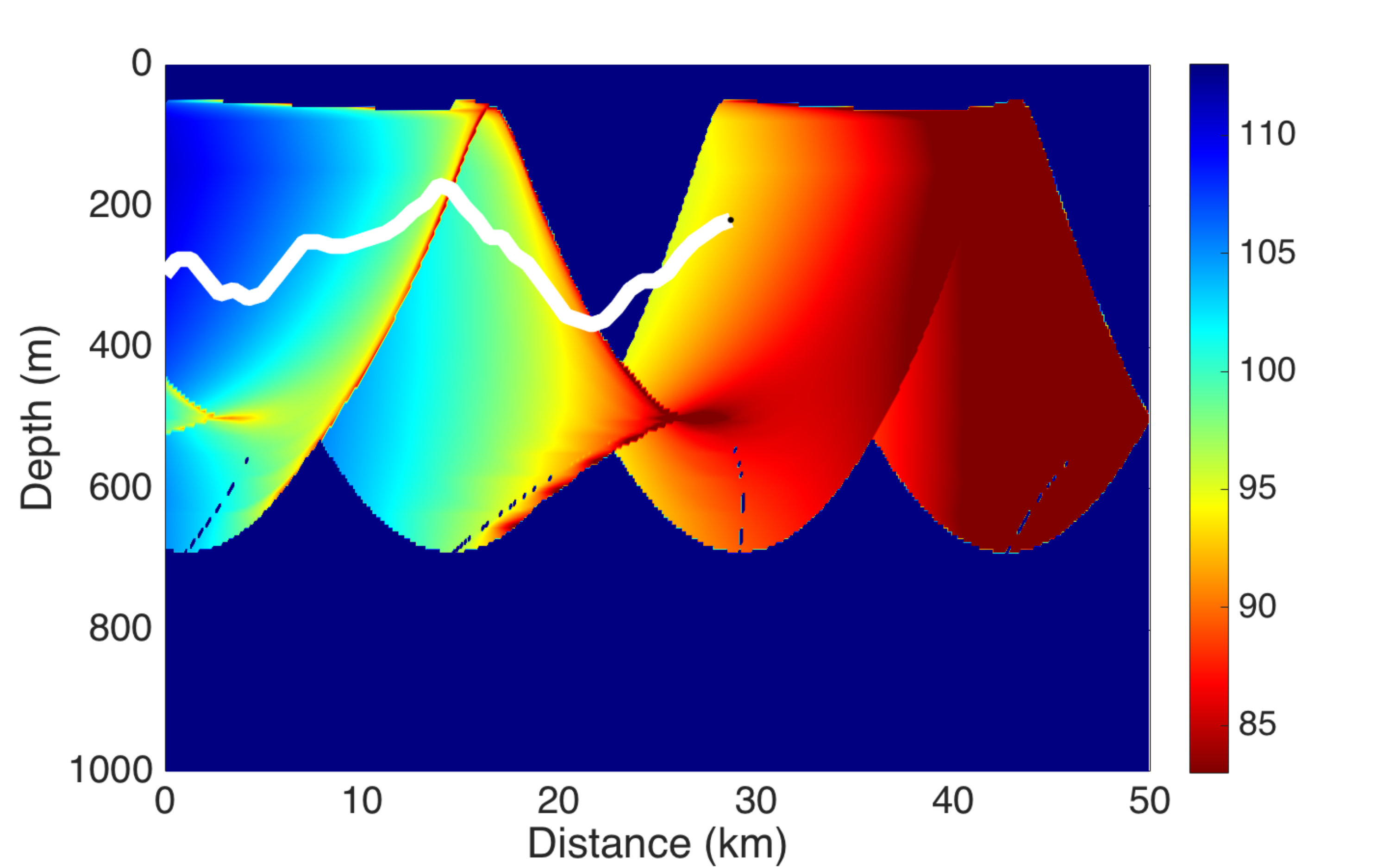 Figure 7
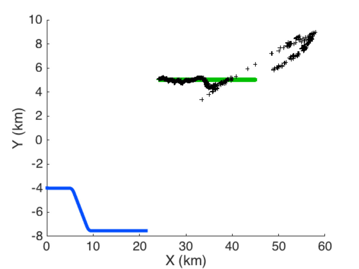 Figure 8
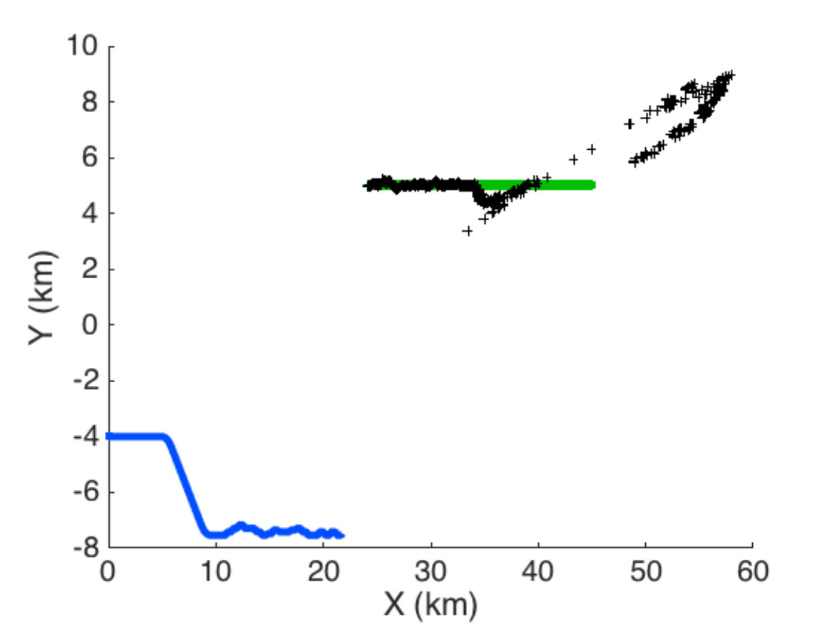 Figure 9
Peer Reviews
No public reviews on file for this paper yet. If you reviewed it on a platform where reviews are public (OpenReview, ICLR, NeurIPS, ICML), you can paste yours below so the community can read it here.
Videos
No videos yet. Explain this paper in a talk, walkthrough, or lecture? Add one.
Taxonomy
TopicsTarget Tracking and Data Fusion in Sensor Networks · Advanced Control Systems Optimization · Control Systems and Identification
Quantization and Stochastic Control of Trajectories of Underwater Vehicle in
Bearings-only Tracking
Huilong Zhang
Dann Laneuville
Univ. Bordeaux
CNRS IMB, UMR 5251
INRIA Bordeaux-Sud Ouest, France
DCNS Research
Nantes, France
Benoîte de Saporta
Adrien Nègre
Univ. Montpellier
CNRS IMAG, UMR 5149
INRIA Bordeaux-Sud Ouest, France
DCNS Research
Toulon, France
François Dufour
Inst. Polytech. Bordeaux
CNRS IMB, UMR 5251
INRIA Bordeaux-Sud Ouest, France
Abstract
We present in this paper a numerical method which computes the optimal trajectory of a underwater vehicle subject to some mission objectives. The method is applied to a submarine whose goal is to best detect one or several targets, or/and to minimize its own detection range perceived by the other targets. The signal considered is acoustic propagation attenuation. Our approach is based on dynamic programming of a finite horizon Markov decision process. A quantization method is applied to fully discretize the problem and allows a numerically tractable solution. Different scenarios are considered. We suppose at first that the position and the velocity of the targets are known and in the second we suppose that they are unknown and estimated by a Kalman type filter in a context of bearings-only tracking.
Index Terms:
Non linear filtering, Quantization, Markov decision processes, Dynamic programming, Underwater acoustic warfare.
I Introduction
Target tracking, in particular submarine target tracking, which role is to determine the position and velocity of the target has been extensively studied in the past decade [1, 2, 3]. To our knowledge, there is little work [4] that focuses on computation of optimal trajectories of underwater vehicle based on signal attenuation due to acoustic propagation and taking into account the uncertainties on the target position and velocity. The original aspect of our approach is to propose a mathematical computational model to address this problem.
In a context of passive underwater acoustic warfare, we are interested in optimizing the trajectory of a submarine called carrier. The carrier is equipped with passive sonars. A question naturally arises: how should the carrier position itself to detect at best the acoustic signal issued by other vehicles called targets? Conversely, given that the targets are also equipped with sonars, how should the carrier position itself to keep its own detection range as low as possible with respect to those targets? These two objectives being seemingly contradictory, is it possible to take into account both of them simultaneously? A smart operator, if provided information about a single target position and velocity and a sound propagation code can find a good trajectory for either one of these single objectives. If the two criterions are considered simultaneously, or if several targets have to be taken into account, it is hardly possible for a human operator to find the best route. Some decision making tools have to be developed to this aim.
One of the candidates are Markov decision processes (MDPs) which are widely used in many fields such as engineering, computer science, operation research. They constitute a general family of controlled stochastic processes suitable for modeling sequential decision-making problems under uncertainty. A significant list of references on discrete-time MDPs may be found in the survey [5] and the books [6, 7, 8, 9, 10]. The objective of this paper is to use this framework to compute optimal trajectories for underwater vehicles evolving in a given environment to meet some objectives such as mentioned above. In our preliminary works [4] and [11] we have applied this method to control a carrier whose mission was to detect one or several targets as well as possible. In [4] one important assumption was that the positions of the targets followed a random model but were perfectly observed at the decision dates. This assumption is unrealistic as the targets positions are usually only known up to some random error through sonar measurements. The assumption is abandoned in [11]. In the present paper we propose a control strategy for a carrier submarine in a context of bearings-only tracking (BOT).
It is well known that many real-world problems modeled by MDPs have finite but huge state and/or action spaces, leading to the well-known curse of dimensionality, which makes the solution of the resulting models numerically intractable. Our initial optimization procedure includes an optimized dynamic discretization of the space of the targets positions at each time step from the current time to the computation horizon. Adding uncertainty on the targets makes the space of the targets positions significantly larger. More points are thus required in the discretization grids to keep a satisfying accuracy, dramatically slowing down the global process: construction and optimization of the discretized grids, final trajectory optimization procedure. Simulation-based algorithms such as multi-stage adaptive sampling, evolutionary policy method and model reference adaptive search [10] can be used to overcome this difficulty. But in the context of BOT, these approaches can not be applied, since a filtering procedure has to be integrated. Under the consideration of practice, we choose to split the long-term horizon into a sequence of sub-intervals, making the global optimization sub-optimal but real-time achievable, as the discretization grids only need to be optimized on a shorter horizon.
Related works in the literature are for example model predictive control [12], moving horizon control [13] or receding horizon approach [14], where similar ideas of shortened horizon are used to make the problems numerically solvable in real-time. within the POMDP (partially observable Markov decision processes [15, 16]) framework, the most computationally tractable strategy is to use myopic open-loop feedback control. In [17], a sequence of shortened horizon H is fixed and Monte Carlo integration method is used to estimate reward fonction for each horizon.
Our focus is on computational approaches to find optimal policies. The paper is organized as follows. Section II states the problem in a general context and explains our strategy to solve it. Section III briefly outlines the dynamic programming algorithms used. Section IV presents the numerical results for four different scenarios, from the simplest case to the realistic case.
II Problem Statement
Underwater sound propagation in the sea depends on many environmental parameters such as temperature, salinity, etc. Indeed, small variations of these parameters may greatly modify the sound propagation (see for instance [18]). To illustrate this phenomena, Fig. 1 gives an example of a sound propagation diagram with an emitter source standing at a depth (top left). The signal loss level due to propagation usually takes values in . The emitter may well be detected by a carrier in the areas (distance to emitter versus depth of carrier) of lower signal loss level (, represented by dark red color), and a contrario is hardly detectable if not undetectable in higher signal loss level areas (, represented by dark blue color). Please also note that the carrier being close to the emitter does not guarantee a good detection. In this figure, the signal loss level is saturated to .
Let us consider a general situation with a carrier submarine of interest surrounded by one or several targets. This submarine carries passive sensors so that the available measurements are the estimated angles (bearings) from observer to sources. The trajectory of submarine has to be controlled in order to satisfy some given mission objectives. These can be e.g. optimizing the different targets detection range, minimizing its own detection range as perceived by the other targets, reaching a way-point with minimum fuel consumption, etc.
The following inputs are supposed to be available
perfect position and velocity, 2. 2.
noisy observation of the target, namely bearing and frequency, 3. 3.
information about the environment (sound speed, sea floor depth, bottom type, …).
A sound propagation code which calculates the signal loss level due to propagation (such as in Fig. 1) is also available.
The desired output is an optimized sequence of commands to pilot the carrier submarine in order fulfill its mission at best within a given time interval, see Fig 2.
Concerning the targets, their evolution is described by a stochastic model.
III Stochastic optimal control
As seen in Section II the problem is quite complex, there are uncertain inputs and a probabilistic modeling should be used to take account of this feature. A discrete stochastic optimal control framework seems to be a good candidate to solve this problem. More precisely, we use a discrete-time finite horizon dynamic programming approach. We first describe this approach for a single long-term optimization problem, then we will explain how to divide it into a sequence of short-term ones.
We have opted for the quantization technique to discretize the movement of the targets. As the targets evolve in an infinite continuous space, quantization offers both a discretized density and a transition matrix, required for MDP approach and allows for discretization grids that are dynamic and concentrated at the most probable positions of the targets. The aim is to compute an optimal trajectory by applying a command to ’s future states for all times up to the computation horizon, see Fig. 2.
In our framework, three probabilistic techniques are used, namely Kalman filter, quantization and dynamic programming, and each of these overlaps with one another and are combined in an iterative algorithm.
III-A Dynamic programming
In this section, we briefly introduce the discrete-time finite horizon Markov control framework. Let us consider the following model:
[TABLE]
with
- •
: finite space, namely the state space,
- •
: finite space representing the control or actions set,
- •
: family of non empty subsets of , being the set of feasible controls or actions when the system is in state . We suppose that is a measurable subset of ,
- •
: transition matrix on given which stands for the transition probability function,
[TABLE]
- •
: measurable function representing the cost per stage,
- •
: measurable function representing the terminal cost.
Suppose that a finite horizon and an initial state are given. The total expected cost of a policy ( is the set of all possible policies) is defined as
[TABLE]
The optimal total expected cost function is then defined as
[TABLE]
The goal is to find an optimal policy which optimizes this cost. The optimization criteria opt can be either inf (to minimize a loss) or sup (to maximize a performance) according to the mission’s type. The main idea of the dynamic programming principle is to recursively solve a sequence of one-step optimization problems by computing (backwards) a sequence of functions by the following algorithm
- •
,
- •
for and
[TABLE]
The last function thus constructed, , is the value function . In addition, the policy defined by with
[TABLE]
is an optimal policy, i.e. .
III-B Submarine
The movement of the carrier is assumed to be deterministic, modeled by the -dimensional vector for the carrier position at time . Its dynamic is determined by the control policy
[TABLE]
At each time step and at each position of sensor the control set is
[TABLE]
for some given space steps (related to the maneuverability of the carrier in the prescribed direction during the computation time step) and control ranges . The feasible controls at position are those that correspond to actual underwater positions (e.g. not above the sea level, not below the sea floor, not on shore, …). Therefore, we can consider that the submarine ’s state takes values at time in a -dimensional grid whose size increases gradually
[TABLE]
III-C Targets
The modeling of the targets being similar and independent of each other, we will consider only one target in this section. The multi-target case will be discussed in Section IV-B. We suppose that the target evolves with a constant depth and that its dynamics is independent of the carrier . The target kinematics are modelled using 2-dimensional Cartesian position and velocity vectors . Its evolution is described by the stochastic model
[TABLE]
where F=\left[\begin{array}[]{cc}1&T\\ 0&1\end{array}\right]\otimes I_{2},\leavevmode\nobreak\ \leavevmode\nobreak\ K=\left[\begin{array}[]{c}T^{2}/2\\ T\end{array}\right]\otimes I_{2}, , is a 2-dimensional independant noise with . The parameters are given a priori standard values.
Thus the natural state space for the target is continuous. However, to apply the dynamic programming approach described in part III-A, we need a finite state space. Hence, it is necessary to approximate the continuous state space with a finite one.
Various methods exist for this approximation [19]. We chose a quantization method as it is dynamic and suitable to discretize random processes. The goal of this method is to approximate the continuous state space Markov chain by a finite state space chain . To this aim we use the quantization algorithm described in [20, 21, 22]. Roughly speaking, more points are put in the areas of high density of the random variable. The quantization algorithm is based on Monte Carlo simulations combined with a stochastic gradient method. It provides grids, one for each (), with a fixed finite number of points in each grid. The algorithm also provides weights for the grid points and probability transition between two points of two consecutive grids, thus fully determining the distribution of the approximating sequence (). The quantization theory ensures that the distance between and tends to 0 as the number of points in the quantization grid tends to infinity [21]. In our case, the process is approximated by a finite Markov chain with the following notation
- •
is the quantization of and is the point grid at time ,
- •
is the transition matrix, , .
There exists extensive literature on quantization methods for random variables and processes [23, 24, 20, 21, 22, 25].
III-D Markov control model
We can now fully describe the Markov control model corresponding to our problem. The finite state space is , where . The process at time is . Component evolves deterministically while is stochastic. The action space is described in Section III-B.
The process is not controlled hence the transition matrix can be obtained from as
[TABLE]
for all and .
The transition cost function from state to state given a control is . In our application, this function only depends on the sound propagation code which is geometric (its values only depend on the submarine and target relative positions and some fixed parameters). Hence . We finally obtain the following dynamic programming equation
[TABLE]
III-E Algorithm
In the case where the position and velocity of the target are known, the resolution of our stochastic optimal control problem can be divided in three steps. The first step is an optimal quantization in order to approximate the target state by a finite Markov chain state. The second step is a backward dynamic programming algorithm for evaluating the best policy from each possible system state. This step only depends on the law of the process. The last step is on line, it consists in applying the optimal control policy to a given trajectory of the process.
The case where the state of the target is unknown is described in IV-C and IV-D.
Step 1: Quantization
The goal is to approximate by a finite Markov chain . Algorithm 1 describes how to adapt the CLVQ (competitive learning vector quantization) technique to the context of an optimal quantization of a Markov chain. We refer the reader to [26, section 3.3] for the computation of the weights and transition matrices by Monte Carlo simulations.
We obtain for each time a grid and the corresponding transition matrix . Grid and transition matrices are stored. Let be the optimal -quantization of the random variable for by a random variable taking points. Let us denote by the grid at step and the associated Voronoi tessellation . Clearly, the process is not a Markov chain. However, at each step one can compute
[TABLE]
for . The marginal quantization approximation of the Markov chain is then defined by the Markov chain whose transition matrix at step is given by \big{(}\hat{P}^{t}_{i,j}\big{)}_{0\leq t\leq N-1}, and the initial distribution of is given by that of . It can be shown (see for all the details [21, Theorem 3.1]) that the joint distribution of can be approximated by that of with a rate of convergence of order , where is the dimension of the state space.
Step 2: Pre-computations
Compute for each possible state element
[TABLE]
the optimal control policy that optimizes the cost function for horizon .
Step 3: On line selection of optimal action
As we suppose that the trajectory of the target is known, the selection of the optimal action given the current state and time (see algorithm 4) can be done on line.
IV Numerical results
In order to illustrate numerical results, several scenarios with different mission objectives have been considered.
Scenario 1 : one target, its state (position and velocity) is known, objective is to detect at best the acoustic signal issued by the target. 2. 2.
Scenario 2 : two targets, their states are known, objective is to detect at best the acoustic signal issued by the two target. 3. 3.
Scenario 3 : one target, its state is unknown, objective is to detect at best the acoustic signal issued by the target. 4. 4.
Scenario 4 : one target, its state is unknown, objective is to detect at best the acoustic signal issued by the target and at same time to keep its own detection as low as possible.
The first scenario allows to validate the algorithms presented in Section III-E. A special technique of quantization is proposed for the multi-target scenario. The third and fourth scenarios are more realistic, we will split the time horizon into subintervals to make the computation feasible.
IV-A Scenario 1
We consider here the simplest scenario : there is a single target in the environment. The carrier wants to best detect the target. The initial geometry is depicted by Fig. 3. The target (red) follows a uniform motion and its depth remains constant (500 m). At initial time the depth of the carrier submarine is 300 m. The relative target-carrier speed is 10 .
In this scenario we assume that the position of target is known at the decision time, and at each time step, available controls are in one dimension (), which means that the only control action is change of depth. Results are illustrated in Fig 4. The diagram represents the sound propagation loss of target, and the trajectory of carrier is plotted by white dot points. We can see that the movement of carrier is “intelligent” in the sense that its position is always in the red aera, where the sound acoustic loss of target is lower.
IV-B Scenario 2
Let us consider a more complex scenario with two targets at different depth. The first target is at 500 m depth whereas the second target has a depth of 100 m (see Fig. 5). In this scenario, the available controls are also in one dimension.
In the case of multi-target, there are two ways to quantify the movement of targets. The first ways is to quantify each target separately and independently, because the evolution of the targets is assumed to be independent. The second method is to regroup the targets in one state space by increasing the dimension of state space. For this scenario we can quantify the movement of two targets ( and ) by model
[TABLE]
This choice is justified by following considerations : the first method of quantization is numerically intractable, since two quantization grids ( and ) will be necessary and the cardinal of the set is too great to be numerically feasible. Using the second quantization method, some numerical dependence will be introduced and dimension of model (7) is twice that of the previous example. Let be the quantization of quantization at time calculated by model (7). Then a point of represents a couple . Let’s denote by
- •
a quantization point à time
- •
the transition matrix
[TABLE]
So the dynamic programming equation (6) remains unchanged.
The multi-target cost function is defined in order to keep a good detection range of each target. Let be the position of carrier, the position of targets 1 and 2, and acoustic loss value of targets 1 and 2 regarding the carrier, then the cost function can be calculated by
[TABLE]
We take . The coefficients and can be modified if we privilege the detection one of two targets.
Fig. 6 and Fig. 7 illustrate the sound propagation loss diagram of targets 1 et 2 respectively, and the trajectory of carrier is plotted by white dot points. We can see that the movement of carrier is also “intelligent” in the sense that for most of the time, it is positioned in “good” area, where the acoustic loss is lower for both targets. But during certain periods, it is physically impossible to stay simultaneously in red areas for both targets. For instance in Fig. 7 when the distance with target is at 20 km, it is impossible to maintain the carrier in the reddish area of the two targets. However note that the carrier never reaches the blue area of both targets simultaneously.
IV-C Scenario 3
In the last two scenarios we consider that the position and velocity of target are unknown. This assumption is more realistic because the targets positions are usually only known up to some random error through sonar measurements. In this article we propose a control strategy for a carrier submarine in a context of bearings-only tracking (BOT).
It is well known that when the target and carrier are under uniform rectilinear motion, the filter of BOT does not converge because the problem is not obervable, some maneuvers have to be performed by the carrier in order to get a precise enough approximation. Therefore we divide our operations into two periods. In the first period there is no control, only the target motion analysis (TMA) filter algorithm is run. In the second period both filter and control algorithms are run, the latter being fed by the former.
In scenario 1 and 2, a long optimization time horizon is performed. Unfortunately, these pre-computations are strongly dependent on the estimated initial position of the targets. Therefore, there is no hope of being able to run it in real time taking into account the regularly updated outputs from the TMA algorithm. In order to circumvent this difficulty, we chose to divide the originally long-term optimization problem into a sequence of short-term ones. This procedure is of course sub-optimal, but it is compatible with real time applications and it gives fairly good results.
Horizon splitting technique
To solve numerically the dynamic programming equations of a finite horizon Markov decision process, the parameter horizon is decisive from the computation time and memory consumption points of view. Indeed, we need to calculate a priori the optimal control associated with each quantization grid point for each time step. In addition one needs to build and optimize the quantization grids which get larger as the time horizon increases.
In terms of memory, we need to store the transition matrices of size , where is the number of points in the grids . In terms of complexity of the algorithm, the computation time increases geometrically with , because the size of the control space increases geometrically. Unlike scenario 1 and 2 where the available controls are in one dimension, we suppose that the control space is in three dimensions , therefore a long horizon will lead to an unsolvable problem. In addition, we have to calculate the sound propagation diagram (i.e. cost function in algorithm 2) for each control point.
To make the computations tractable, we propose a splitting technique: we divide the long-term horizon into subintervals, and we build the short-term quantization grids once for each subinterval and apply the short-term dynamic programming algorithm on each subinterval, in an iterative manner. Although this is sub-optimal compared the original long-term horizon problem, it greatly shortens the computation time and makes it possible to run our procedure on line.
At each time step , two calculations are performed successively as follows. First, the TMA process with an Unscented Kalman filter (UKF) is performed to estimate the actual position of the target at time . Then one selects the best action given the carrier and target current positions. Suppose that is beginning time of sub-optimal interval, is end time of subinterval, and the state of the target at time is estimated by a probability distribution , which is the output of the UKF filter at end time of precedent sub-optimal interval. This distribution is used as initial condition to start quantization. Algorithm 2 is applied to pre-calculate optimal control for every quantization point. As the position and velocity of the target are unknown, (only their estimations are available), we then search in the cloud of quantization grid points the point that is closest to the filtered position and the optimal control corresponding to this grid point is applied at this time step. Algorithm LABEL:algo2_controle_optimale_en_ligne is a amended version of algorithm 4.
A consequence of the horizon splitting technique is that the quantization grid is automatically updated at the beginning of every subinterval. A quantization grid can be considered as an approximation of the conditional density given the observations. When the UKF filter has converged, the grid points are more concentrated, then accuracy of the MDP calculation increases.
In this scenario there are one carrier submarine and one single target in the environment. Objective of the carrier submarine is to detect at best the target. The scenario lasts 45 min. The target follows a rectilinear motion, and its depth remains constant (300 m). Its position is represented by the green curve in Figs. 8, 9 and 12, and the green curve in Figs. 10 and 13. At each time step, the sensor of the carrier submarine processes two measurements (bearing and frequency). Though in this case the problem is known to be observable, the performance of the filter is quite poor if no maneuvers are scheduled. In our scenario, two maneuvers are planned. The first maneuver is a right turn at t = 10 min, which lasts 2 minutes, the second is a left turn at t = 20 min, which also lasts 2 minutes. These maneuvers allow the filter to converge, thereafter the submarine follows a rectilinear motion if no control is applied. Fig. 8 illustrates the scenario in the horizontal plane without stochastic optimal control (without the depth coordinate as both carrier and target remain at constant depth). The trajectory of the carrier submarine is represented by the blue curve (starting from the left), the real trajectory of the target by the green line (starting from the right) and the black curve represents the TMA filter’s estimated position of the target.
In order to have an accurate enough estimation of the target position, we have divided this scenario into two periods (the time step being minute).
- •
Filtering-only period (0-22 min). In the first period, only the TMA filter is enabled, the period expires at the end of the two maneuvers.
- •
Filtering and optimization period (22-45 min). This period begins immediately after the first period, The three steps algorithms presented in Section III-E are applied times for a -minute horizon optimization.
The numerical results show that when the estimation of the target position is of poor quality (error and standard deviation too large), efficient control of the trajectory of the submarine is impossible.
As in scenario 1, the cost function is only based on the sound diagram emitted by the target. The numerical results are illustrated by two figures. Fig. 9 shows the result of filtering. Only the horizontal plane (X-Y) without depth is illustrated. Fig. 10 shows the signal loss due to sound propagation emitted by the target (above) and by the carrier submarine (below), the trajectories in 3D are shown in the left (green: target, blue: carrier). The white curve in this diagrams stand respectively for the carrier depth and for the target depth. Note that
- •
from min, the trajectory of the carrier submarine is very different compared to the original scenario where there is no control (see Fig. 8 for comparison). It was modified by the dynamic programming procedure, and the quality of the TMA filter is not degraded;
- •
the target diagram signal loss shows that the dynamic programming has well performed as a controller because, in the second period, the carrier submarine remains in the zone of high detection level (reddish zone), despite the fact that we replaced the true position of the target by its filtered estimation;
- •
the carrier diagram signal loss is also presented in Fig 10, but it does not reflect the reality of the past trajectory, because the submarine depth was changed after min leading to a change of its diagram. As the diagram is changing over time, we cannot represent it on a static figure. See the web site [27] for a video version. It can be seen that the carrier submarine can sometimes be easily detected by the target because the carrier submarine sound propagation diagram was not taken into account in this scenario.
IV-D Scenario 4
We now take fully into account the original mission where two seemingly contradictory objectives are to be achieved. The first objective is to pilot the sensor so as to detect at best the acoustic signal issued by the target, the second objective is to keep its own detection range as low as possible. In this case, the objective function is a multi criteria aggregation function whose optimization will be a trade-off between the conflicting objectives. We will take into account the diagrams emitted by the carrier submarine and the target simultaneously in our approach.
Compared to scenario 3, we use the same scenario parameters, the only modification is the cost function used in equation (6). Instead of using a weighted sum as in the problem of multi-target (8), we apply the following method. Let be the position of the carrier submarine, that of the target, (resp. , the value extracted from the sound propagation diagrams emitted by the target (resp. by the carrier submarine). These values vary in the interval . The objective of the mission is to place the submarine in the area where the value of is as low as possible and the value of as high as possible. Then the cost function associated to is defined by
[TABLE]
where is the following function
[TABLE]
where and are chosen to satisfy the continuity conditions: and . Fig. 11 illustrates the function.
The optimization problem is a minimization of the cost function. The range of varies in interval . When it is in the area where the multiplier is 1, penalizing this area; when the multiplier is making this area of lower cost. In between, is a linear function. Thus we penalize the area where is near 80 without excluding them completely.
The numerical result are presented in Figs. 12 and 13. The trajectory of the carrier submarine is different from that of Figs. 9 and 10, because the cost function and the control policy are different. Fig. 13 shows the target and carrier signal loss diagrams respectively. Note that the detection of the target by the carrier submarine is of lower quality than before, in the sense that the carrier submarine is not always in the area of darkest red color. However, the diagram of the carrier submarine is now much more interesting: with a few exceptions, the target remains in the blue area, which means that the carrier submarine is undetectable by the target. See the video version of this result [27] for details. This numerical example shows that the two objectives can be realized.
V Conclusion
In this paper we have proposed an original and effective control strategy for sensor management in a context of uncertainty of the targets positions. Four scenarios are considered, from simple academic case to realistic case. We showed that it is possible to plan a sensor trajectory even for possibly conflicting objectives. With partition technique, the execution time is significantly reduced and the approach can be performed in real time. Although this partition method is sub-optimal, it gives very satisfactory results, keeping the carrier submarine position in the desired areas.
The reference list from the paper itself. Each links out to its DOI / PubMed record.
- 1[1] B. RISTIC, S. ARULAMPALAM, and N. GORDON, Beyond the Kalman Filter : Particle Filters for Tracking Applications . Artech House, 2004.
- 2[2] D. LANEUVILLE and C. JAUFFRET, “Recursive bearings-only TMA via unscented kalman filter : Cartesian vs. modified polar coordinates,” in Proceedings Aerospace Conference , (Big Sky, MT), IEEE, March 2008.
- 3[3] E. BASER and I. BILIK, “Modified unscented particle filter using variance reduction factor,” in Proceedings of the 2010 IEEE Radar Conference , IEEE, May 2010.
- 4[4] A. NEGRE, O. MARCEAU, D. LANEUVILLE, H. ZHANG, B. de SAPORTA, and F. DUFOUR, “Stochastic control for underwater optimal trajectories,” in Proceedings of the 33th IEEE Aerospace conference , IEEE, Mar. 2012.
- 5[5] A. ARAPOSTATHIS, V. S. BORKAR, E. FERNANDEZ-GAUCHERAND, M. K. GHOSH, and S. MARCUS, “Discrete-time controlled markov processes with average cost criterion: a survey,” SIAM Journal on Control and Optimization , vol. 31, no. 2, pp. 282–344, 1993.
- 6[6] D. P. BERTSEKAS and S. SHREVE, Stochastic optimal control : the discrete time case . Volume 139 of Mathematics in Science and Engineering, New York: Academic Press Inc., 1978.
- 7[7] O. HERNANDEZ-LERMA and J. LASSERRE, Discrete-time Markov control processes , vol. 30 of Applications of mathematics . New York: Springer-Verlag, 1996.
- 8[8] O. HERNANDEZ-LERMA and J. LASSERRE, Further topics on discrete-time Markov control processes , vol. 42 of Applications of mathematics . New York: Springer-Verlag, 1999.