On the image of the parabolic Hitchin map
David Baraglia, Masoud Kamgarpour

TL;DR
This paper characterizes the image of the parabolic Hitchin map across classical groups and G2, revealing it is generally affine space, with exceptions for certain 'bad' parabolics in type D where singularities occur.
Contribution
It provides a comprehensive determination of the Hitchin map's image for all parabolics in classical groups and G2, highlighting cases with singularities.
Findings
Image is affine space for all parabolics except specific type D cases.
Identifies 'bad parabolics' where the image can be singular.
Provides explicit descriptions of the Hitchin map's image.
Abstract
We determine the image of the (strongly) parabolic Hitchin map for all parabolics in classical groups and . Surprisingly, we find that the image is isomorphic to an affine space in all cases, except for certain "bad parabolics" in type , where the image can be singular.
Click any figure to enlarge with its caption.
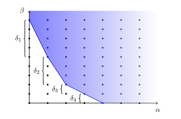 Figure 1
Peer Reviews
No public reviews on file for this paper yet. If you reviewed it on a platform where reviews are public (OpenReview, ICLR, NeurIPS, ICML), you can paste yours below so the community can read it here.
Videos
No videos yet. Explain this paper in a talk, walkthrough, or lecture? Add one.
\DefineSimpleKey
bibmyurl
On the image of the parabolic Hitchin map
David Baraglia
and
Masoud Kamgarpour
Department of Mathematics, University of Adelaide
School of Mathematics and Physics, The University of Queensland
Abstract.
We determine the image of the (strongly) parabolic Hitchin map for all parabolics in classical groups and . Surprisingly, we find that the image is isomorphic to an affine space in all cases, except for certain “bad parabolics” in type , where the image can be singular.
2010 Mathematics Subject Classification:
17B67, 17B69, 22E50, 20G25
Contents
- 1 Introduction
- 2 Proof of Theorem 7 for Type A
- 3 Local results for Types , , , and
- 4 Local results for Type
- 5 Proof of the main global results
- 6 Completion of the proof of the main local results
1. Introduction
The Hitchin map on the moduli space of Higgs bundles [Hitchin1, Hitchin] lies at the crossroad of geometry, Lie theory, and mathematical physics. It has found remarkable applications in non-abelian Hodge theory [Simpson90, Simpson] and the Langlands program [BD, Ngo]. The original construction of Hitchin was on compact Riemann surfaces. The generalisation to non-compact surfaces has been developed in, e.g., [SimpsonNonCompact, Boalch, BKV]. The relevant objects in the non-compact case are parabolic Higgs bundles.111To be more precise, one should consider parahoric Higgs bundles; cf. [BKV]. In this text, however, we restrict ourselves to the parabolic case. The aim of this paper is to determine the image of the Hitchin map on the moduli space of parabolic Higgs bundles. We start by stating a “local version” of our result, since this can be formulated in standard Lie-theoretic language.
1.1. Main local result
Let be a simple simply connected algebraic group over and let denote its Lie algebra. According to a theorem of Chevalley, the invariant ring is isomorphic to a graded polynomial ring with homogenous generators . These generators are not canonical; however, their degrees are, up to re-ordering, canonical invariants of called the fundamental degrees.
Let denote the local ring of formal power series over in the variable and let denote the quotient field of . Consider the map
[TABLE]
Here, is the -dimensional affine space over . We are interested in determining the image of certain subspaces of under this map. These subspaces are closely related to parabolic subalgebras of . Let be a parabolic subalgebra, and let denote its Levi decomposition. Let
[TABLE]
One of our main goals is to describe explicitly.
Remark 1*.*
The map is a local analogue of the Hitchin map on the moduli space of Higgs bundles. As we explain below, the space may be interpreted as the space of germs of (strongly) parabolic Higgs fields around a marked point with parabolic structure. Thus, is a local analogue of the image of the parabolic Hitchin map. This is our motivation for studying . Our notation is motivated by the fact that is a parahoric subalgebra of and is its annihilator under the canonical non-degenerate pairing on ; cf. [BKV].
Remark 2*.*
To make the above problem more tractable, we consider the closure of in . Let us explain what we mean by the word “closure” here. In fact, it is easy to see that takes values in for some positive integer . Now we think of as a pro-algebraic variety over
[TABLE]
where . By definition, a subset is dense if and only if is dense in the Zariski topology for all .
Notation 3*.*
Let denote the closure of in .222It may be that is closed in , but we do not know how to prove this, except in Type .
To give a description of , we will fix a specific basis of invariant polynomials in the following way:
Assumption 4*.*
If is an matrix, we write
[TABLE]
We use the following generators for the invariant ring:
- •
Type : identify with traceless matrices and use as generators.
- •
Type : identify with skew-symmetric matrices and use .
- •
Type : identify with matrices preserving a symplectic form and use .
- •
Type : identify with skew-symmetric matrices and use . Here denotes the Pfaffian, which satisfies .
- •
Type : take the embedding and use ; cf. [HitchinG2, §5.2].
Remark 5*.*
Note that in all cases except type , our chosen invariant polynomials are ordered by degree. However, in type , we do not order our invariant polynomials by degree. This convention is required for the statement of Theorem 7.
It turns out that admits a simple description in most cases under consideration. However, for certain parabolics subgroups in type , the structure of is considerably more complicated. In the introduction, we shall only give the description of in the “good” cases; i.e., those which satisfy Assumption 6 below. The precise description of in the “bad” cases is left to §4.
Assumption 6*.*
Assume that the pair is one of the following types:
- (1)
is of type , , , or and is arbitrary, or, 2. (2)
is of type and is the parabolic subalgebra of corresponding to a subset of simple roots, with satisfying , where the simple roots of are as indicated in the following diagram:
\alpha_{1}$$\alpha_{2}$$\alpha_{n-2}$$\alpha_{n-1}$$\alpha_{n}
To understand this condition better, set and . Then the Levi of has the form:
[TABLE]
and our assumption says .
Let denote the fundamental degrees of the Levi subalgebra . Note that as is not semisimple, it will have as a fundamental invariant (possibly with multiplicity). Now we have:
Theorem 7**.**
Under Assumptions 4 and 6, we have
[TABLE]
Remark 8*.*
In this theorem, we always put the fundamental invariants of in increasing order , but the fundamental invariants of are not necessarily in increasing order if is of type , see Remark 5.
This theorem can be considered as a refinement of a part of [Zhu, prop. 3.10].333A quantum analogue of Zhu’s result appeared in [CK]. We prove the inclusion of Theorem 7 by a direct computation. These computations are similar to the ones in [KL, §9]; see also [Rohith] for an alternative approach in Type . In Type , we prove the inclusion of Theorem 7 by constructing an appropriate companion matrix. We do not know how to construct these companion matrices in other types. Thus, to establish the inclusion beyond Type , we have to resort to global methods (see below).
Example 9*.*
Suppose and let
[TABLE]
Here, we have , , and , , . An explicit computation shows that in agreement with the above theorem.
Remark 10*.*
Let us explain the necessity of using the coefficients of characteristic polynomials. Indeed, in the example above, it is easy to see that there exists such that has a pole of order . Thus, Theorem 7 does not hold if we use traces of powers of matrices as algebraically independent generators for the invariant ring of .
Remark 11*.*
Consider a parabolic in Type that does not satisfy Assumption 6. As shown in §4, in this case, has a complicated description, regardless of what basis of invariant polynomials we choose. In fact, we show that the global analogue of (denoted by below) can be singular for these parabolics. This is in sharp contrast with the fact that when the assumptions are satisfied, is isomorphic to an affine space (Theorem 17).
Remark 12*.*
In [GW], Gukov and Witten call the image of the parabolic Hitchin map, the fingerprint of surface operators and identify it as one of the key ingredients for checking Langlands duality of Hitchin fibres. In §4 of op. cit., they conjecture that it should be possible to describe the image of the parabolic Hitchin map using the Kazhdan-Lusztig map from nilpotent orbits to conjugacy classes in the Weyl group [KL, §9]. Unfortunately, we were not able to make this conjecture precise.
1.2. Main global result
Let be a smooth projective curve over of genus and let denote the canonical bundle on . Let , , be parabolic subgroups of . Let , , be marked points on . A parabolic -bundle of type is a -bundle on equipped with -reduction of at ; cf. [LS]. Here, denotes the restriction of to .
Notation 13*.*
In what follows, for the ease of notation, we assume that we have only one marked point and one parabolic . The generalisation to finitely many parabolics introduces no additional complications. We let denote the moduli stack of parabolic -bundles on of type .
A (strongly) parabolic -Higgs bundle of type is a parabolic -bundle of type together with a section whose residue at lies in the nilpotent radical . We let denote the moduli stack of parabolic -Higgs bundles on of type . Observe that, with respect to a local trivialisation of and of around , the germ of at is given by an element of . It is in this sense that corresponds to local parabolic Higgs fields.
Example 14*.*
If , then a -bundle is the same as a rank vector bundle and a parabolic -bundle (of type ) is a pair consisting of a vector bundle of rank and a flag of subspaces of
[TABLE]
such that the stabiliser of this flag is . A parabolic -Higgs bundle of type consists of a vector bundle and flag as above, together with a section such that the residue of at maps to .
Definition 15**.**
The Hitchin map on is defined by
[TABLE]
Notation 16*.*
Let denote the Zariski closure of the image of .
The finite dimensional affine variety can be considered as the global analogue of , introduced in §1.1. As in the local setting, we prove that admits a simple description in most cases under consideration:
Theorem 17**.**
Under Assumptions 4 and 6, we have
[TABLE]
We refer the reader to §5.2 for the description of when is a “bad parabolic” in Type . Our approach to proving Theorem 17 is as follows: the inclusion is an immediate consequence of the corresponding inclusion in Theorem 7. To prove the opposite inclusion, we use the formula
[TABLE]
established in [BKV] (for arbitrary and ). Comparing Equation (1) with the dimension of establishes the theorem. In §6, we use Theorem 17 to finish the proof of Theorem 7. For bad parabolics in type , a similar kind of strategy is used to solve the local and global problems.
Remark 18*.*
In the literature, one also finds the notion of weakly parabolic Higgs bundles, where we only require that the residue of is in [LogaresMarten]. The image of the Hitchin map for weakly parabolic Higgs bundles is easy to compute: it equals , regardless of the parabolic.
Example 19*.*
If is a Borel subalgebra, then for all . In this case, the above theorem is well-known and easy to establish. In the case of type A and arbitrary parabolic, the above theorem is proved in [SS]. However, it is unclear whether the methods of [SS] can be extended to other groups.
Remark 20*.*
We note that the companion matrix construction used in the proof of Theorem 7 for Type (see §2.2) can be globalised to define a parabolic analogue of the Kostant-Hitchin section and prove Theorem 17 in Type without resorting to Formula (1). It is an interesting open problem to generalise this section to other types.
1.3. Acknowledgements
We thank Dima Arinkin, David Ben-Zvi, Tsao-Hsien Chen, Sergei Gukov, Arun Ram, Rohith Varma, Zhiwei Yun and Xinwen Zhu for helpful discussions. The authors were supported by Australian Research Council DECRA Fellowships.
2. Proof of Theorem 7 for Type A
2.1. Setup
Let be the standard representation of and let be a parabolic subalgebra. Then can be described as the subalgebra of preserving a flag of subspaces
[TABLE]
In other words, an endomorphism is in if and only if for all . The type of parabolic is determined by the dimensions of subspaces in the flag. More specifically, let so that is a partition of . Choose splittings of the flag so that
[TABLE]
Then are given by
[TABLE]
For , write the characteristic polynomial as
[TABLE]
The coefficient is a degree invariant polynomial. The local Hitchin map is given by
[TABLE]
Let be the Levi subalgebra of , which is reductive of rank . We have that
[TABLE]
Let denote the fundamental degrees of and let be the conjugate partition of . Since has fundamental degrees it is easy to see that are given by the following sequence:
[TABLE]
Note that in the case, the corresponding Levi is the trace-free part of , which has rank and the fundamental degrees are then .
Recall that and . We will show that
[TABLE]
From this we easily obtain the result in the case of . As , this is clearly equivalent to showing:
[TABLE]
We will prove Equation (3) by showing inclusions in both directions.
2.2. Companion matrices and the inclusion .
Recall that is an invariant polynomial of degree . Let denote the corresponding degree invariant symmetric multilinear map, defined so that . It is easy to see that is the trace of the linear map given by
[TABLE]
where the sum is over all permutations of . Indeed, the above expression is clearly symmetric and if we set , we recover the definition of .
Choose basis for and so on up to for . Let be the dual basis vectors. Then a basis for is given by and a basis for by .
Lemma 21**.**
Given two sequences and of length , let . Then
[TABLE]
Proof.
Straightforward, using that is the trace of the map given by (4). ∎
Let . For each we have a corresponding basis vector . Define a function as follows. Let . Then we obtain from in the following manner. Suppose that . If there is an element of of the form for then we let be the element of this form which has maximal . If there is no such element then we look for elements of of the form . If there is such an element we take to be the element of this form with maximal . Such an element will exist unless . Comparing the definition of the sequence with (2), we see that . An example of this construction is illustrated in Figure 1.
We say that is a decrease if , and . For example, in Figure 1, the decreases are . It follows that is the number of such that is not a decrease. Thus for any given , the number of decreases that are less than or equal to is exactly . For , let if is a decrease and [math] otherwise. So . Now define to be:
[TABLE]
Suppose we are given . We construct a variant of the usual notion of companion matrix, defined as:
[TABLE]
In matrix form is given by:
[TABLE]
We claim that . Indeed, the only basis element of which contributes to the trace of is , and for this element we find
[TABLE]
Thus . This proves the inclusion , since were arbitrary.
2.3. The inclusion .
Proposition 22**.**
Let . Then whenever or more of the ’s belong to .
We will prove the proposition below. But first, let us see why it implies our desired result.
Corollary 23**.**
We have the inclusion .
Proof.
Any can be written as , where and . Then . Expanding this out and using Proposition 22, we see that is divisible by . ∎
For , we define
[TABLE]
For each we further define
[TABLE]
Let be the set of all permutations of . If and we say that is a decrease for if with . Let be the total number of decreases of . Let
[TABLE]
Lemma 24**.**
Let . Then
[TABLE]
Proof.
We first show that there is a permutation with . For this we construct a map as follows. Let , where is the maximal element of with . Then we obtain from as follows. Suppose that . If there is an element of of the form for then we let be the element of this form which has maximal . If there is no such element then we look for elements of of the form . If there is such an element we take to be the element of this form with maximal . Such an element will exist unless . Let be the cyclic permutation . From this construction it is clear that the number of decreases of is .
Now we show that for any permutation of we have . We claim that if is not a cyclic permutation then we can find a cyclic permutation with . To see this, suppose that is not cyclic and consider any two cycles of , say, . We can write theses cycles in such a way that and are not decreases (since every cycle must have at least one non-decrease). Now let be the permutation obtained from by replacing the cycles with a single cycle . By construction . Continuing in this fashion we obtain the desired cyclic permutation .
We have reduced the problem to showing that for any cyclic permutation . Let be such that . We consider the entries in of the form for some . That is, we write as:
[TABLE]
Between any two terms and between and , there must be at least one non-decrease. Thus as claimed. ∎
Lemma 25**.**
We have .
Proof.
By Lemma 24 we have
[TABLE]
Therefore it suffices to show that:
[TABLE]
But this is immediate, since the are given by the sequence (2). ∎
Proof of Proposition 22.
For this we may as well take to be of the form for some pair of sequences and . To prove Proposition 22, we show that if , then at most of the belong to . So suppose that . By Lemma 21, we may assume that are distinct and that for some permutation of . After re-ordering the basis elements of , we may as well assume that our sequence is of the form
[TABLE]
for some . This sequence is exactly the elements of the set . Then is a permutation of and the number of belonging to is precisely the number of decreases of . The proposition now follows, since , by Lemma 25. ∎
3. Local results for Types , , , and
In this section, we prove of the inclusion of Theorem 7 for Types , , , and .
3.1. Type
Let which we view as the subalgebra of preserving a non-degenerate symmetric bilinear form. Let be the standard -dimensional representation. A parabolic subalgebra can be described as the subalgebra of preserving a flag of isotropic subspaces
[TABLE]
Clearly any preserving this flag also preserves the flag of length given by
[TABLE]
Note that because is odd. Let . Then inherits an orthogonal structure from . Let so that , or . For let so that is a partition of . We may choose splittings , and so that
[TABLE]
and such that the orthogonal pairing pairs with and with itself.
The flag of subspaces in given by (5) defines a parabolic subalgebra for which . Let denote the nilpotent radical of and similarly let be the nilpotent radical of . It follows that . In particular, we have an inclusion
[TABLE]
We will use this to obtain lower bounds for the valuations of the invariant polynomials from the corresponding lower bounds obtained for type A in the previous section. Let be the Levi subalgebra of and the fundamental degrees of arranged in non-decreasing order. Then since we have proven Theorem 7 for type A, we immediately have:
[TABLE]
Therefore, to prove the result for type it suffices to show the following:
Proposition 26**.**
We have an equality .
Proof.
Let be the conjugate partition to . There are four cases to consider according to whether is even or odd and whether or . We give the proof in the case that is even and , the other cases being similar. The flag given by (5) corresponds to the partition of given by . Since is even and it follows that the sequence (where we set ) is given by:
[TABLE]
Therefore, the subsequence is given by:
[TABLE]
On the other hand, the Levi subalgebra is given by
[TABLE]
Thus the fundamental degrees of are . The sequence is obtained by putting the fundamental degrees in non-decreasing order. Clearly this is the same as the sequence given above. ∎
3.2. Type
We proceed in much the same way as for type . Let which we view as the subalgebra of preserving a symplectic form. Let be the standard -dimensional representation. A parabolic subalgebra can be described as the subalgebra of preserving a flag of isotropic subspaces
[TABLE]
Any preserving this flag also preserves the flag given by
[TABLE]
In the type case, the inclusion may be an equality (this happens precisely when is a Lagrangian). In any case the (possibly zero-dimensional) space inherits a symplectic structure from . Let so that and note that may be zero. For let so that is a partition of . We may choose splittings , and so that
[TABLE]
and such that the symplectic form pairs with and with itself.
The flag of subspaces in given by (6) defines a parabolic subalgebra for which . Let denote the nilpotent radical of and similarly define as the nilpotent radical of . It follows that and we obtain an inclusion
[TABLE]
Let be the Levi subalgebra of and the fundamental degrees of arranged in non-decreasing order. As we have proven Theorem 7 for type A, we immediately have:
[TABLE]
To prove the result for type it suffices to show the following:
Proposition 27**.**
We have an equality .
Proof.
The proof is almost identical to the type case. Let be the conjugate partition to . There are four cases to consider according to whether is even or odd and whether or . We give the proof in the case that is even and . The flag given by (6) corresponds to the partition of given by . Since is even and it follows that the sequence (where we set ) is given by:
[TABLE]
Therefore, the subsequence is given by:
[TABLE]
On the other hand, the Levi subalgebra is given by
[TABLE]
Thus the fundamental degrees of are (if the fundamental degrees are ). The sequence is obtained by putting the fundamental degrees in non-decreasing order. Clearly this is the same as the sequence given above. ∎
3.3. Type under Assumption 6
For a parabolic in type satisfying Assumption 4, we can prove the results in much the same way as we have done for types and . We omit the proof as the details are very similar to these two cases.
3.4. Type
Let be the Lie algebra of type and its -dimensional representation. The Lie algebra preserves a symmetric non-degenerate bilinear form and a -form . There are three parabolic subalgebras to consider, two maximal parabolics and the Borel subalgebra. We consider each of these separately.
3.4.1. Stabiliser of an isotropic line
Let be a -dimensional isotropic subspace. Let be the maximal parabolic subalgebra preserving . Suppose that is spanned by . Set . One can check that is a -dimensional isotropic subspace of containing , hence preserves the flag given by
[TABLE]
Thus is contained in the parabolic subalgebra of preserving this flag. Letting denote the nilpotent radical of and the nilpotent radical of , we have an inclusion . Hence we also have an inclusion . Let be the Levi subalgebra of and the fundamental degrees of arranged in non-decreasing order. The flag (7) corresponds to the partition , so we get . This gives an inclusion
[TABLE]
On the other hand, the Levi subalgebra of is isomorphic to , which has fundamental degrees . Thus as required.
3.4.2. Stabiliser of a -isotropic plane
Let be a -dimensional subspace of . We say is -isotropic if for all . One can check that a -isotropic plane is also isotropic with respect to . Let be the subalgebra preserving a -isotropic plane . Then is a maximal parabolic subalgebra. Clearly preserves the flag
[TABLE]
Let be the parabolic subalgebra of preserving this flag. Letting denote the nilpotent radical of and the nilpotent radical of , we have as usual inclusions and . Let be the Levi subalgebra of and the fundamental degrees of arranged in non-decreasing order. The flag (8) corresponds to the partition , so we get . This gives an inclusion
[TABLE]
The Levi subalgebra of is isomorphic to , which has fundamental degrees . Thus as required.
3.4.3. Borel subalgebra
Suppose that is a Borel subalgebra and the opposite nilpotent radical. In this case will preserve a flag , where is an isotropic line and is a -isotropic plane. From (7) and (8) we see that preserves a maximal flag, which corresponds to the partition . Arguing as in the previous cases we get an inclusion
[TABLE]
The Levi subalgebra of is isomorphic to , which has fundamental degrees , . Thus as required.
4. Local results for Type
In this section we consider a parabolic in type which need not satisfy Assumption 6. Determining the base in this case presents new difficulties not seen in the other types. As such our approach will be quite different to the previous cases. On other hand, if the parabolic does satisfy Assumption 6, then it is easy to see that the description provided for the parabolic Hitchin base in this section coincides with the description given in Theorem 7.
Let and let be a parabolic subalgebra. Suppose that the Richardson nilpotent orbit associated to has Jordan blocks of sizes . These have been computed in [Spaltenstein1], see also [Duckworth]. Recall [CM, Chapter 5] that for each even number , the partition has an even number of parts of size . In particular it follows that is even. Moreover, for a Richardson nilpotent in , it follows from [Spaltenstein1, Duckworth] that and are either both even or both odd, so even and odd parts occur in consecutive pairs.
To describe the base in type , it will be convenient to make use of Newton polygons. Suppose that is a monic polynomial of degree in with coefficients in . Write as:
[TABLE]
where and .
Definition 28**.**
We say that lies in the Newton polygon of slopes if for all , we have that only if , where is the unique integer such that:
[TABLE]
For example, the Newton polygon with slopes is shown in Figure 2. The polynomial lies in this Newton polygon provided that only for values of contained in the shaded region.
Remark 29*.*
The polynomial defines a convex region of the plane whose boundary is what is known as the Newton polygon of ; cf. [Neukirch, II.6]. On the other hand, the slopes define another convex region in the plane and the Newton polygon of lies in (in the above sense) if and only if .
Notation 30*.*
Let denote the invariant ring. As mentioned in the introduction, Chevalley’s theorem implies that if we choose a basis of invariant polynomials, then we get an isomorphism . On the other hand, the notation serves to remind us that this space has a nontrivial action. We shall use this action below.
Recall the local Hitchin map , where we use the basis of invariant polynomials described in Assumption 4 to identify with . Similarly , in particular . Next we let be defined as follows:
Definition 31**.**
Let be the subset consisting of points for which the corresponding characteristic polynomial lies in the Newton polygon of slopes .
Let denote the distinct parts of and let be the multiplicities, so is even whenever is even. Suppose that is even. The boundary of the Newton polygon has an edge segment of slope . The integer points lying on this segment are given by:
[TABLE]
Let us denote these points as . Now suppose that and write
[TABLE]
For each such that is even, define a polynomial by
[TABLE]
Since for each , we have that have the same parity, one sees that that are both even whenever is even.
Definition 32**.**
Let be the subset consisting of satisfying the following property: for each such that is even we have that is a square, i.e. for some .
Remark 33*.*
Note that for each , the condition that is a square defines a subvariety of codimension . Indeed, our condition that is a square means that we require to lie in the image of the affine Veronese map . The image is an affine subvariety of of codimension .
For , consider the following weighted action of :
[TABLE]
This action is defined so that .
Proposition 34**.**
We have an inclusion (or equivalently, ).
Proof.
Let and let be the local Hitchin map. Then . We will define truncated versions of as follows. Let and the obvious projection. Let be the image of under and the composition . Then it suffices to show . Note also that factors through the projection and so we can view as a map
[TABLE]
The point of doing this is that and are in a natural way finite dimensional complex affine spaces and is easily seen to be a polynomial map between these spaces. It is also clear that is an affine subvariety of , in particular it is Zariski closed. Therefore it is enough to show that , where are the elements of the form , where has residue a Richardson nilpotent. It also follows that it is sufficient to show .
By our results in type and using the inclusion , we immediately see that . In other words, we have that the image of on elements where has a residue with Jordan blocks of sizes lies in the corresponding Newton polygon of slopes . For , let be the characteristic polynomial. From [Spaltenstein2, Proposition 6.4], we know that (for generic elements of ) admits a factorisation of the form
[TABLE]
where is the product of all monic irreducible factors whose Newton polygon has odd slope and is the product of all monic irreducible factors whose Newton polygon has slope . The fact that this product can be written in the form for some is part of the statement of Proposition 6.4 in [Spaltenstein2].
We have that is a monic, degree polynomial in lying on the Newton polygon of slope . Thus it has the form
[TABLE]
where and consists only of terms which do not lie on the boundary of the Newton polygon of slope . As is even, we have:
[TABLE]
It follows that
[TABLE]
for some constant . Hence . ∎
Example 35*.*
Here we consider an example of a parabolic in for which the local truncated base is singular. The corresponding global Hitchin base will have corresponding singularities. Let be the parabolic subalgebra in obtained by crossing off the two end nodes.
From [Duckworth], the Richardson has Jordan blocks . Thus , , . Writing out (10), we get
[TABLE]
The relevant pairs specified by (9) are
[TABLE]
Let . These are the coefficients of the characteristic polynomial lying on the edges of the Newton polygon with slope . Thus . We also have that , where is the -coefficient of the pfaffian . We require that is a square, i.e.
[TABLE]
for some . Expanding this gives , , . Thus lie on the singular hypersurface given by
[TABLE]
Let be the image of under the truncation map . Then
[TABLE]
which is an affine space of dimension . Therefore, it follows that
[TABLE]
5. Proof of the main global results
5.1. Proof of Theorem 17
Theorem 36**.**
Under Assumptions 4 and 6, we have an isomorphism
[TABLE]
In particular, is an affine space of the same dimension as .
Proof.
The results of Sections 2 and 3 implies the inclusion of Theorem 7, that is:
[TABLE]
If , then it is easy to see that the germ of at can be identified with an element of . Therefore, the germ of at lies in . It follows that , which establishes the inclusion .
Since is a closed subvariety of , to show that the inclusion is an equality, it suffices to show both sides have the same dimension. From [BKV], we have
[TABLE]
On the other hand, by Riemann-Roch and noting that , we have:
[TABLE]
where denotes the Levi subgroup of . This gives the desired equality of dimensions. ∎
Corollary 37**.**
Let satisfy Assumption 6. Then the Hitchin map is flat and surjective.
Proof.
In this case is non-singular, because it is an affine space. Now the result is a consequence of [BKV, Corollary 11 (i)]. ∎
5.2. Global image in type D
In this subsection, we consider the image of the parabolic Hitchin map in type . In Section 4, we defined a subspace for which . Here we will define a global analogue of this space, or more precisely, a global analogue of . Define as follows. Let . We say if
[TABLE]
where is the completed local ring of at , which may be identified with . Note that the resulting subvariety is independent of the choice of isomorphism . We will eventually show that in type .
Proposition 38**.**
Let be the sizes of the Jordan blocks of the Richardson nilpotent orbit corresponding to . If at least one of the is odd then is irreducible. If all the are even, then consists of two irreducible components . In this case are affine subspaces of and are interchanged by the map .
Proof.
Let . Define a subvariety as the global analogue of , that is we say if , where as above is the completed local ring of at and we choose an identification . Then is an affine subspace of which may also be described as follows. Let be the sequence given by:
[TABLE]
Further, let be given by . Then
[TABLE]
Let . For , let be the -coefficient of , where and . In other words, are the coefficients of lying on the boundary of the Newton polygon of slopes . Let be the map , where is the -coefficient of . Since and , we see that can be recovered from . Note also that is a linear map so we may choose a splitting
[TABLE]
From the definition of , we see that is given as the zero locus of a set of polynomial equations in . Thus , where is a closed subvariety of . Thus to determine the irreducible components of , we need only study the variety .
From the definition of in Section 4, we see that is defined by requiring that for each boundary segment of the Newton polygon with even slope, an associated polynomial is a square. This may be expressed in the following way. Let be the set of integers such that the corresponding coefficient lies on a segment of even slope. Note that corresponds to the vertex joining line segments of slopes and . In other words, if or is even. Define a segment of to be a consecutive sequence of integers , such that . Denote such a segment by . Then is defined as follows. For each segment , let be given by:
[TABLE]
Note that if is a segment, then and is even. The subvariety is defined by requiring that each polynomial is a square. Suppose that are the distinct segments of , ordered so that . It follows that can be decomposed into a product for some . More precisely, we define in the following way444Note that the Hitchin base is singular whenever there is an occurrence of case (1) or case (3).:
- (1)
If and then is the set of such that the corresponding polynomial is a square. Such a is irreducible. 2. (2)
If and then and is the set of such that is a square. Thus is irreducible, in fact isomorphic to an affine space. 3. (3)
If and then and is the set of such that is a square. Such a is irreducible. 4. (4)
If and , then and . This case occurs if and only if the are all even. In this case is the variety of points such that is a square. It is easy to see that may be chosen arbitrarily and that may be expressed as certain polynomials in . In particular, we have an equation of the form
[TABLE]
for some polynomial . We claim that for some . To see this, consider the condition for to be a square:
[TABLE]
for some . Expanding and equating coefficients, we see that can be expressed as polynomials in . In particular, for some . Equating coefficients now gives:
[TABLE]
Thus either or . This shows that has two irreducible components which are interchanged under the map . Moreover and are isomorphic to affine spaces, since on each of these components we can write as polynomials in .
Taking into consideration the above cases, we see that and hence is irreducible, except when all the are all even, in which case there are two components which are exchanged by the map . ∎
Theorem 39**.**
Suppose that not all are even. Then we have an equality
[TABLE]
In the case that all the are even, then is one of the two irreducible components of (the two components are exchanged by the outer automorphism of ).
Remark 40*.*
In the case that all the are even, there are two nilpotent orbits of with Jordan blocks of sizes . These are the Richardson orbits for two parabolic subalgebras and the two components of give the Hitchin bases for . It is possible to determine precisely which parabolic corresponds to which component of using the results of [Spaltenstein3], however the details are quite complicated.
Proof.
By Proposition 34, we have inclusions . From [BKV], we have that is a closed irreducible subvariety of of dimension . By Proposition 38, it suffices to show that is an irreducible component of . Thus it suffices to show that . Let . Then and . Thus we only need to show that the codimension of in is . Define and as in the proof of Proposition 34. Then . To show that the codimension of is is equivalent to showing that the codimension of is
[TABLE]
Let be the Jordan blocks of the Richardson nilpotent orbit associated to . Recall that for each , and are either both even or both odd. Let be the number of such pairs for which are even and the number of such pairs where are odd. So . Let be the subset of consisting of which lie in the Newton polygon with slopes (in other words, is the image of under the projection defined in the proof of Proposition 34). We have a sequence of inclusions
[TABLE]
From Section 4 we see that is defined by the vanishing of independent polynomial equations (independent in the sense that their differentials are generically linearly independent). Thus is an affine subvariety of of codimension . So we are reduced to showing that the codimension of in is . Let be defined as in the proof of Proposition 38. Then by the definition of , one sees that its codimension in is exactly
[TABLE]
Let be the conjugate partition of and recall the following identity relating a partition of and its conjugate:
[TABLE]
Recall also from [KP] that the dimension of the Levi in type is given by:
[TABLE]
Combining Equations (13) and (14), we see that:
[TABLE]
This shows that has the correct dimension and hence is an irreducible component of . ∎
6. Completion of the proof of the main local results
Recall that . We define a space as follows. If Assumption 6 holds, then we set
[TABLE]
Suppose we are in type . Let be the sizes of the Jordan blocks of the Richardson nilpotent orbit corresponding to . If the are not all even, we let , where is defined as in Section 4. In the special case where all the are even, recall from Theorem 39 that is a union of two irreducible components. There is a corresponding local version of this statement, namely . It is not hard to see that we have either or depending on whether or , where are the two parabolics whose corresponding Richardson orbit has Jordan blocks (cf. Remark 40). We then let be whichever of satisfies . In the case that we are in type and Assumption 6 holds, then one can easily check that both these definitions give the same space.
Theorem 41**.**
We have an equality . In particular, if Assumption 6 holds, then
[TABLE]
The rest of this section is about proving this theorem. From Sections 2, 3 and Proposition 34, we have shown an inclusion
[TABLE]
We argue that is the closure of in the following way. We fix a positive integer and work modulo . More precisely, define to be
[TABLE]
There is a natural surjection and we may consider the image of under , in other words, we consider modulo . Note that and are finite dimensional affine varieties. The composition gives a map
[TABLE]
In view of Remark 2, we are reduced to the following:
Lemma 42**.**
For each positive integer , the image of the composition
[TABLE]
is dense in .
Proof.
Our proof uses global methods. Let be a smooth complex projective curve of genus and let be a marked point. Fix also an isomorphism of local rings , where is the completed local ring of at . Let be a positive integer and be distinct points of . Let be a Borel subgroup of . We consider the stack
[TABLE]
of parabolic -Higgs bundles on with reduction to at and reductions to at the remaining marked points . The Hitchin map for has the form
[TABLE]
Let denote the Zariski closure of the image of . We can describe by relating it to its local counterpart as follows. Let
[TABLE]
be the natural localisation map. In other words, this is the map
[TABLE]
which for each , takes a section of and restricts it to its germ at in , taken modulo . Then from the definition of and from Theorems 17 and 39, it follows that
[TABLE]
Thus, we have a Cartesian square
[TABLE]
where the horizontal arrows are inclusions. The kernel of is exactly the sections such that for , we have that vanishes to order at . That is,
[TABLE]
Now we choose such that . In this case , hence by Riemann-Roch, we find
[TABLE]
In particular, we see that is surjective. Since the diagram is Cartesian, it follows that is also surjective. Now by our main global results, is dense in ; thus, is dense in . On the other hand, by definition, we have the inclusions
[TABLE]
Thus is also dense in . ∎
The reference list from the paper itself. Each links out to its DOI / PubMed record.
- 1AUTHOR = Baraglia, D., Author=Kamgarpour, M., Author=Varma, R. TITLE = Complete integrability of the parahoric Hitchin map, Journal=ar Xiv:1608.05454, YEAR = 2017,
- 2AUTHOR = Beilinson, A., Author=Drinfeld, V., TITLE = Quantization of Hitchin’s integrable system and Hecke eigensheaves, Journal=www.math.uchicago.edu/ mitya/langlands/hitchin/BD-hitchin.pdf, YEAR = 1997,
- 3AUTHOR = Boalch, P. P., TITLE = Hyperkahler manifolds and nonabelian Hodge theory on (irregular) curves , JOURNAL = Texte d’un expose l’IHP, ar Xiv:1203.6607, YEAR = 2012,
- 4Author = Chen, T-H. Author = Kamgarpour, M. Title = Preservation of depths in local geometric Langlands correspondence Year = 2017 Journal = Trans. Amer. Math. Soc. Volume = 369 Number = 2 Pages = 1345–1364
- 5Author = Duckworth, W. E. Title = Jordan blocks of Richardson classes in the classical groups and the Bala-Carter theorem Journal = Comm. Algebra Volume = 33 Year = 2005 Number = 10 Pages = 3497–3514
- 6Author = Gukov, S. Author = Witten, E. TITLE = Rigid surface operators, JOURNAL = Adv. Theor. Math. Phys., FJOURNAL = Advances in Theoretical and Mathematical Physics, VOLUME = 14, YEAR = 2010, NUMBER = 1, PAGES = 87–177,
- 7AUTHOR = Hitchin, N., TITLE = The self-duality equations on a Riemann surface, JOURNAL = Proc. London Math. Soc. (3), FJOURNAL = Proceedings of the London Mathematical Society. Third Series, VOLUME = 55, YEAR = 1987, NUMBER = 1, PAGES = 59–126,
- 8Author=Hitchin, N., Title=Stable bundles and integrable systems, Year=1987 Journal = Duke Math. J. Volume = 54 Number = 1 Pages = 91–114