Two-dimensional Bose and Fermi gases beyond weak coupling
Guilherme Franca, Andre LeClair, Joshua Squires

TL;DR
This paper develops an analytic formalism based on the two-body S-matrix to study 2D Bose and Fermi gases with various interactions, accurately describing the BKT transition and critical parameters beyond weak coupling.
Contribution
It introduces approximate analytic expressions valid beyond weak coupling for 2D Bose and Fermi gases, including BKT transition analysis and Tan's contact considerations.
Findings
Correct logarithmic form of critical chemical potential and density for Bose gases
Calculation of BKT critical temperature for fermions in BCS and BEC regimes
Validation of the formalism beyond weak coupling regime
Abstract
Using a formalism based on the two-body S-matrix we study two-dimensional Bose and Fermi gases with both attractive and repulsive interactions. Approximate analytic expressions, valid at weak coupling and beyond, are developed and applied to the Berezinskii-Kosterlitz-Thouless (BKT) transition. We successfully recover the correct logarithmic functional form of the critical chemical potential and density for the Bose gas. For fermions, the BKT critical temperature is calculated in BCS and BEC regimes through consideration of Tan's contact.
Click any figure to enlarge with its caption.
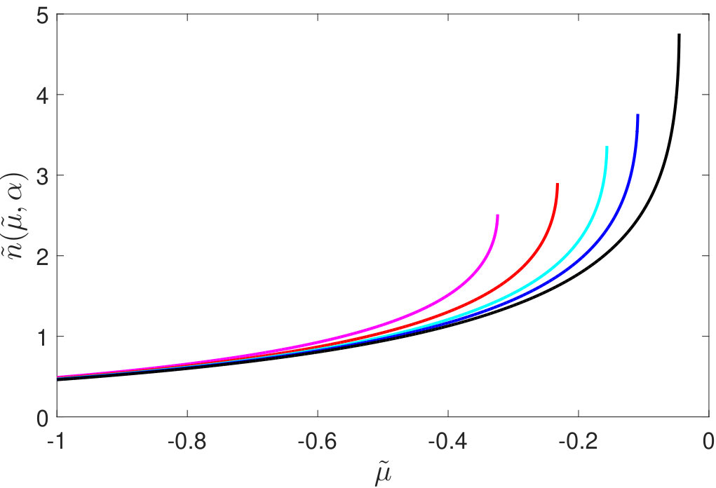 Figure 1
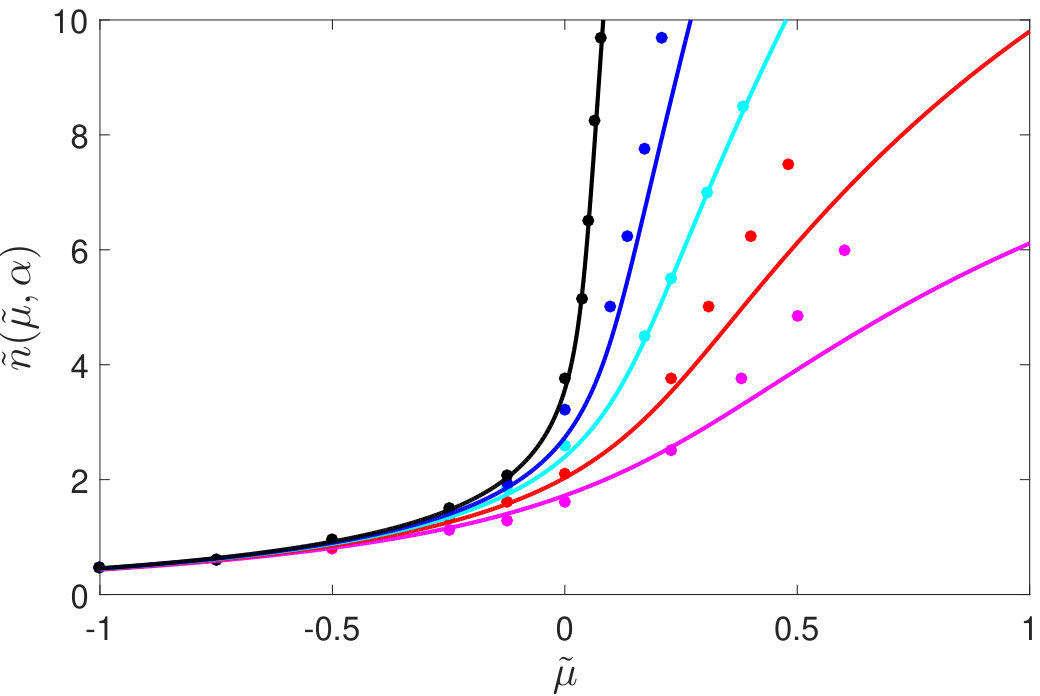 Figure 2
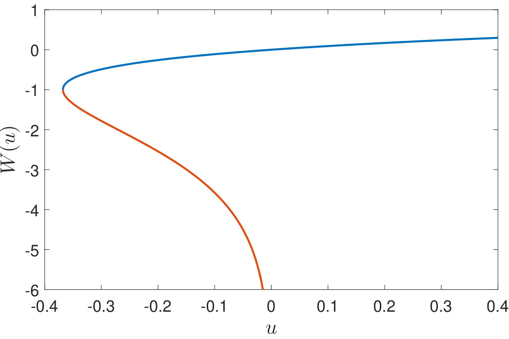 Figure 3
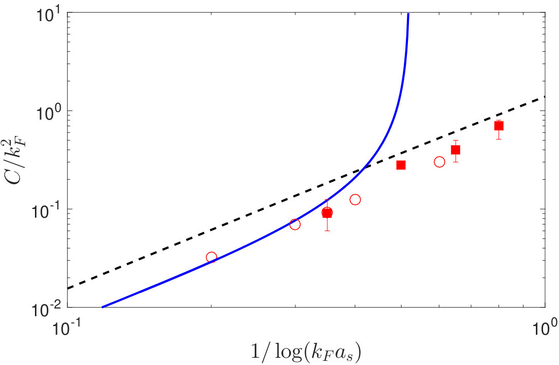 Figure 4
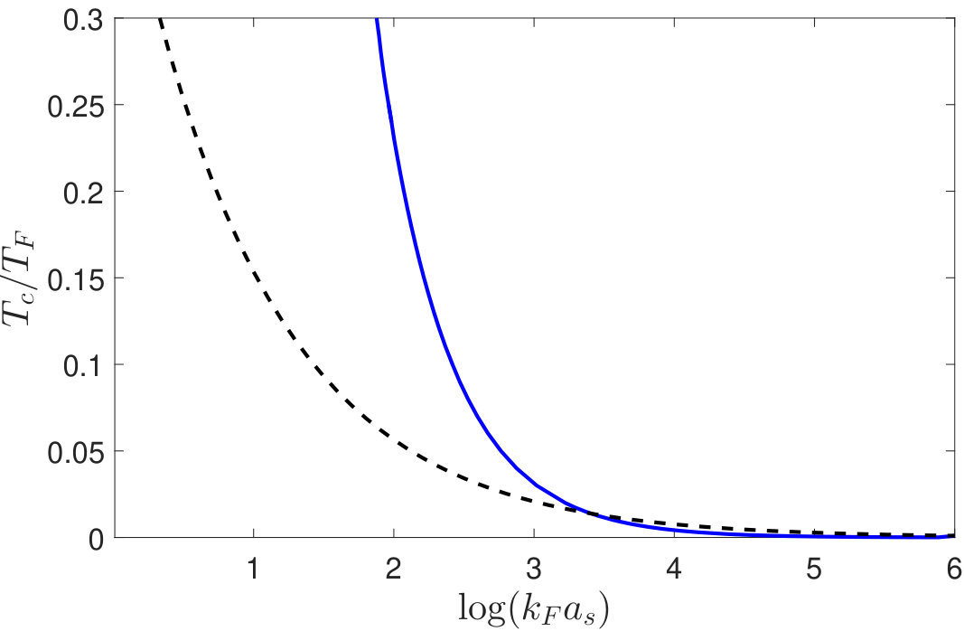 Figure 5
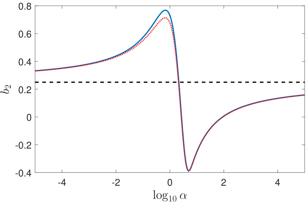 Figure 6
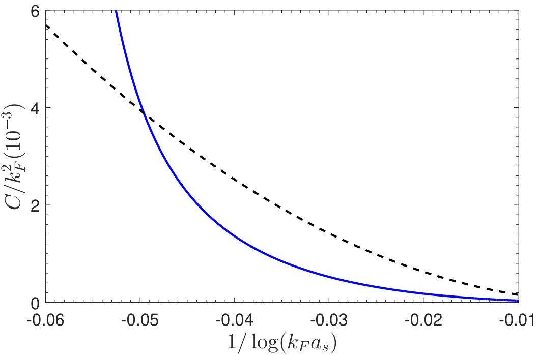 Figure 7
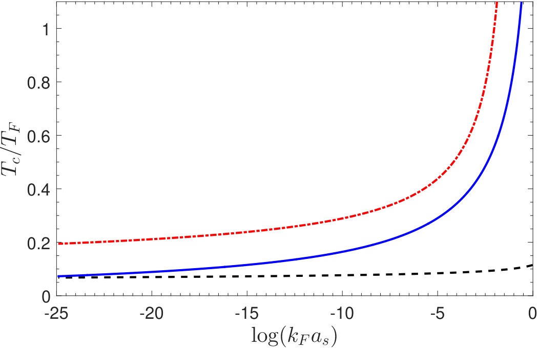 Figure 8
| weak coupling | strong coupling | |||||||
| repulsive | 0 | |||||||
| attractive | ||||||||
Peer Reviews
No public reviews on file for this paper yet. If you reviewed it on a platform where reviews are public (OpenReview, ICLR, NeurIPS, ICML), you can paste yours below so the community can read it here.
Videos
No videos yet. Explain this paper in a talk, walkthrough, or lecture? Add one.
Two-dimensional Bose and Fermi gases beyond weak coupling
Guilherme França
Department of Physics, Cornell University, Ithaca, NY
André LeClair
Department of Physics, Cornell University, Ithaca, NY
Joshua Squires
Department of Physics, Cornell University, Ithaca, NY
Abstract
Using a formalism based on the two-body S-matrix we study two-dimensional Bose and Fermi gases with both attractive and repulsive interactions. Approximate analytic expressions, valid at weak coupling and beyond, are developed and applied to the Berezinskii-Kosterlitz-Thouless (BKT) transition. We successfully recover the correct logarithmic functional form of the critical chemical potential and density for the Bose gas. For fermions, the BKT critical temperature is calculated in BCS and BEC regimes through consideration of Tan’s contact.
pacs:
05.45.Mt, 03.75.Mn, 03.67.-a
I I. Introduction
The absence of conventional long range order in two-dimensional (2D) systems is well known to be a consequence of low energy fluctuations MerminWagner ; Hohenberg . Phase transitions at finite temperature in 2D are instead marked by a topolgical order as described by Berezinskii, Kosterlitz, and Thouless (BKT) Berezinskii ; KT . Quasi long range order is exhibited below the BKT transition temperature, where spatial correlations of the order parameter decay algebraically rather than exponentially. The destruction of this ordering, due to the unpairing of vortices, has been observed experimentally using atomic gases Hadzibabic .
Ultracold atomic gases are well suited for the exploration of BKT theory, as they can be effectively constrained to 2D Martiyanov ; Frohlich ; Makhalov ; Sommer ; Tung ; HaHung ; Rammelmuller ; Boettcher using an optical lattice or harmonic trap, and because their interactions are highly tunable through the use of Feshbach resonances. Theoretical studies of BKT physics in two dimensions using quantum gases are numerous. Fermi gases have been used to explore Cooper pairing and superconductivity in 2D Randeria1 ; Randeria2 , as well as the normal Fermi liquid phase Engelbrecht ; Engelbrecht2 ; Drut . The superfluid transition and critical point of the 2D Fermi gas have also been treated Petrov2 ; Botelho ; Miyake . Bose Einstein condensation in 2D, particularly at weak coupling, has been widely studied Fisher ; Holzmann . The critical point of the 2D Bose gas has been obtained in this limit through classical theory Popov ; Prokofev1 ; Prokofev2 , and with a renormalization group (RG) approach Rancon . An RG analysis has also been used to examine the ground state of the Bose gas in arbitrary dimension Kolomeisky .
In this paper we apply the formalism developed in PyeTon to study two-dimensional Bose and Fermi gases with both attractive and repulsive interactions. Inspired by the Yang-Yang equations of the Thermodynamical Bethe Ansatz YangYang , the formalism is centered around an integral equation with a kernal based on the logarithm of the two-body S-matrix. The main advantage of our approach is that the two-dimensional integral equation admits approximate analytic solutions in terms of the Lambert function. Furthermore these approximate solutions remain useful beyond weak coupling, and as detailed in section III, they can be used to calculate any thermodynamic quantity of interest. In this work we primarily use this correspondence to calculate the critical points of the BKT transition for both Bose and Fermi gases. Below we summarize our chosen models, couplings, and formalism before describing our main results in sections IV and V.
II II. Renormalization Group, physical couplings, and thermodynamic scaling functions
The models considered in this paper are the simplest models of non-relativistic bosons and fermions with quartic interactions. The bosonic model is defined by the following action for a complex scalar field :
[TABLE]
For fermions, due to the fermionic statistics, one needs at least a 2-component field :
[TABLE]
In both cases, positive (negative) corresponds to repulsive (attractive) interactions.
Although classically the coupling is dimensionless, in the quantum theory it is not exactly marginal, i.e. it has a renormalization group (RG) flow. One way to determine the beta function is to calculate the exact 2-body S-matrix PyeTon . Multi-loop Feynman diagrams are divergent, and can be regularized with an ultraviolet cutoff in momentum space . The result is
[TABLE]
The above beta function is exact, i.e. there are no higher order corrections. It is characteristic of Berezinskii-Kosterlitz-Thouless transitions. For positive, it is marginally irrelevant in that at low energies flows to zero, whereas negative is marginally relevant, i.e. flows to .
There is a characteristic momentum scale in the problem, which plays the role of the physical coupling,
[TABLE]
Since it is an RG invariant
[TABLE]
The two-body S-matrix can be expressed entirely in terms of this scale:
[TABLE]
where is the relative momentum of the two incoming particles. Note that because the two-body S-matrix can be calculated to all orders in the coupling, the second virial coefficient can be obtained exactly within our formalism, as explained in the appendix.
We will define the physical scattering length as
[TABLE]
In two dimensions, this choice is really just a convention. Comparing the scattering amplitude based on the above S-matrix and the calculation in Rancon , the convention in the latter is , where is the Euler-Mascheroni constant.
Thus as , i.e. approaches zero from above, the scattering length . On the other hand as . Strong coupling, just corresponds to a finite . Note that a negative scattering length is not physically possible, unlike in three dimensions. For reference, the parameters in the weak and strong coupling limits are summarized in Table 1.
It is not physically meaningful to express properties in terms of since it is not a renormalization group invariant; rather they should be expressed in terms of the scattering length . At finite temperature and density, it is convenient to define the dimensionless variables:
[TABLE]
where is the thermal de Broglie wavelength and the chemical potential. The scaled density
[TABLE]
is a function of and . For the full equation of state involving pressure, one also needs the free energy density:
[TABLE]
where is defined below. With the above normalization, for a free boson at zero chemical potential. In two dimensions the Fermi wave-vector is and the Fermi temperature , which implies . In units of the Fermi energy, the energy per particle takes the form
[TABLE]
For comparison with other calculations and experiments, it is also useful to define a physical coupling as
[TABLE]
The above definition is such that at weak coupling .
III III. Formalism
In the formalism developed in PyeTon , thermodynamic functions are determined by a pseudo-energy which represents a single particle energy in the presence of interactions with all the other particles in the gas. The occupation numbers take the free particle form
[TABLE]
where () corresponds to bosons (fermions). Consistent re-summation of all two particle interactions leads to an integral equation for . It is convenient to define the function
[TABLE]
where . Without interactions, . With interactions satisfies the non-linear integral equation
[TABLE]
where , and refers to bosons or fermions, respectively, with . Henceforth without a subscript will refer to . The fermionic case will be studied in section V.
The kernel is related to the logarithm of the two-body S-matrix,
[TABLE]
Rescaling , the scaling functions are then given by the following integrals ():
[TABLE]
The integral equation (16) then becomes
[TABLE]
where the kernel is
[TABLE]
The free theory limit corresponds to both, () and (). It will be convenient to write the integral equation (20) as
[TABLE]
where
[TABLE]
In theory the integral equation (16) is valid for all interaction strengths and temperatures, including . However, as our formalism only includes a pseudo-energy for single particles, the integral equation is only solvable in the absence of bound states, limiting its applicability at zero temperature. Low temperature results are accurate only if the gas remains in the normal phase. As a concrete example, we calculated Tan’s contact for the attractive Fermi gas in the normal phase for temperatures as low as (see Figure 5 and the discussion in Section V).
We also expect solutions of the integral equation to become less reliable if the coupling is large enough to result in appreciable many-body interactions, as only two-body effects are considered. If we take as a measure of strong verses weak coupling the constant defined in (13), then because of the logarithm, requires (for repulsive interactions) a very large , on the order of (see below). For such large , in practice we can disregard the momentum dependence of the above kernel. We checked numerically that retaining the dependence did not substantially alter our results below. Thus, henceforth
[TABLE]
is a constant that differs in sign depending on whether the interaction is attractive or repulsive.
IV IV. Bosons
Since the kernel is a constant, is also a constant. The integral over can be performed and the integral equation (22) becomes the transcendental equation
[TABLE]
The equation of state is then
[TABLE]
Given the solution to (25) for as a function of , the above equation determines how the density depends on the chemical potential and temperature.
For very weak coupling, , and (25) can be approximated as
[TABLE]
which can be expressed in terms of the Lambert -function. The function by definition satisfies
[TABLE]
One then has the following solution of the transcendental equation:
[TABLE]
Thus
[TABLE]
For real , has two real valued branches, as shown in Figure 1 below. If there is only the principal branch denoted by , and if we have the principal branch and also the secondary branch . The two branches only coincide when , where .
IV.1 A. Repulsive Bosons
For the repulsive case the argument of is positive and one should chose the principle branch, henceforth simply denoted as .
In order to compare with other theories and experiments, we wish to plot as a function of for various . The above equations give explicit expressions in terms of rather than . However the primary variation of comes from the variation of . Therefore we plot as a function for a fixed . Along such a curve is nearly constant, thus it is meaningful to associate each fixed- curve with . Our results, which use the approximation (30), are compared to experimental data in Figure 2 for ranging between and . Due to the logarithms, this requires a very large range of . For instance corresponds to whereas coincides with .
As the behavior is of a free gas . There are significant downshifts at finite which increase with . These results compare reasonably well with the measurements in HaHung .
At some critical density the gas is known to become a superfluid. In order to motivate our analysis of the critical point, let us consider ordinary BEC of free particles in three spatial dimensions. Here the kernel , and , which implies . At the critical point the occupation number diverges, implying . This property is reflected in the analytic properties of the density as a function of as follows. One has where is the polylogarithm. The latter has a branch cut along the real axis where the density develops an imaginary part. Therefore the critical point is and where is the Riemann zeta function. In two dimensions this leads to which diverges due to the pole of at .
For a two dimensional interacting gas, as in the 3D non-interacting case, at the critical point the scaled density develops an imaginary part. This occurs for where the RHS of (25) has a branch cut. In order to study this analytically using known functions, we consider the approximate solution of (25) given by (30). Taking implies
[TABLE]
Since the argument of is arbitrarily large and positive for weakly coupled repulsive interactions, the approximation can be used, giving
[TABLE]
The solution to the above equation can again be expressed in terms of the Lambert function
[TABLE]
Noting to second order, for large , , one can use the above equation and (26) to compute the critical chemical potential and density:
[TABLE]
We now compare (34) with known results and experiments. From the scattering length definition given by (8) we see . This leads to
[TABLE]
with . The above functional dependence on agrees with Prokofev1 ; HaHung except for the constants inside the logarithm, where it was found that and We do not understand the reason for this discrepancy. The simplest explanation is that we are neglecting intrinsic 3-body interactions and higher; however it is hard to see how these would lead to the same functional form as in (35) with just modifications of the ’s. It seems more likely to be an effect of our simplifications of the kernel in the integral equation, which effectively neglected its momentum dependence in the limit of large . Although we did not find any significant evidence of this numerically, it remains possible that we did not treat the integral equation properly in the infra-red, i.e. low .
IV.2 B. Attractive Bosons
For attractive interactions in the weak coupling limit, (24) is positive, and . In this regime there exists only very small regions of parameter space where there is a solution to (25). This instability is reflected in the equation of state, as shown in Figure 3.
At the critical point, again becomes complex. The main difference in repeating the analysis of the previous section is now, for attractive interactions, the argument of in (30) is arbitrarily small and negative and one must choose the secondary branch rather than the principle branch. After setting we find
[TABLE]
Utilizing the asymptotic expansion of the secondary branch gives
[TABLE]
from which it follows
[TABLE]
As in the repulsive case the critical density can be computed by inserting the above expression into (26). Using the asymptotic expansion of a second time results in
[TABLE]
V V. Fermions
In the fermionic case the kernal . The analogs of (25) and (26) for fermions at weak coupling are then
[TABLE]
and
[TABLE]
Mirroring our treatment of bosons, we find approximate solutions for in the attractive ()
[TABLE]
and repulsive ()
[TABLE]
regimes in terms of the Lambert function.
A. Attractive Fermions
A useful quantity to calculate is the contact parameter, , which is set by the antiparallel spin pair correlation function at short distances (). Tan’s relations provide a connection between , and thus the short range interactions of the system, and macroscopic quantities such as the pressure of the gas Tan . One can define a dimensionless contact in terms of a derivative of the energy with respect to the interaction parameter
[TABLE]
Note since this derivative can be calculated explicitly with our formalism. Using the approximations given by (41) and (42):
[TABLE]
where .
For the 2D attractive fermi gas, the contact was recently measured experimentally at Frohlich . In Figure 4 below we compare as calculated with our approximations to experiment, as well as to a Fermi liquid theory result Engelbrecht2 . Our compares favorably with the experimental measurements until diverging abruptly as .
Since is proportional to the number of atomic pairs, which follows from the relation between the contact and Werner , a divergence in may signal a phase transition. Identifying the critical point of the BKT transition with a diverging yields the phase diagram shown in Figure 5.
In the 2D BCS limit , the critical temperature of the superfluid transition has been calculated using mean field theory Petrov2 ; Miyake
[TABLE]
Fitting our phase boundary to a second order model
[TABLE]
gives and . Our results begin to significantly depart from those of mean field theory around which corresponds to . This is well into the regime of strong interactions, so it’s unsurprising we deviate from a mean field theory prediction.
Before considering repulsive interactions, we note that Monte Carlo simulations have been used to calculate both the contact and energy per particle at on both sides of the BEC-BCS crossover. For example, in Bertaina for , the normalized energy per particle is reported as . To compare to this data we calculate using (12) at low temperature. For convenience we take , which fixes the density . Since the interaction parameter only depends on and , setting uniquely determines . With and known, a corresponding can be found numerically, and used to calculate the energy per particle. Utilizing the approximations (41) and (42) throughout, we obtain . Although is provided for a range of interaction strengths, most of the data presented in Bertaina occurs in the presence of a bound state, which our formalism is not suited to handle.
B. Repulsive Fermions
While we don’t have experimental data to compare to on the BEC side, the contact is equivalent to (45) with in place of . As in the attractive case, a sharp increase in is observed (see Figure 6) which we take as indication of a phase transition. In the BEC limit of , the predicted critical temperature is
[TABLE]
with Prokofev1 ; Petrov2 . We instead find to be more consistent with the value from (35), as shown in Figure 7. The return of this discrepancy is expected based on the analysis in section IV, as in this limit the system behaves as a weak Bose gas.
VI VI. Conclusions
The S-matrix-based formalism developed in PyeTon has been applied to two-dimensional Bose and Fermi gases. The main obstacle in utilizing this method to extract measurable thermodynamic functions is solving an integral equation whose kernal takes a particularly complicated form in two dimensions. This makes exact solution of the integral equation an impossible task, and numerical treatments computationally intensive. Fortunately, in the limits and the momentum dependence of the kernal becomes irrelevant, and elegant solutions of the integral equation can be written in terms of the Lambert W function.
While we initially anticipated these approximate solutions would only remain valid in the limit of extremely weak coupling, it turns out is a more appropriate measure of coupling strength than , due to its explicit density dependence. For strong coupling, which is reached in the or limit depending on the sign of the interaction.
For bosons, we were able to recover the well-established logarithmic functional form of the critical density and chemical potential with the Lambert approximation, up to a constant obtained with Monte Carlo methods Prokofev1 . For fermions our approximations result in an explicit expression for the contact parameter, from which the critical temperature of the BKT transition has been deduced. This novel approach agrees with known weak coupling mean field theory calculations Miyake ; Petrov2 .
As two-dimensional gases are poised to garner even greater attention in the near future, we hope our explicit analytic results are found to be useful.
VII Acknowledgments
We thank John Stout for collaboration in the early stages of this work which led to the Appendix.
VIII Appendix: Virial expansion
We did not use the following results in the body of the article, however we present them here since they may be useful in future studies.
The virial expansion is formally defined as a series expansion of in powers of the fugacity :
[TABLE]
where the second relation follows from . In the free theory, the series expansion of the poly-logarithm gives .
As explained in Roditi our formalism gives the corrections to and :
[TABLE]
[TABLE]
The second virial coefficient is exact, whereas is not since it does not contain the intrinsic 3-body physics. Hence we only consider . Rescaling , and making the change of variables , , the integral factorizes and the integral over is simply a gaussian. The result is
[TABLE]
where and for bosons and for fermions. To a good approximation,
[TABLE]
Plots of are shown in Figure 8. Note that it changes sign at . As expected, the free theory value is approached in both limits and .
The reference list from the paper itself. Each links out to its DOI / PubMed record.
- 1(1) N. D. Mermin and H. Wagner, Absence of ferromagnetism or antiferromagnetism in one- or two-dimensional isotropic heisenberg models , Phys. Rev. Lett. 17 , 1133-1136 (1966).
- 2(2) P. C. Hohenberg, Existence of long-range order in one and two dimensions , Phys. Rev. 158 , 383-386 (1967)
- 3(3) V. Berezinskii, Sov. Phys. JETP 34 610 (1972).
- 4(4) J. Kosterlitz and D. Thouless, J. Phys. C 6 1181 (1973).
- 5(5) Z. Hadzibabic, P. Krüger, M. Cheneau, B. Battelier, and J. Dalibard, Berezinskii-Kosterlitz-Thouless crossover in a trapped atomic gas Nature (London) 441 , 1118 (2006).
- 6(6) K. Martiyanov, V. Makhalov, and A. Turlapov, Observation of a two dimensional Fermi gas of atoms , Phys. Rev. Lett. 105 , 030404 (2010).
- 7(7) A. T. Sommer, L. W Cheuk, M. J. H. Ku, W. S. Bakr, and M. W. Zwierlein, Evolution of fermion pairing from three to two dimensions , Phys. Rev. Lett. 108 , 045302 (2012).
- 8(8) B. Fröhlich, M. Feld, E. Vogt, M. Koschorreck, M. Kohl, C. Berthod, and T. Giamarchi, Two-dimensional Fermi liquid with attractive interactions , Phys. Rev. Lett. 109 , 130403 (2012).