Triangle mechanisms in the build up and decay of the $N^*(1875)$
Daris Samart, Wei-hong Liang, Eulogio Oset

TL;DR
This paper investigates the $N^*(1875)$ resonance using a multichannel unitary approach, revealing significant decay channels and the importance of triangle diagrams, with implications for experimental analysis.
Contribution
It introduces a multichannel unitary scheme incorporating triangle diagrams to study the $N^*(1875)$ resonance, highlighting the role of specific decay channels and singularities.
Findings
Large decay width to $ ext{Σ}^* K$ channel
Triangle singularity at the resonance energy
Significant role of $N \sigma$ in $ ext{π} ext{π}$ mass distributions
Abstract
We have studied the resonance with a multichannel unitary scheme, considering the and , with their interaction extracted from chiral Lagrangians, and then have added two more channels, the and , which proceed via triangle diagrams involving the and respectively in the intermediate states. The triangle diagram in the case develops a singularity at the same energy as the resonance mass. We determine the couplings of the resonance to the different channels and the partial decay widths. We find a very large decay width to , and also see that, due to interference with other terms, the channel has an important role in the mass distributions at low invariant masses, leading to an apparently large decay width. A discussion is done,…
Click any figure to enlarge with its caption.
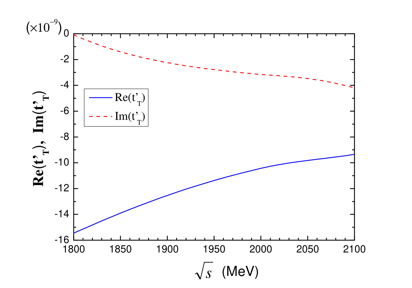 Figure 1
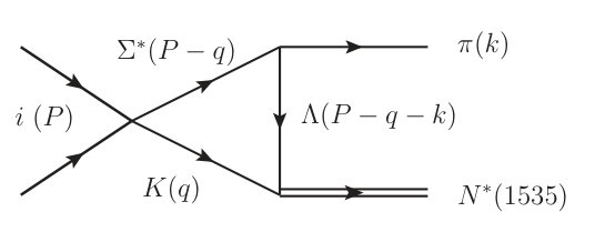 Figure 1
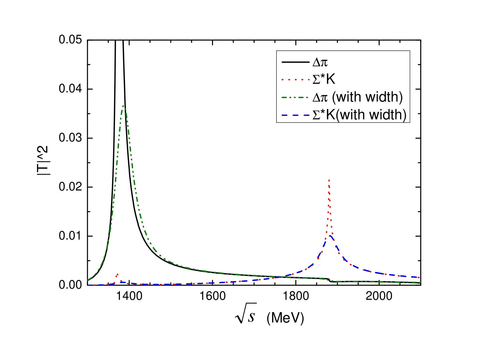 Figure 12
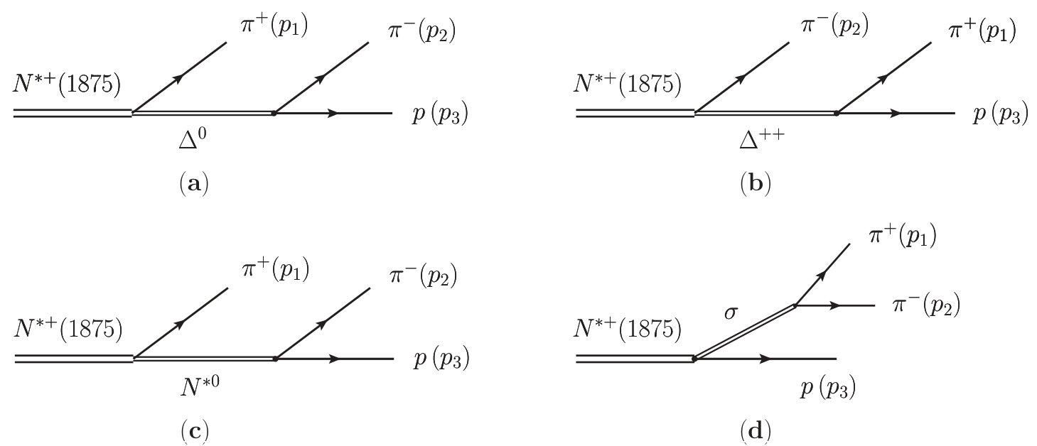 Figure 17
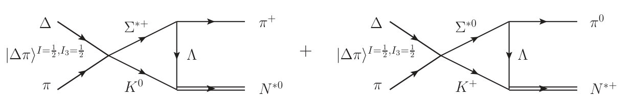 Figure 2
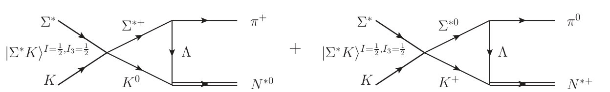 Figure 3
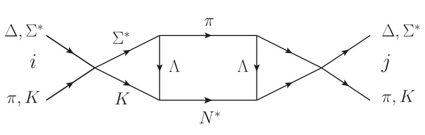 Figure 4
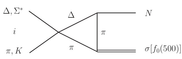 Figure 5
 Figure 6
 Figure 7
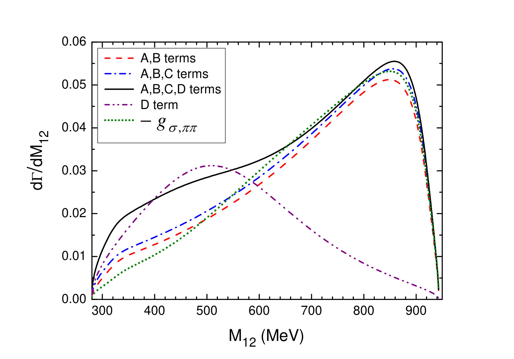 Figure 11
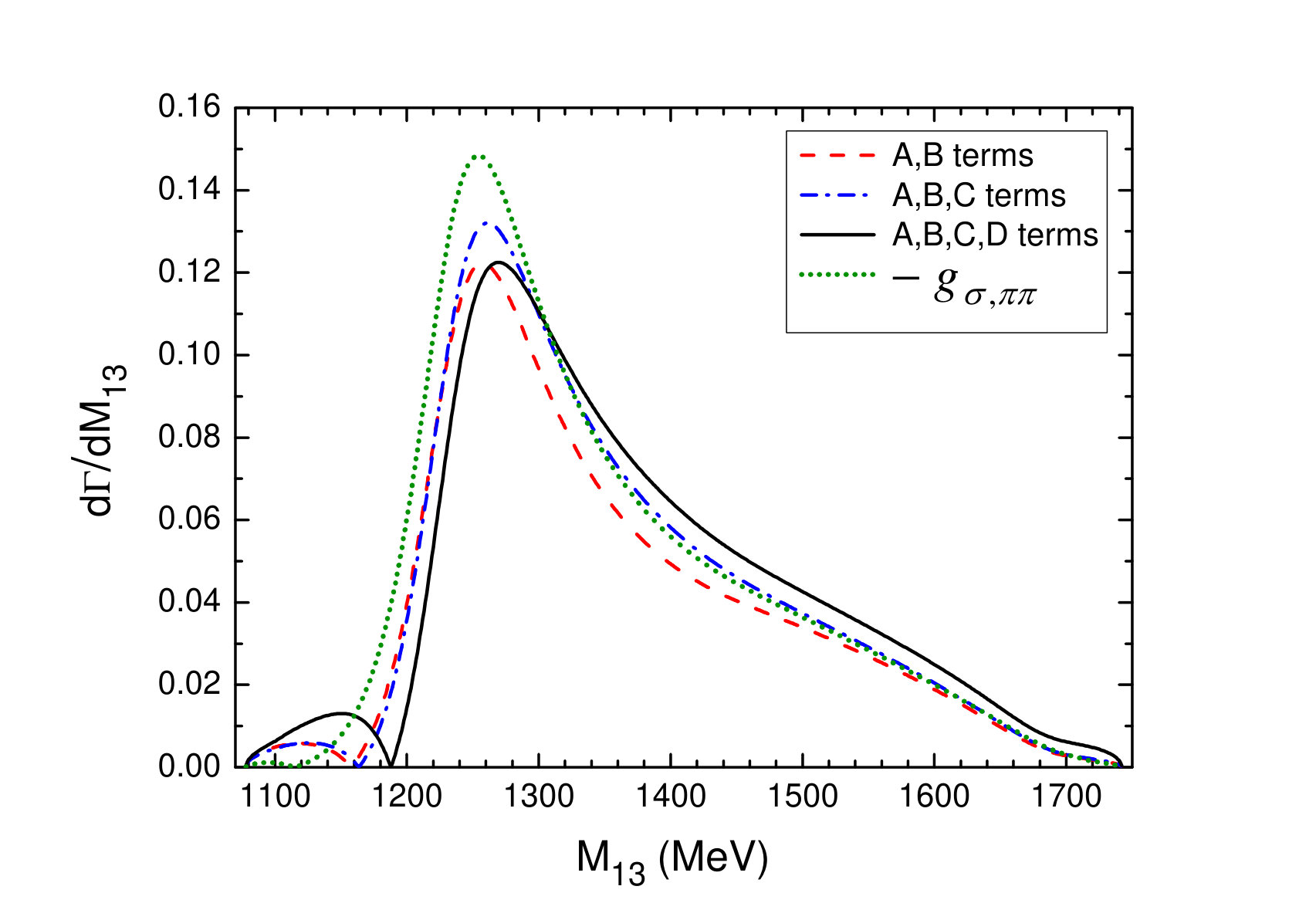 Figure 12
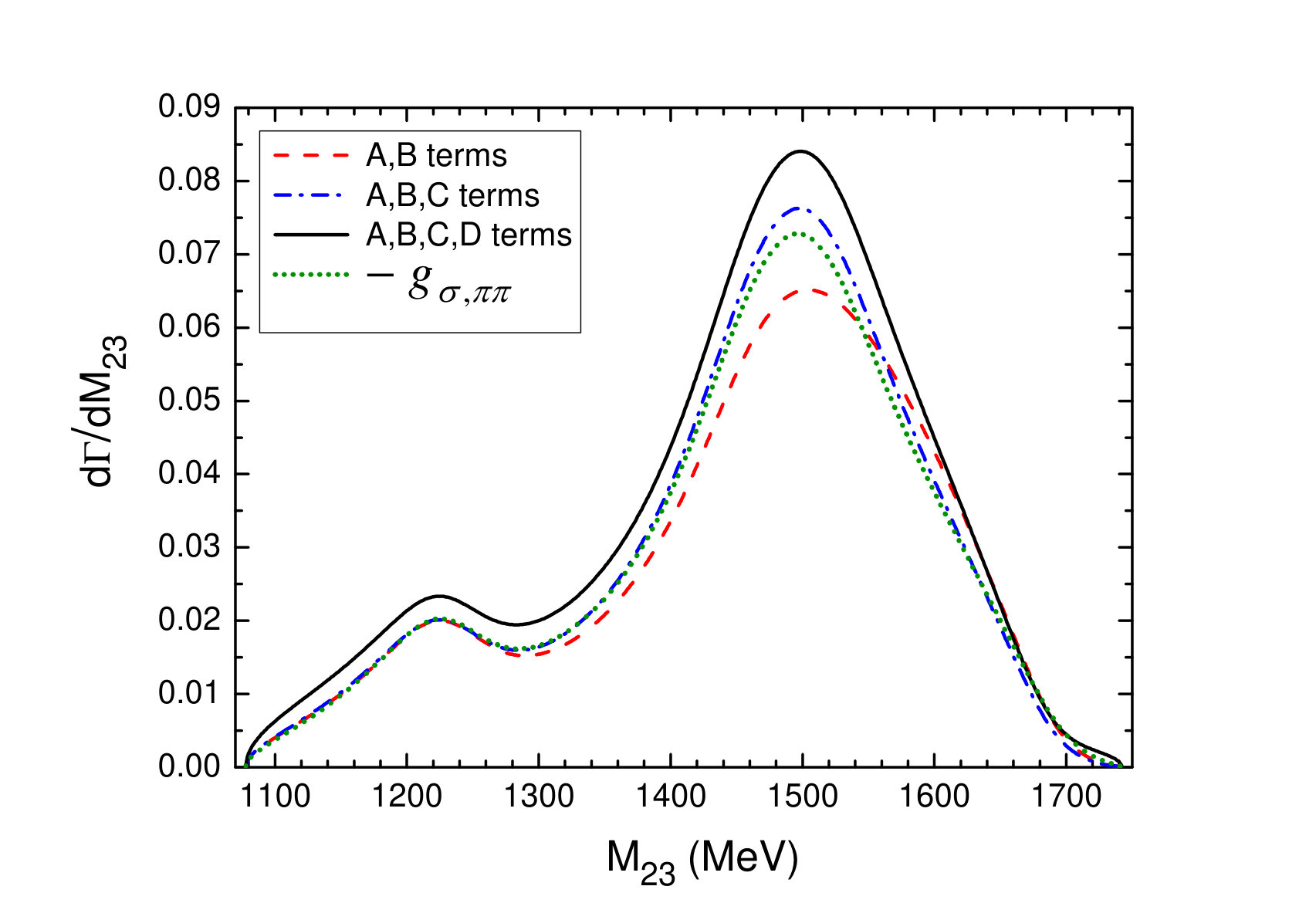 Figure 13
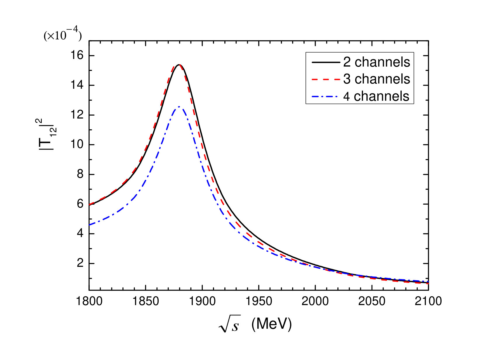 Figure 14
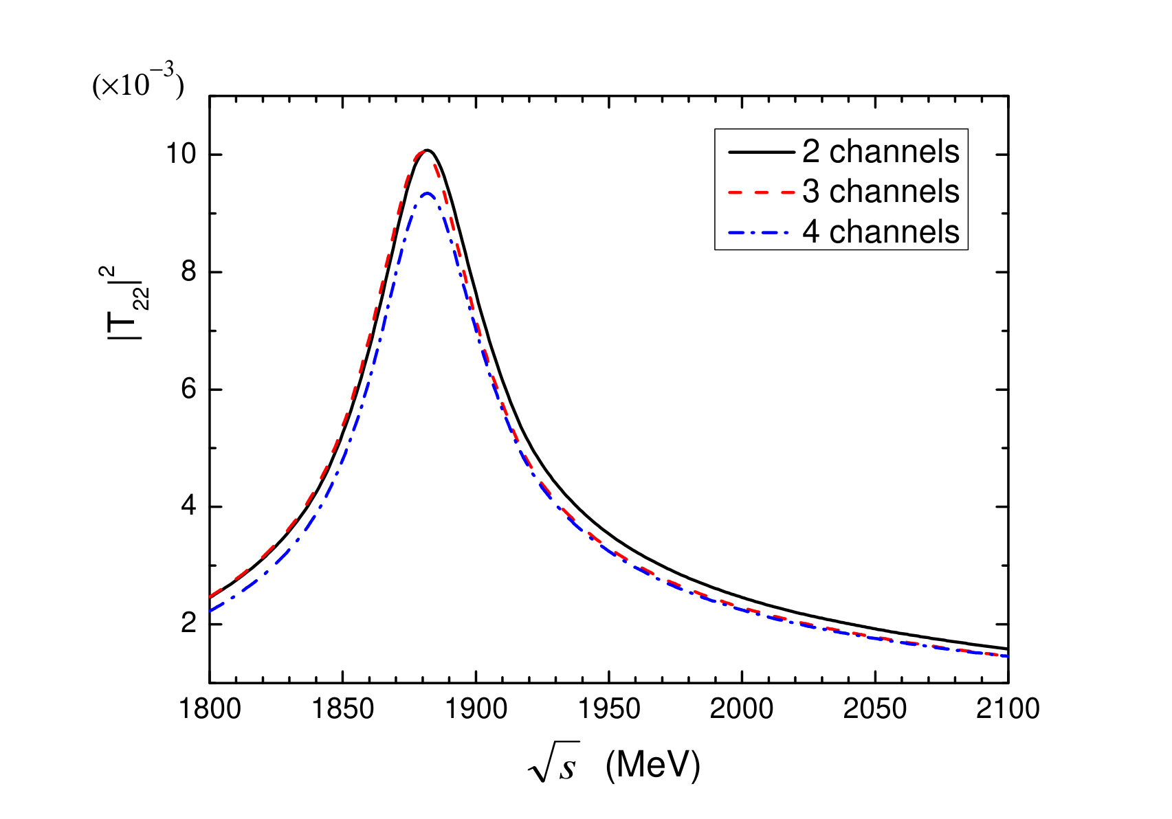 Figure 15
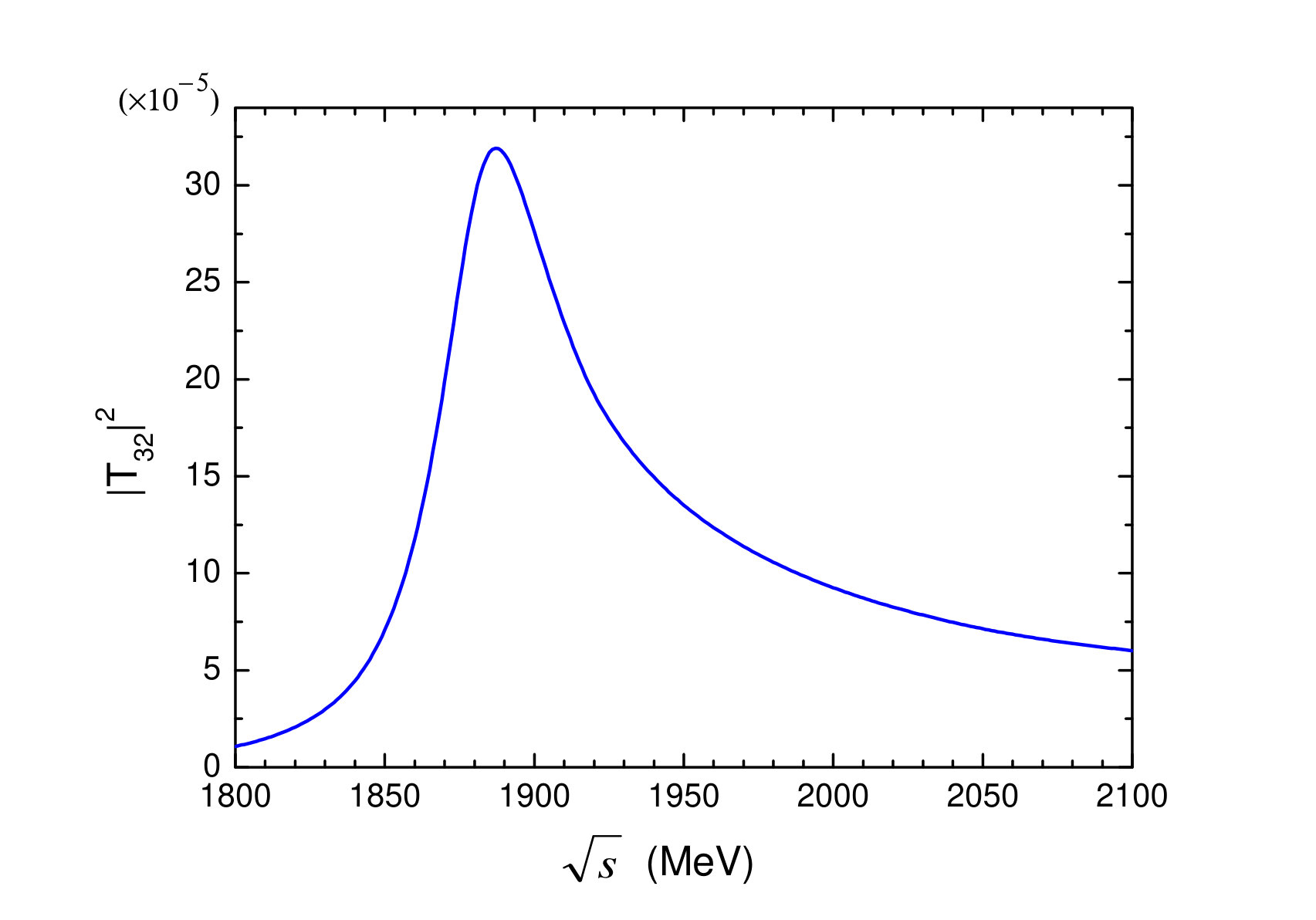 Figure 16
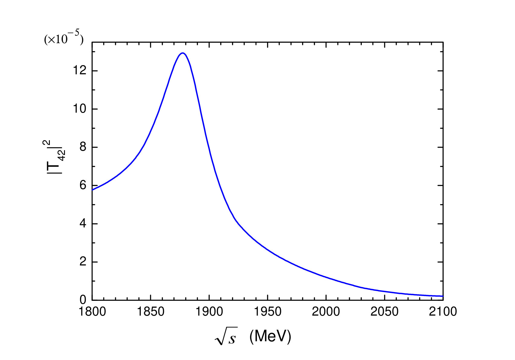 Figure 17
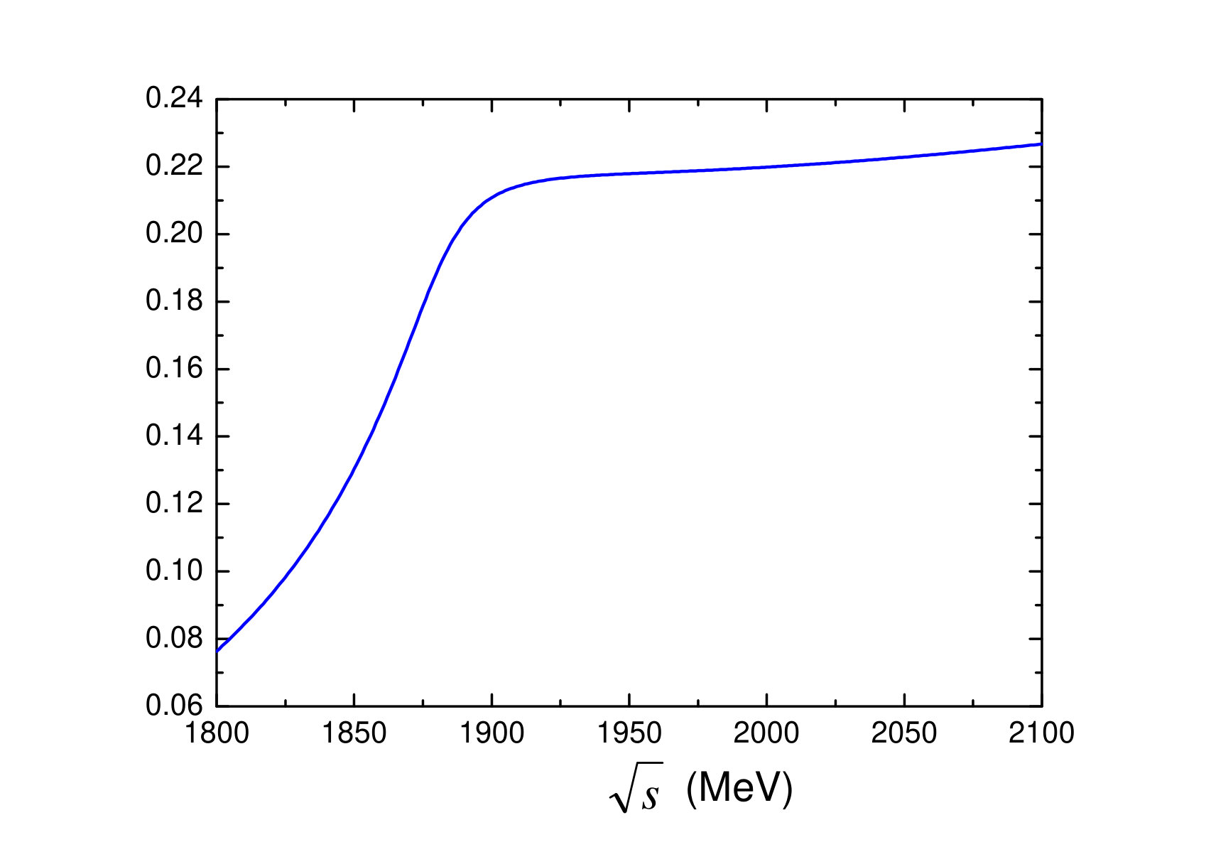 Figure 18
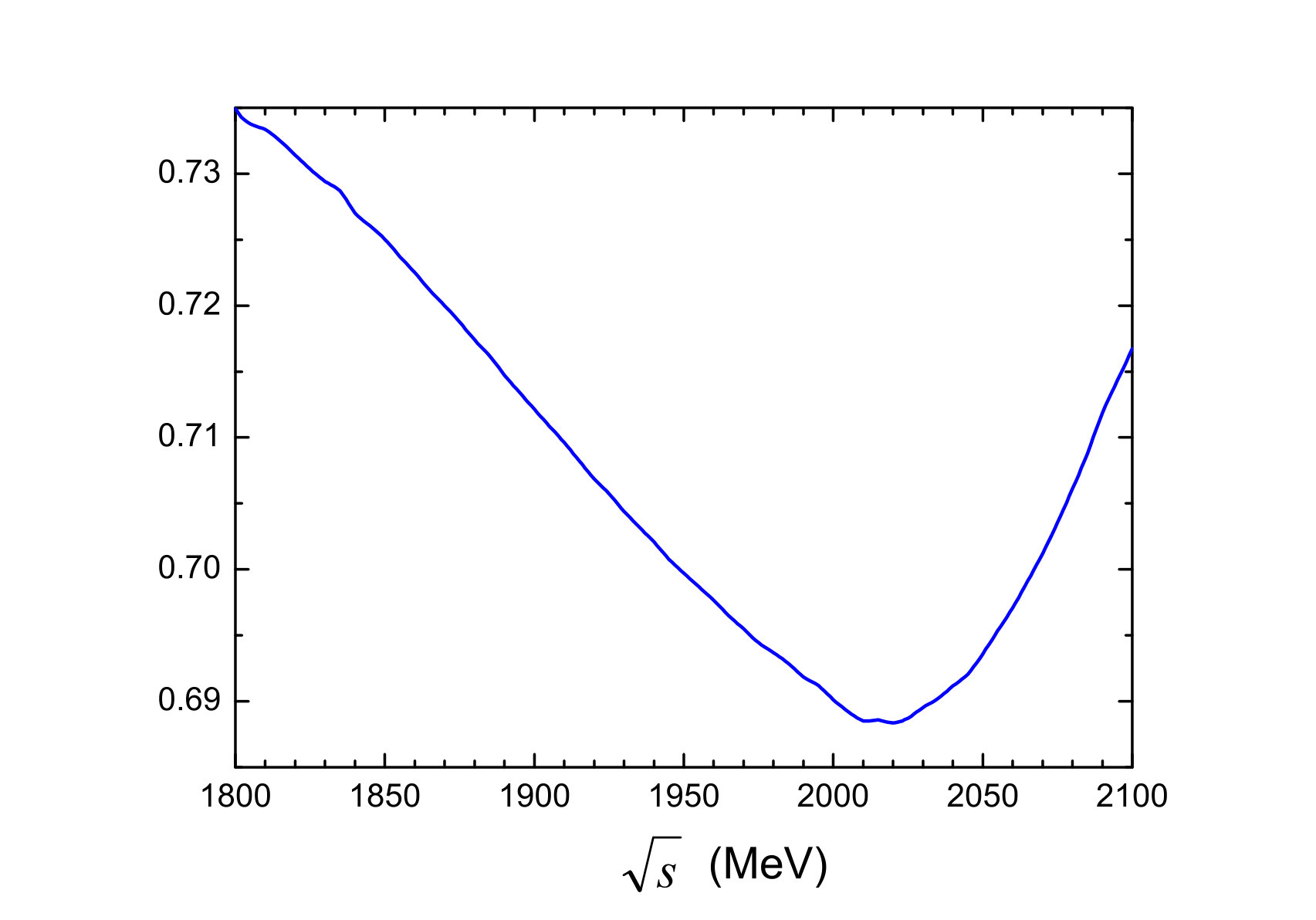 Figure 19
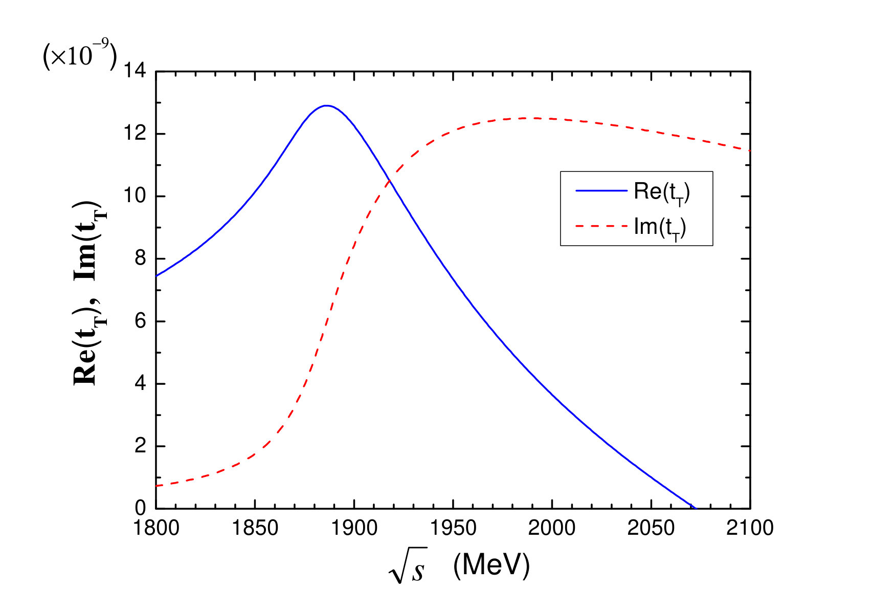 Figure 20
| 5 | 2 | |
| 2 | 2 |
Peer Reviews
No public reviews on file for this paper yet. If you reviewed it on a platform where reviews are public (OpenReview, ICLR, NeurIPS, ICML), you can paste yours below so the community can read it here.
Videos
No videos yet. Explain this paper in a talk, walkthrough, or lecture? Add one.
Triangle mechanisms in the build up and decay of the
Daris Samart
Department of Applied Physics, Faculty of Sciences and Liberal arts, Rajamangala University of Technology Isan, Nakhon Ratchasima, 30000, Thailand
Center Of Excellent in High Energy Physics & Astrophysics, Suranaree University of Technology, Nakhon Ratchasima, 30000, Thailand
Departamento de Física Teórica and IFIC, Centro Mixto Universidad de Valencia-CSIC Institutos de Investigación de Paterna, Aptdo. 22085, 46071 Valencia, Spain
Wei-Hong Liang
Department of Physics, Guangxi Normal University, Guilin 541004, China
Eulogio Oset
Departamento de Física Teórica and IFIC, Centro Mixto Universidad de Valencia-CSIC Institutos de Investigación de Paterna, Aptdo. 22085, 46071 Valencia, Spain
Abstract
We have studied the resonance with a multichannel unitary scheme, considering the and , with their interaction extracted from chiral Lagrangians, and then have added two more channels, the and , which proceed via triangle diagrams involving the and respectively in the intermediate states. The triangle diagram in the case develops a singularity at the same energy as the resonance mass. We determine the couplings of the resonance to the different channels and the partial decay widths. We find a very large decay width to , and also see that, due to interference with other terms, the channel has an important role in the mass distributions at low invariant masses, leading to an apparently large decay width. A discussion is done, justifying the convenience of an experimental reanalysis of this resonance to the light of the findings of the paper, using multichannel unitary schemes.
I Introduction
The (1875) () is relatively new in the PDG pdg . Quoting from the latest PDG edition, “Before the 2012 Review, all evidence for a state with a mass above 1800 MeV was filed under a two star (2080). There is now evidence from Ref. anisovich for two states in this region, so we have split the older data (according to mass) between a three-star (1875) and a two-star (2120).” The mass of the PDG is 1820-1920 MeV (1875 MeV PDG estimate) and the width 250 70 MeV. Quoting directly from Ref. anisovich , the mass is 1880 20 MeV and the the width 200 70 MeV. A more recent experiment sokhoyan agrees with these values with 1875 20 MeV for the mass and 200 25 MeV for the width. The most important decay modes are (15-25%), (10-35%), mostly in -wave, and () (30-60%).
It is interesting to recall that prior to its acceptance as a new resonance, a peak in the amplitudes was observed around 1875 MeV from the study of the pseudoscalar meson-baryon decuplet interaction in Ref. sarkar . For the case of strangeness and isospin , the coupled channels and were used, and the interaction was obtained from the meson-baryon Lagrangians of Ref. manohar . The peak appears at the threshold and it was identified as a threshold effect, not a genuine resonance. One should note that the identification of threshold effects with resonances is quite common and one has a good example with the (980) which is catalogued as a resonance, but it shows both theoretically npa and experimentally kornicer as a cusp effect with no clear pole associated to it.
In the present paper we retake the work of Ref. sarkar and include triangle mechanisms associated to the main building channels , , which lead to new channels and . The first channel has not been measured yet, but the second channel is, together with the main decay channel of the resonance. An effective transition potential is constructed from the , channels to the and , and a four channel problem is then solved with a unitary coupled channel scheme, leading to a resonant peak around 1875 MeV in the amplitudes from where we extract the coupling of the resonance to the different channels and the partial decay widths to these channels.
Triangle diagrams have for long been part of hadron physics, but of particular interest are those that lead to singularities in the amplitudes, known as triangle singularities. The concept and detailed study was introduced by Landau landau , but it is precisely now, after much information on the hadron spectrum and reactions has been accumulated, that many examples of triangle singularities show up qzhao . A triangle diagram stems from a particle A decaying into , particle 2 decaying to and particles merging into another particle C. In some cases, when the process can occur at the classical level, a singularity appears in the corresponding Feynman diagram, Coleman-Norton theorem ncol , and the field theoretical amplitude becomes infinity if the intermediate particles are stable. In practice, some of these particles have a finite width and the infinity becomes a peak, with important experimental consequences.
An alternative formulation to the standard method to deal with the triangle singularities is done in Ref. guo , with a different method to perform the integrals and an easy and intuitive rule to determine where the singularities appear.
Recent examples of processes where the triangle singularities are relevant can be seen in the and wu2 ; wu1 ; wu3 . The latter process is isospin forbidden and results largely enhanced due to a triangle singularity involving followed by and fusion of to give the . A more recent example can be seen in the COMPASS collaboration compass , associated to a new resonance “”, which, as hinted in Ref. qzhao and proved in Refs. mikha ; aceti , comes from the decay of the , via a triangle singularity proceeding through , and . Related to this is the recent interpretation of the resonance as a decay mode of the into and vinicius . Another interesting example is the role played by a triangle singularity in the reaction wang . The process , , leads to a peak in the cross section around MeV that solved a standing problem in that reaction.
Similarly, the (1810) is also explained as a consequence of the , and merging into the (1260) geng . Other examples can be found in Refs. hanhart ; achasov ; Lorenz ; adam1 ; adam2 . Renewed interest in the triangular singularities came from the suggestion that the narrow peak of the invariant mass at 4450 MeV seen by the LHCb collaboration penta-ex ; chinese , and interpreted there as a pentaquark state, could be due to a triangle singularity with , , ulfguo ; liu . However, as shown in Ref. guo , for the preferred experimental quantum number of this peak, , , the proceeds with in -wave or -wave and the threshold is exactly 4450 MeV, hence, this amplitude vanishes there on shell and the suggested process cannot be responsible for the observed peak.
In the present work we will show that the process of the , , , develops a triangle singularity precisely at the same mass of resonance and reinforces it. The other interesting finding of this work is that there can also be triangle mechanisms, which, without developing a singularity, can be very important. This is actually the case with , , . We shall see that because of the large strength of all the couplings involved, this process becomes even more important than the and leads to a sizeable partial decay width .
II Formalism
II.1 Brief review of the pseudoscalar meson-baryon decuplet interaction
Following Ref. sarkar , the sector with , is reached with the channels , . In -wave the interaction leads to states. The interaction is given by
[TABLE]
where are energies of the initial and final mesons respectively and the coefficients are given in Table 1.
The scattering matrix is given via the Bethe-Salpeter equation in the matrix form by
[TABLE]
where is the ordinary meson-baryon loop function. The amplitude develops a strong peak around 1500 MeV that was associated in Ref. sarkar to the (1520) resonance. By contrast, this amplitude is very small around 1875 MeV, as a consequence of interference of terms, and it is the amplitude the one that shows as a clear peak around 1875 MeV. In the next subsection we shall include the and channels.
II.2 The (1535) channel
We shall look into the diagram of Fig. 1, where the state stands for and . By looking at equation (18) of Ref. guo , the relationship
[TABLE]
where and are defined by easy analytical expression in Ref. guo , shows the energy at which a triangle singularity appears. One must check Eq. (3) for a mass of the (1535) bigger than . At a mass about 1615 MeV, which is in the range of the (1535) mass considering the width (150 MeV), Eq. (3) shows a solution at 1878 MeV. But a peak in the amplitude develops for smaller masses within the range of the (1535) spectral function, which we shall take into account in the evaluation of the diagram of Fig. 1.
Since we are looking into the states with isospin we must consider in detail, the different charge combinations that enter the evaluation of Fig. 1. This is shown in Figs. 2 and 3, where the state is or , respectively.
We must project all of them into and sum the diagrams. For this, let us recall the sign convention in Ref. sarkar , , of isospin. Hence we have
[TABLE]
We need the coupling and the coupling. The first one is of the type
[TABLE]
where is the spin transition operator from to . The width for is given by
[TABLE]
with
[TABLE]
Hence,
[TABLE]
and using the experimental value for the width we obtain
[TABLE]
The coupling of to we get from Ref. inoue , where the chiral unitary approach has been used to obtain scattering in the region of the (1535). One has
[TABLE]
With these ingredients we can already evaluate the triangle diagrams of Figs. 2 and 3. Considering the isospin coefficients, the sum of the diagrams in Fig. 2, for , , up to the propagators, is given by
[TABLE]
and the full contribution of the loop is given by
[TABLE]
where the last equation defines the triangle integral . The factors , are consequence of using the Mandl and Shaw normalization for the Fermion fields mandl . This integral is performed by doing analytically the integration, and we obtain dias ; guo
[TABLE]
where
[TABLE]
The case of the transition in Fig. 2 proceeds in an identical way, and the only difference with respect to the results of Eq. (12) is that we must substitute by .
We must note that originally the operator appeared for the transition, but upon sum of the intermediate spin components it becomes now in Eq. (12) the spin transition operator from to because the -wave potentials and are independent of the and spins.
Neglecting the width of the in Eq. (13), the integrand in will have poles when
[TABLE]
In principle, in the integral they will give rise to imaginary parts and principal values, via the . However, the cancellations in the principal values will not occur when we are at the extremes of () when . Then a singularity can appear in the integral, triangle singularity (which, occurs for guo ), which however, is rendered finite when the width of the is explicitly considered guo . The integral in the is then convergent, but we perform a cut off in in the rest mass of the , when the chiral unitary approach is done, and we use , suited to the results of Ref. inoue .
We would like to include now the into the coupled channels, together with and . However we can see that while the interaction between and proceeds via -wave, the transition proceeds via -wave with the operator. This is a consequence from the transition of a to which requires change of parity. Yet, it is possible to mix the channels via an effective -wave potential, as done in Refs. garzon ; vectorrev ; uchino1 ; uchino2 . In order to define this effective potential we look at the diagram of Fig. 4, which makes transitions from via an intermediate state.
We can write for the transition amplitude
[TABLE]
In the chiral unitary approach the transition potentials are evaluated for the external lines on shell and we wish to do the same with the new channel . For this purpose, we take the imaginary part of in Eq. (16), which places on shell. Considering that in the transition the pion momentum is in going instead of outgoing as in , we have
[TABLE]
Now we have111Note the order of and the sum over , the spin of the baryon.
[TABLE]
which indicate that we can have transitions in - and -waves. But we are only interested in the -wave and hence we keep the factor in Eq. (17). Thus, effectively we can take
[TABLE]
with
[TABLE]
However, since the triangle singularity is sensitive to the external masses and the has a width of 150 MeV, we make a convolution of Eq. (18) with the spectral function of the , such that
[TABLE]
where , and are obtained substituting in Eqs. (19) and (13). The spectral function of the is given by
[TABLE]
and the factor in Eq. (20) is put for normalization
[TABLE]
The limits of in Eqs. (20) and (22) are taken from to with around one or two. The dependence in Eq. (20) does not effect , hence, we can define
[TABLE]
and a function such that
[TABLE]
then we can construct an effective -wave transition potential
[TABLE]
such that
[TABLE]
This means that using in coupled channels with the extra channel we can effectively incorporate the mechanism of Fig. 4 and when the resonance shows up in the amplitudes we can evaluate the coupling of the resonance to the channel and then the partial decay width into this channel. We will have now a new matrix, containing the of Eq. (1) plus the transition of Eq. (25). We do not include a direct transition assuming such transition would occur via the intermediate states involving the transition which contains the triangle diagram.
In order to take into account the and widths in the functions of Eq. (2) we also do a convolution, as done in Ref. sarkar , with the spectral function of the baryons ,
[TABLE]
II.3 The channel
We can now consider a triangle diagram which involves instead of in the intermediate states. This is depicted in Fig. 5.
The states can now make transition to the , the decays into and then the two pions fuse to give the . The first thing one must check is if this diagram can develop a singularity at some energy . Application of Eq. (3) immediately tells us that this is not the case, and does not vanish for any energy of the original system. However, we have now other elements to make this mechanism particularly relevant. First we can have now transitions that have a weight of a factor 5 (see table 1) instead of 2, as we had before. Second, the coupling is very large and so is the coupling of the to the . The evaluation of the transition proceeds in an analogous way to the previous subsection. First, in analogy to Fig. 2 and Fig. 3 we have now Fig. 6 and Fig. 7.
We need now the state
[TABLE]
and the coupling, similar to Eq. (5)
[TABLE]
with the corresponding isospin Clebsch-Gordan coefficient,
[TABLE]
The coupling , taken to obtain the width, is given by
[TABLE]
corresponding to , very close to standard value used in pion physics, 0.36 ericson . The isospin combination of vertices corresponding to Eq. (11) for Fig. 6 is now given, taking into account Eq. (II.2), by
[TABLE]
For the coupling of the to obtained from the unitary matrix, and unitary normalization ( extra in the wave function of as identical particles) we take
[TABLE]
where we have taken an average between the results of the chiral unitary approach nsd and different results using an analysis of data implementing Roy equations colangelo ; robert (see table 4 of Ref. reviewpel ). With the good normalization to be used in Eq. (35), we have
[TABLE]
Following the argumentation of Eq. (12), we obtain now
[TABLE]
with the nucleon momentum, where is obtained from Eq. (13) by simply changing the masses of the intermediate particles and multiplying the integrand by . The reason for this latter factor is that before in Eq. (12) the factor , factorized outside the integral. Here we have and
[TABLE]
since is an integration variable and is the only vector in the integrand which is not integrated.
For the transition of , we will have the same expression as in Eq. (38) changing to
Finally, in analogy to Eq. (25) we will now have the effective transition potential
[TABLE]
where is defined such that
[TABLE]
with
[TABLE]
with the spectral function
[TABLE]
[TABLE]
[TABLE]
[TABLE]
and , given by the same expressions changing to . For and we take values from Ref. reviewpel
[TABLE]
Now of Eq. (39) provides transitions from () to . As before, we introduce the channel into the coupled channels and have now a matrix for , allowing the , transitions and neglecting direct transition and . For cutoff in the integral of in we take now , suited for the study of interaction npa ; weihong .
II.4 Couplings and partial decay widths
In order to obtain the couplings we look at the amplitudes in Eq. (2), with and plot . We define the mass and width of the resonance the position of the peak and the width of the distribution as a function of close to the peak. In that region we have
[TABLE]
We take the channel as reference and then have
[TABLE]
This defines up to an arbitrary sign, but then the rest of couplings are defined relative to this via
[TABLE]
Once we have the coupling, the partial decay widths are given by
[TABLE]
where is the mass of the final baryon and the one of the resonance and
[TABLE]
with the mass of the final meson in the channels .
The width of all channels is well defined except for the since the resonance is close to threshold and both theoretically and experimentally the determination of in the width is uncertain. With this caveat, we shall check that the sum of all partial decay widths is close to the total width determined from the shape of .
III Results
In Fig. 8, we show the results for as a function of for . We can see that has a peak structure with a peak around . The imaginary part has a different behaviour, and does not show any peak. Actually, would resemble a Breit-Wigner amplitude with a constant magnitude added to the real part, which does not go through zero. The peak observed in is tied to the triangle singularity that one would have in the case that .
In Fig. 9 we show from Eq. (25). This magnitude provides the relative strength of the effective transition potential , with respect to .
We observe that the effective potential rises rapidly up to and stabilizes there. The relative strength with respect to is of the order of 0.22 at the peak, which anticipates a moderate effect of this channel. However, the added strength around helps stabilize the molecule that builds up around this energy from the interaction of the and channels.
Next we show in Fig. 10 the results for of subsection II.3 for Fig. 5. The convolution of Eq. (41) over the mass is done between the masses and , and in Fig. 10 we plot in the middle of the range at . We can see that now we do not have any peak, as anticipated, since Eq. (3), that shows when there is a triangle singularity, is not fulfilled in this case. Yet, we see that is of the same order of magnitude as at the peak. However, since the effective transition potential contains different couplings now, its strength becomes bigger than the one of the in the loop, as we show below.
In Fig. 11 we plot .
We can see that this magnitude is relatively constant, and from to it changes from 0.73 to 0.69. However, we can see now that the strength is bigger than the one obtained from the loop at its peak (), in spite of the fact that we do not have a singularity now. As mentioned before, the different couplings in the mechanism are responsible for this relatively large strength. We see that the strength of is of the same order of magnitude as the transitions and one anticipates an important role of this channel.
Next we turn to the amplitudes obtained with the coupled channels problem.
In Fig. 12 we show the module square of amplitude (with the order of the channels, ) with just the and channels omitting the width of the and , and taking it into account.
The results are similar to those obtained in Ref. sarkar , though in Ref. sarkar complex energies were used instead of the convolution in the evaluation of the function of Eq. (2). We can see a clear peak around and that the consideration of the width of the and leads to a wider structure which has about , short of the experimental central value of about , which, however, has large uncertainties.
In Fig. 13 we show again the module square of amplitude with two channels (), three channels () and four channels ().
We can see that the introduction of the channel widens the peak a bit. The introduction of the channel has also not much effect on the width, but we shall see later that it has an important repercussion in the invariant mass distribution. From with four channels, we can get the mass and width of the resonance: , .
Next we look at the transition amplitudes from where we determine the couplings, via Eqs. (45) and (46). We show in Fig. 14, in Fig. 15 and in Fig. 16, all of them evaluated with the four channels.
The couplings that we get using Eqs. (45) and (46) are:
[TABLE]
With these values and using , where is the baryon mass for the final channel and its momentum, we obtain the partial decay widths
[TABLE]
We can see that is quite large, but and are much smaller.
The sum of is , much smaller than the total width . Yet, since the peak of the has a mass distribution and the has a width pdg , we should do a double convolution for the partial decay width ,
[TABLE]
where (or ) is the spectral function of (or ), taking the same form of Eq. (21) with proper mass and width for the resonance; and
[TABLE]
[TABLE]
with
[TABLE]
We then get
[TABLE]
Then the sum of partial decay widths is , compatible with the total width.
For the prediction is new and should be observed in the mode since decays into with a branching fraction of 32-52% and it would be a better channel than the that could be mixed with the decay. As to , which is also not measured, there are certainly problems when one is close to threshold. However, a proper unitary multichannel analysis, as done in Ref. manley ; misha ; sato , should show the relevance of this channel. One similar case where this has been done is in the resonance, which in Ref. angelsvec is shown to appear from the interaction of vector-baryon, mostly from , which is at threshold there. This case has been revised in Ref. singuroca to include the channel, associated to another triangle singularity. The channel being around threshold is not an obstacle to obtain a % branching ratio for in the analysis of Ref. manley .
IV Mass distributions
Now we wish to get the mass distributions for pairs of particles. We choose to study the final state. We will have the contributions of Fig. 17. The first thing to observe is that the channel does not exhaust all the width. Indeed, in the case of decay we have three more cases , and , with standing for the resonance . Using the coefficients for the weights of the different components in Eq. (II.2) and those for in Eq. (33) we find that the mechanisms of Fig. 17 account for of the width, while the channels not considered account for of the width. Similarly, for the we are missing , and . Taking into account the coefficients of Eq. (II.2), we find again that with the final state we take into account of the width and the missing channels account for of it. As to the spin dependence of the diagrams of the Fig. 17, the coupling to goes as a constant, and the as . The also goes as a constant but the goes as . On the other hand the coupling to also goes as (see Eq. (33)). Then considering Eqs. (II.2) and (33) and the isospin decomposition of the decay, , we have
[TABLE]
where ; for . In the last equation we have considered that |\pi\pi,I=0\rangle=-\frac{1}{\sqrt{3}}\big{(}\pi^{+}\pi^{-}+\pi^{-}\pi^{+}+\pi^{0}\pi^{0}\big{)}. The coupling of the to has a coefficient, and so for the , but considering the integrated and width one is counting twice the contribution. All this is solved by taking the coefficient . The extra minus sign in the last of Eqs. (IV) is because .
We take from Ref. inoue . In Eq. (IV), we have used the coupling and instead of and . This is because the factors were already taken into account when we evaluated the effective transition potentials (see Eq. (17) and Eqs. (18) and (41)), which already incorporate the factor coming from this operator in the sum over and intermediate states. To take this into account it is sufficient to write
[TABLE]
After this discussion, we can write the full amplitude for from the diagrams of Fig. 17 as
[TABLE]
where
[TABLE]
The differential mass distribution is give by pdg
[TABLE]
where using Eq. (17), we find
[TABLE]
where can be written in terms of as
[TABLE]
and , as
[TABLE]
To obtain , we integrate Eq. (58) over and the limits are given in the PDG pdg . In we need , , as variables. To evaluate Eq. (58), we need which is given in terms of the other variables as
[TABLE]
If we wish to obtain . We integrate Eq. (58) over . The limits for can be obtained from those for by permuting the indices . Similarly we can obtain as in Eq. (58) substituting the factor by . Then we get integrating over and and limits for are obtained from the standard formula of the PDG permuting the indices .
V Results for the mass distributions
In the limit of the small widths for the , and , the different terms in Eq. (IV) do not interfere since they correspond to different final states , , . However, if we look at production and consider the widths there can be interference. In particular there should be interference between and ( and terms in Eqs. (IV)). Note that the term is three times larger in strength than term ). The fact that these two terms have the same spin structure helps for the interference.
In Fig. 18, we plot the , and mass distributions for the decay with 1,2,3 denoting and .
Let us first look at the mass distributions considering only production (red dashed lines in Fig. 18). We see that for () there is a large signal of the coming from term . The is also seen in the mass distribution () coming from term . Removing a small background below the peak in the distribution, we can see that the strength for in the distribution is about nine times the one of the , as it corresponds to the coefficients in the terms and squaring them. The rest of the strength in the distribution peaks around MeV, as a consequence of phase space and the weight of the term non resonant in this channel. The mass distribution does not show any resonance and follows phase space weighted by the term and .
Next we consider the term including in addition the term in Eq. (56). The results are shown in Fig. 18 as the blue dash-dotted lines. We do not see much change except an enhancement of the peak in the distribution () corresponding to the excitation by the term. However, the change is not large. Yet, here we see a possible reason why the the channel has not been claimed experimentally. Indeed, the mechanism alone already creates a peak in the distribution in region of 1500 MeV, which cannot be associated to production. Any production can be easily be attributed to the production in the channel. This has also a consequence in terms of a message: To determine the production one should better look at production.
We show the results including all the production terms, , in Fig. 18 as the black solid lines. This includes production in addition to the former channels. The results are interesting. Apart from the basic features that we have observed in the former cases, now the mass distribution contains a large bump in the region of low invariant masses corresponding to the production. A smooth extrapolation of the low energy distribution with a wide shape would tell us that about of the width could be attributed to production. To quantify this we have used the term of Eq. (IV) alone, and roughly adjusted its strength to the low mass region of the distribution. This is telling us that an analysis of the mass distributions, due to interference of terms, would provide an apparently larger strength for the channel than one would induce from the coupling of the resonance to the different channels, as done in Eqs. (III). Actually, since we are only considering of the production in these figures, taking into account the results of Eq. (III), we would be extracting a width of around 7 MeV from this analysis, which would turn into if one considers the decay also. This is bigger than the 2.3 MeV that we obtained in Eq. (III), and would correspond to a branching fraction of about 15%.
There is another issue worth considering. In the determination of the couplings there is always a global sign which is arbitrary. The result of the couplings in a coupled channel problem have the relative phase well determined with respect to this one. But the channel is not one coupled to or . We would like to see what happens if we change the sign of the in Eq. (37). The results are shown in Fig. 18 as the green dotted lines and we see that the effects are moderate. One should note that it is precisely in observable that involve interference of the terms that the signs of couplings relative to other signs of, in principle, unrelated couplings can be determined.
VI Conclusions
In this work we have complemented the developments of Ref. sarkar in which a resonance appears around 1875 MeV from the interaction of the and channels. In a first step we introduced the channel which is produced via a triangle singularity in which is produced, then the decays to and finally the merge to produce the . The interesting observation is that the singularity appears at the same energy of the resonance and then it shows at the same peak and helps stabilize the resonance in the sense that even with a weaker interaction the singularity always appears at the same energy. The other decays channel that we introduced is the channel. We also used a triangle diagram to take it into account, taking the intermediate state, letting the decay to and then merging the two pions into a meson. Then we retake the scheme of sarkar adding the two new channels to the original and ones, and with the four coupled channels we study again the resonance, the couplings to the different channels and its decay into these channels. We observe that the partial decay widths of the resonance to and are not large but measurable. In particular, we observed that the channel was much smaller than what is determined experimentally from some experiments. Yet, since channel separation is done from mass distributions, we showed that due to interference with other terms, the mass distribution showed an important enhancement at low invariant masses from where one could extract an appreciable larger fraction of than one gets from the couplings, yet smaller than the experimental claims.
An important part of the work was the study of the . This channel is not easy to separate in an analysis because the resonance has its mass at the threshold of the channel. In fact no experiment has made claims about this channel. However, we see that the channel is very important in the building of the resonance and that taking into account the width of the resonance and the width of the we obtained a branching fraction of about 45%. It is clear that if this channel is omitted in the analysis, its strength can easily be attributed to another channel. So, in view of the unavoidable large strength of this channel, we suggest that modern multichannel analyses implementing unitarity in coupled channels are used to revise this resonance. There is a clear example in a related case, where the multichannel analysis provides also a sizeable contribution of a threshold channel, the in the case of the manley , where other analyses elsa neglect it.
The determination of the channel is also relevant since it will evidence the role of a triangle singularity peaking at the resonance position. Yet, the discussion of the mass distributions in the final state showed that the mass distribution for had the same signature in the mass distribution than that coming from the excitation mechanisms, where the is not forming the . This is why if one wishes to determine this channel, the ideal final state should be not .
The thorough work conducted here on the building up of the resonance, its decay channels and the mass distributions in the channel, together with the discussion above, clearly indicate that a reanalysis of this resonance to the light of the present findings should be most welcome.
Acknowledgments
DS acknowledges support from Rajamangala University of Technology Isan, Suranaree University of Technology (SUT) and the Office of the Higher Education Commission under NRU project of Thailand (SUT-COE: High Energy Physics & Astrophysics) and Thailand Research Fund (TRF) under contract No. MRG5980255. This work is partly supported by the National Natural Science Foundation of China under Grants No. 11565007, No. 11647309 and No. 11547307 (WHL). This work is also partly supported by the Spanish Ministerio de Economia y Competitividad and European FEDER funds under the contract number FIS2011-28853-C02-01, FIS2011- 28853-C02-02, FIS2014-57026-REDT, FIS2014-51948-C2- 1-P, and FIS2014-51948-C2-2-P, and the Generalitat Valenciana in the program Prometeo II-2014/068 (EO). DS is also graceful to IFIC, Universidad de Valencia for hospitality where part of this work was done.
The reference list from the paper itself. Each links out to its DOI / PubMed record.
- 1[1] C. Patrignani et al. (Particle Data Group), Chin. Phys. C, 40 , 100001 (2016).
- 2[2] A. V. Anisovich, R. Beck, E. Klempt, V. A. Nikonov, A. V. Sarantsev and U. Thoma, Eur. Phys. J. A 48 (2012) 15.
- 3[3] V. Sokhoyan et al. [CBELSA/TAPS Collaboration], Eur. Phys. J. A 51 (2015) no.8, 95 Erratum: [Eur. Phys. J. A 51 (2015) no.12, 187].
- 4[4] S. Sarkar, E. Oset and M. J. Vicente Vacas, Nucl. Phys. A 750 (2005) 294 Erratum: [Nucl. Phys. A 780 (2006) 90].
- 5[5] E. E. Jenkins and A. V. Manohar, Phys. Lett. B 259 (1991) 353.
- 6[6] J. A. Oller and E. Oset, Nucl. Phys. A 620 (1997) 438 Erratum: [Nucl. Phys. A 652 (1999) 407].
- 7[7] M. Ablikim et al. [BESIII Collaboration], ar Xiv: 1610.02479 [hep-ex].
- 8[8] L. D. Landau, Nucl. Phys. 13 (1959) 181.