LHCb anomaly in $\boldsymbol{B\to K^*\mu^+ \mu^-}$ optimised observables and potential of $\boldsymbol{Z^\prime}$ Model
Ishtiaq Ahmed, Abdur Rehman

TL;DR
This paper investigates how a non-universal Z' model can explain anomalies observed in B to K* mu+ mu- decay angular observables, suggesting potential new physics beyond the Standard Model.
Contribution
It explores the impact of a non-universal Z' model on angular observables in B decays, showing it can accommodate existing anomalies and proposing new observables for future tests.
Findings
Z' model parameters influence angular observables
The P'_5 anomaly can be explained within the Z' model
Additional data needed to confirm the model's validity
Abstract
Over the last few years LHCb with present energies found some discrepancies in FCNC transitions including anomalies in the angular observables of , particularly in , in low dimuon mass region. Recently, these anomalies are confirmed by Belle, CMS and ATLAS. As the direct evidence of physics beyond-the-SM is absent so far, therefore, these anomalies are being interpreted as indirect hint of new physics. In this context, we study the implication of non universal family of model to the angular observables , and newly proposed lepton flavor universality violation observables, , in decay channel in the low dimuon mass region. To see variation in the values of these observables from their standard model values, we have chosen the different scenarios of the…
Click any figure to enlarge with its caption.
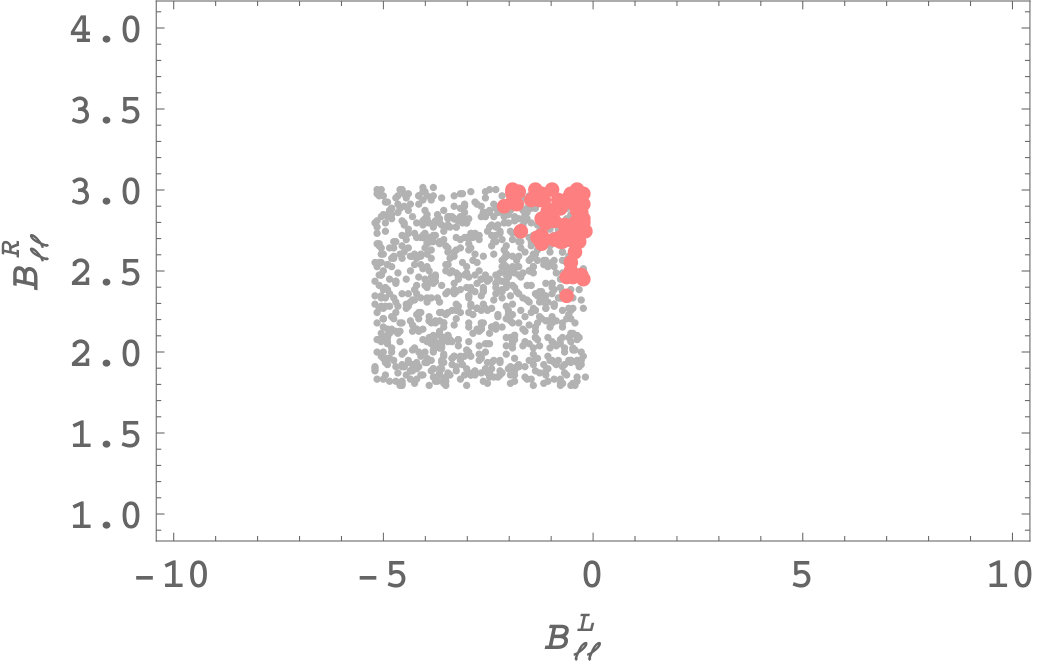 Figure 1
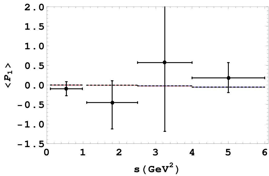 Figure 2
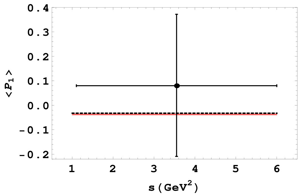 Figure 3
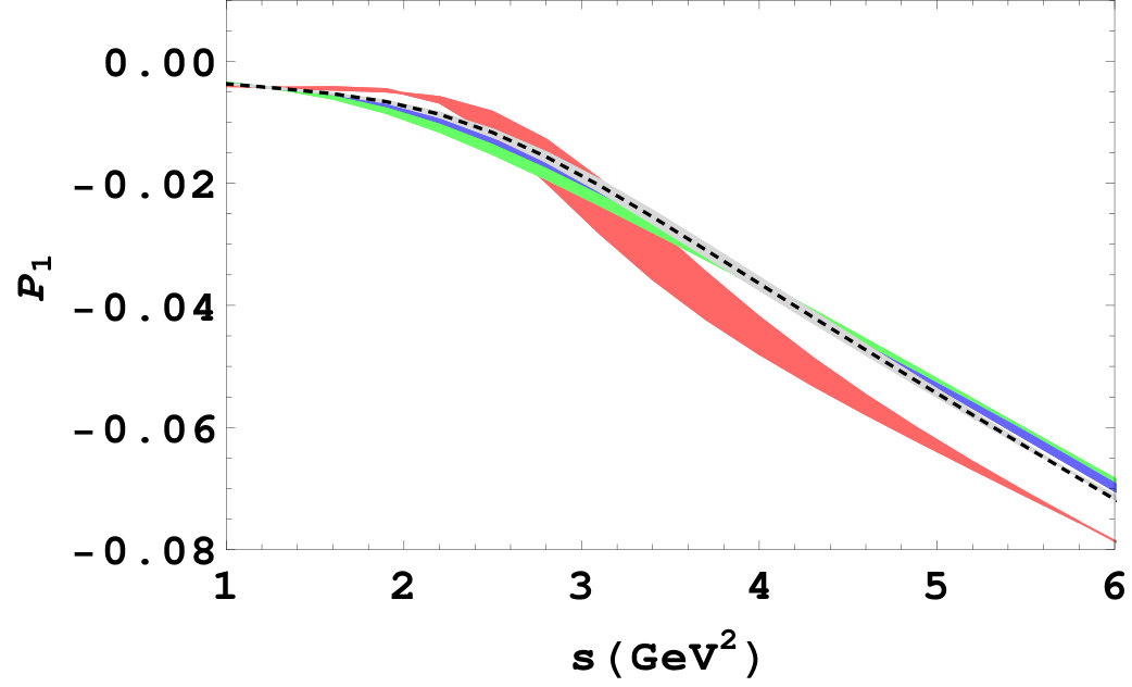 Figure 4
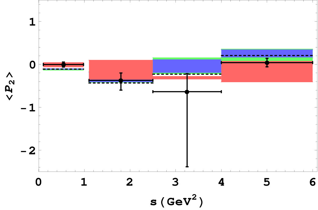 Figure 5
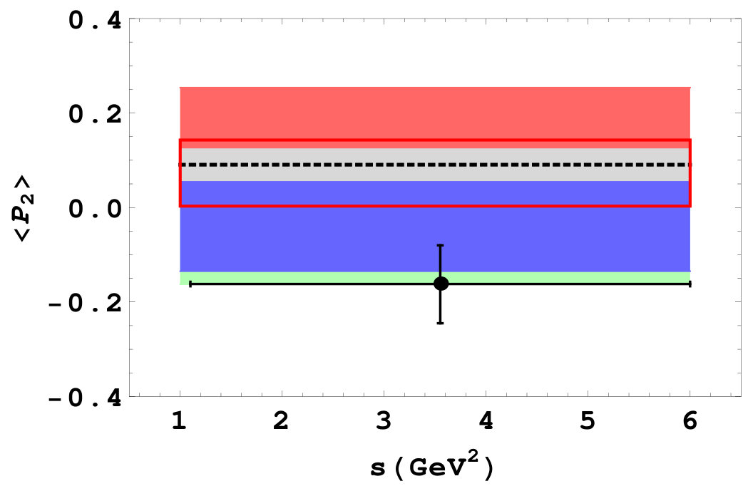 Figure 6
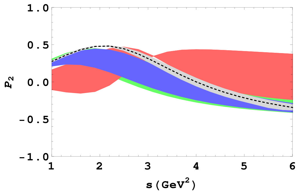 Figure 7
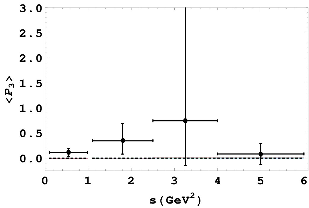 Figure 8
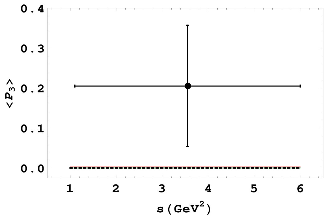 Figure 9
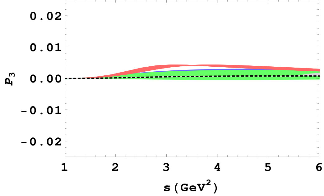 Figure 10
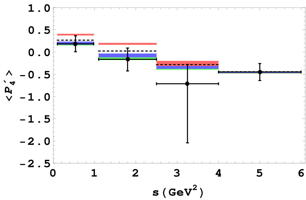 Figure 11
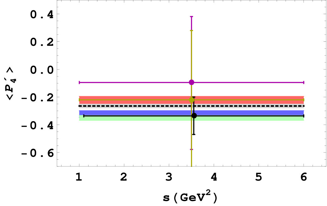 Figure 12
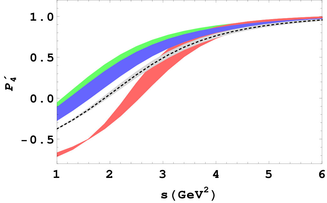 Figure 13
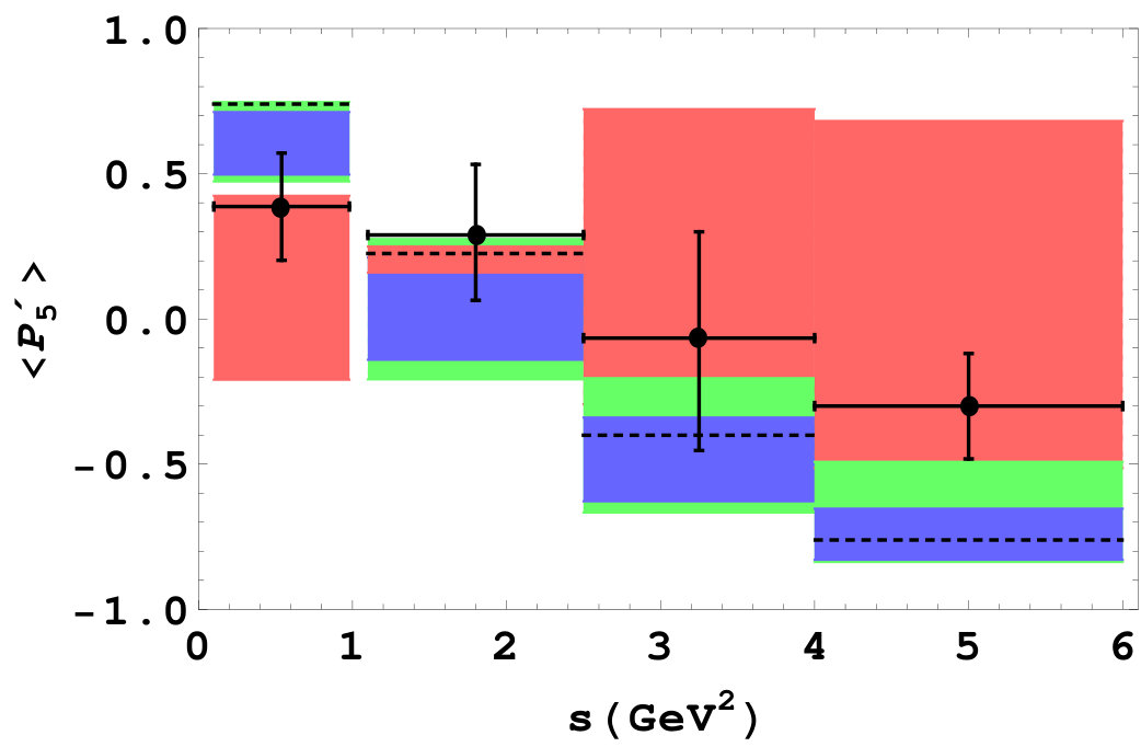 Figure 14
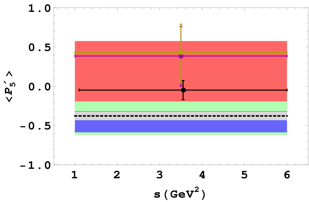 Figure 15
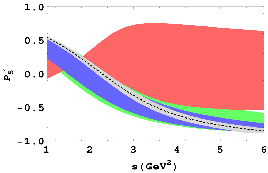 Figure 16
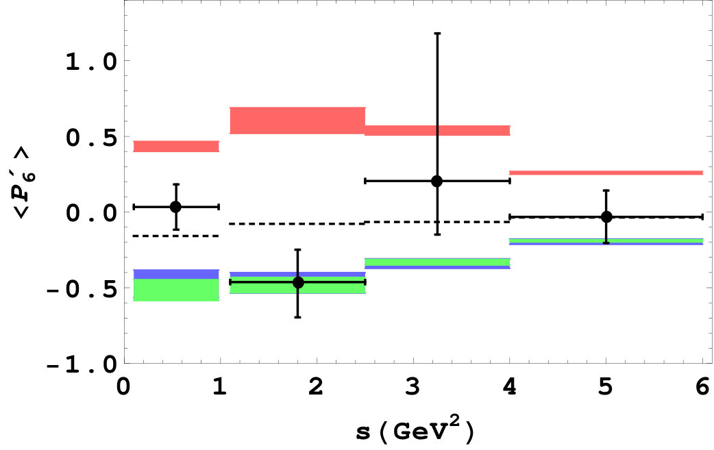 Figure 17
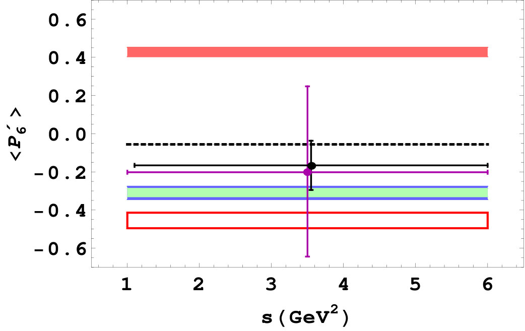 Figure 18
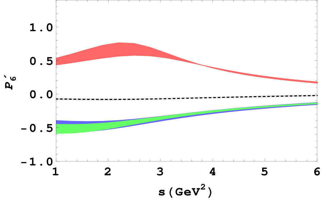 Figure 19
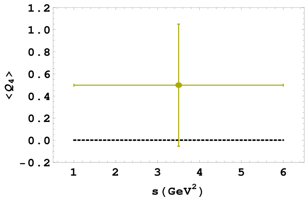 Figure 20
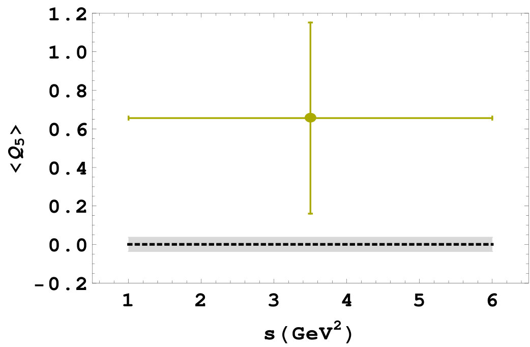 Figure 21
| 0.923 | -0.511 | 28.30 | 49.40 | |
| 0.290 | 40.38 | |||
| -0.084 | 0.342 | 52.00 |
| Obs. | SM Prediction | Measurement 2015lhcb | |||
|---|---|---|---|---|---|
| GeV2 | |||||
| GeV2 | |||||
| GeV2 | |||||
| -0.023 | |||||
| 0.001 | |||||
| GeV2 | |||||
| -0.055 | |||||
| -0.2632 | 1.0111 | -0.0055 | -0.0806 | 0.0004 | 0.0009 | -0.2923 | -0.1663 | 4.0749 | -4.3085 |
| or |
Peer Reviews
No public reviews on file for this paper yet. If you reviewed it on a platform where reviews are public (OpenReview, ICLR, NeurIPS, ICML), you can paste yours below so the community can read it here.
Videos
No videos yet. Explain this paper in a talk, walkthrough, or lecture? Add one.
LHCb anomaly in optimised
observables and potential of Model
Ishtiaq Ahmed[email protected], Abdur Rehman[email protected]
1National Centre for Physics, Quaid-i-Azam University Campus, Islamabad, 45320 Pakistan
Abstract
Over the last few years LHCb with present energies found some discrepancies in FCNC transitions including anomalies in the angular observables of , particularly in , in low dimuon mass region. Recently, these anomalies are confirmed by Belle, CMS and ATLAS. As the direct evidence of physics beyond-the-SM is absent so far, therefore, these anomalies are being interpreted as indirect hint of new physics. In this context, we study the implication of non universal family of model to the angular observables , and newly proposed lepton flavor universality violation observables, , in decay channel in the low dimuon mass region. To see variation in the values of these observables from their standard model values, we have chosen the different scenarios of the model. It is found that these angular observables are sensitive to the values of the parameters of model. We have also found that with the present parametric space of model, the -anomaly could be accommodated. However, more statistics on the anomalies in the angular observables are helpful to reveal the status of the considered model and, in general, the nature of new physics.
pacs:
13.20 He, 14.40 Nd
I Introduction
In flavor physics, the study of rare meson decays provide us a powerful tool, not only to test the standard model (SM) at loop level but also to search the possible new physics (NP). searching of NP in rare decays of B-meson demands to focus on those observables which contain minimum hadronic uncertainties such that they can be predicted precisely in the SM and are available at current colliders. In exclusive rare B meson decays, the main source of hadronic uncertainties come from the form factors which are non-perturbative quantities and are difficult to compute. In addition, these uncertainties may preclude the signature of any possible NP. From this point of view, among all rare decays, the four body decay channel, , have a special interest in literature due to the fact that it gives a large variety of angular observables, namely, and DescotesGenon:2012zf which are free from hadronic uncertainties Descotes-Genon:2013vna . The comparison between the theoretical predictions of these kind of observables in the SM with the experimental data could be helpful to clear some smog on the physics beyond the SM.
From experimental point of view, few years back, LHCb measured the values of these angular observables for the decay channel . These measurements found a 3.7 deviation in the value of , with 1 fb*-1* luminosity in the GeV2 bin 2013lhcb . Recently, this discrepancy again seen at LHCb with a 3 deviation with 3 fb*-1* luminosity in comparatively two shorter adjacent bins GeV2 2015lhcb and GeV2 which is also confirmed by Belle in the larger bin GeV2 belle2016 ; Wehle:2016yoi . The very recent results from ATLAS ATLAS-CONF-2017-023 and CMS CMS-PAS-BPH-15-008 ; Khachatryan:2015isa collaborations, presented in Moriond 2017, are also confirmed this discrepancy. Furthermore, LHCb also found 2.6 deviation in the value of BrBr rk , and \mathrel{\raise 1.29167pt\hbox{>\kern-7.5pt\lower 4.30554pt\hbox{\sim}}}2\sigma in the Br lhcbphi . Interestingly, all these deviations belong to the flavor changing neutral current (FCNC) transitions, , where denotes the final state leptons.
The anomalies, mentioned above, are slowly piled up and received a considerable attention in the literature (see for instance Matias:2012xw ; Altmannshofer:2017fio ). It is also important to mention here that even the angular observables are form factor independent (FFI) but for precise theoretical predictions, one needs to incorporate the factorizable and non-factorizable QCD corrections. The factorizable corrections absorb in the hadronic form factors while the non-factorizable corrections arise from hard scattering of the process and do not belong to the form factors. In this respect, there are some studies which focus to the question whether these anomalies emerge from unknown factorizable power corrections or from NP Capdevila:2017ert ; Chobanova:2017ghn . However, global fit analysis with present data, strongly pointed out that the interpretation of mentioned anomalies through the NP is a valid option Altmannshofer:2017fio . In the present study, to determine the values of angular observables, we have included both type of corrections up to next-to-leading order (NLO) and their expressions are given in Appendix B.
From NP point of view, several extensions of the SM have been put forwarded models ; Egede:2010zc ; Altmannshofer14 ; bobeth13 ; thurth14 ; jager14 ; Allanach:2015gkd ; Crivellin:2015era ; Jager:2017gal . Among these, the model is economical due to the fact that besides the SM gauge group, it requires only one extra gauge symmetry associated with a neutral gauge boson, called . The nature of couplings of the boson with the quarks and leptons leads the FCNC transitions to the tree level. In this model, the NP effects comes only through the short distance Wilson coefficients which are encapsulated in the new coefficients , , while operator basis remained unchange.
Several previous studies shown a possible interpretation to alleviate the mismatch between the experimental data of different observables for the decay and their SM predictions in terms of model Descotes-Genon:2013wba ; Altmannshofer:2013foa ; Gauld:2013qba ; Gauld:2013qja ; Buras:2013dea ; Buras:2013qja without any conflict. Therefore, it is natural to ask whether the model could explain the recently observed anomalies in the angular observables of the decay channel . With this motivation, in the current study, we have analyzed the optimal observables and , in the low dimuon mass region, for the in the SM and in the model. Besides these observables, we have also calculated the violation of lepton flavor universality (LFU) observables namely, Capdevila:2016ivx . For numerical calculations of these observables, we have used the LCSR values of the hadronic form factors zwicky05 and for parameters, we have used the Utfit collaboration values, called as , and another different scenario, called which numerical values are listed in Tab. (5).
We would like to mention here that the considered scenarios labeled as , and have same coupling structure of the boson with the quarks and the leptons. However, the underlying difference between these scenarios is related to the different fit values of parameters such as new weak phase and couplings of model, for considered decay process, available in the literature. For example, by using the all available experimental data on mixing, Utfit collaboration has found two solutions of new weak phase, , that arises due to the measurement ambiguities in the data and referred as and . Similarly, another possible constraint on parameters of model is discussed in newcon4 that, hereafter, we label as .
This paper is organized as follows: Section II.1, contains the effective Hamiltonian for the transition in the SM and in the model. The matrix elements in terms of form factors and the expression of differential decay distributions are also given in this section. Formulae for the angular observables in section II.2. In section III, we have plotted the angular observables and their average values against dimuon mass and we have given phenomenological analysis of these observables. In the last section we conclude our work. Appendix A contains the analytical expressions of the angular observables and the values of input parameters. The contributions of factorizable and non-factorizable corrections at NLO are summarized in Appendix B.
II Formulation for the Analysis
II.1 Matrix Elements and Form Factors
In the standard model, FCNC transition, , occurs at loop level which amplitude can be written as,
[TABLE]
where , and are momentum and polarization of meson, respectively, while is the momentum of meson.
In the presence of the FCNC transitions could occur at tree level and the Hamiltion can be written in the following form (see detail in the refs. PL1 ; QCh ; KCh1 ; VB3 )
[TABLE]
The is the coupling of with quarks and , are left and right-handed couplings fo with leptons. One can notice from Eq. (II.1) that in the model, operator basis remains the same as in the SM while Wilson coefficients, and , get modified. The total amplitude for the decay is the sum of SM and contributions, and can be written as follows,
[TABLE]
where and .
The matrix elements for transition, appears in Eq. (4), can be written in terms of form factors as follows
[TABLE]
[TABLE]
where,
[TABLE]
Here , , are the form factors and contain hadronic uncertainties. At leading order by using the heavy quark limit, the QCD form factors follow the symmetry relations and can be expressed in terms of two universal form factors and hiller2 ; Beneke:2000wa .
[TABLE]
It is also important to mention here that the angular observables are soft form factor independent at LO in (i.e., not totally dependent of FF). There is residual dependence has been discussed, computed systematically and included in the predictions of the main papers of the field and even if, as expeted, does not play an important role induce certain mild dependence on FF. In addition, for the dependence of the universal form factors there are different parametrization Straub:2015ica , however, we have analyzed that the choice of parametrization is not so important at low . In the current study, we use the following parametrization of LCSR approach zwicky05 .
[TABLE]
where the parameters , and are listed in Tab. (1). The uncertainty in the universal form factors and arises from the uncertainty in the different parameters using in LCSR approach which is about and , respectively, as discussed in hiller2 .
At NLO, the relations between the where () and the invariant amplitudes , where , read as Beneke:2001at .
[TABLE]
where is the energy of kaon in the rest frame of -meson and are defined in Eq. (23) of Appendix B.
The four-fold differential decay distribution for the cascade decay is completely described by the four independent kinematical variables: the three angles; is the angle between the and mesons in the rest frame of , is the angle between lepton and meson in the dilepton rest frame while is the azimuthal angle between the dilepton rest frame and rest frame and the fourth variable is dilepton invariant squared mass . The explicit dependence of differential decay distribution on these kinematical variables can be expressed as follows
[TABLE]
where
[TABLE]
The full physical region phase space of kinematical variables is given by
[TABLE]
where , , are the masses of meson, meson and lepton, respectively.
The expressions of coefficients for and as a function of the dilepton mass , are given in Appendix A in Eq. (16). As we do not take the scalar contribution in this study, therefore, .
II.2 Expressions of the Angular Observables
The definitions of FFI angular observables (optimal observables) are given in ref. Matias:2012xw ,
[TABLE]
The primed observables (related to the ()) which are simpler and more efficient to fit experimentally are defined as,
[TABLE]
III Results and Discussion
In this section, we will present the numerical analysis of the angular observables. The authors would like to mention here that all of the numerical results are taken from the self-written Mathematica code. Before the analysis, we would like to write the different definitions of angular observables that are opted by LHCb 2015lhcb and theoretically used in the literature,
[TABLE]
For the numerical analysis the values of LCSR form factors, and relevant fit parameters are listed in Tab. (1). The values of Wilson coefficients and other input parameters are listed in Appendix A in Tabs. (4) and (6), respectively. Regarding the coupling parameters of with quarks and leptons, there are some severe constraints come from different inclusive and exclusive meson channels ConstrainedZPC1 . Particularly, coming from the two different fitting values for mixing data by the UTFit collaborationUTfit . In this study, we call these two fitting values as and and their numerical values are listed in Tab.(5). We have considered another scenario which denoted by in the present study that are obtained from the analysis of newcon1a , newcon1 ; newcon2 and newcon3 . The numerical values of scenario are chosen from cpv5 ; newcon4 and also listed in the Tab. (5). The purpose of the following analysis is to check that these constrained of parameters could accomodate the anomalies in the angular observables, particularly, in .
III.1 -observables in different bin size
The numerical values of angular observables in different low bins in SM and in , and are given in Tab. (2). For comparison with experimental measurements, the maximum likelihood fit results of LHCb 2015lhcb are also given in the table. The ranges in the values of angular observables in , and is found by setting the upper and lower values of parametric space of these scenarios. These results are also shown graphically in Figs. (1) and (2) where black crosses are the data points taken from the last column of Tab. (2) and black dashed line correspond to the SM while green, red and blue bands correspond to the , and scenarios of the model, respectively. The upper curve of the band corresponds the upper values of parametric space while the lower curve of the band corresponds the lower values of parametric space of the scenario. In our different bin sized analysis, we have not included the preliminary results from Belle belle2016 ; Wehle:2016yoi , ATLAS ATLAS-CONF-2017-023 and CMS333see figure 6 of Altmannshofer:2017fio for the recent analysis with these new results.CMS-PAS-BPH-15-008 ; Khachatryan:2015isa because their bin intervals are different from LHCb 2015lhcb that we have discussed in this section. In Fig. (1), the gray shaded region corresponds to the uncertainty in the SM values due to the uncertainty in different input parameters. One can see from the left panel of Figs. (1) and (2) that the uncertainty band in SM not preclude the effects of model. Therefore, we have not provided the SM uncertainty in Tab. (2) and hence in the right panel of Figs. (1) and (2).
The plots in first and third rows of Fig. (1), represent the variation in the values of and their average values as a function of in the SM and in the different scenarios of model. From these graphs one can see that the values of these observables are quite small in the SM and not much enhanced when we incorporate the effects. One can also see from Fig. (1) that the SM values of lie inside the measured values. As the error in the measurement is huge, therefore, no potent result can be drawn from this observable with the current data. On the other hand the values of in last two bins are within the measured values while in first two bins the SM values are out of the measured bars. However, to say something about any discrepancy in these observables, reduction in the experimental uncertainties are required.
Plots in second row of Fig. (1), show the variation in the values of and its average against dilepton mass . It could be seen from these figures that the values of these observables are significantly influenced in the presence of effects. The right plot in the second row of Fig. (1) shows that the SM values of in the bins and lie within the measurements and also in the bin when the theoretical uncertainties of the input parameters are taken into account. However, in the first bin , the SM value of looks mismatch from the experimental value. But it is worthy to mention here that the measurement performed by LHCb in this bin is without including the suppressed terms which are important at very low region and it was found in Descotes-Genon:2015uva , that the impact of these terms is about reduction in the value of . Regarding this, it is mentioned in Capdevila:2017ert that in the first bin, LHCb actually measured instead of . Therefore, in principle, one could say that, up-till now, there is no mismatch between the SM predicted values of with the experimental values.
In the first row of Fig. (2), we have displayed and it’s average value, , in the SM and in the different scenarios of model as a function of . One can see from these plots that the effects are quite significant in the values at low region but mild at larger values of . However, the SM values of in all four bins lie inside the measured values.
The results of and it’s average value in the SM and in the models are presented in the second row of Figs. (2). The values are significantly changed from the SM values when we incorporate the effects. It can be noticed in the bin GeV2, the SM average value mismatch with the experimental values and as mentioned in the introduction that LHCb found 3 deviation in this bin. It could be seen from the figure that this discrepancy can be alleviated by (red band) of model. On the other hand for the Utfit scenarios, namely, and it can be noticed that when we take the upper and lower limit values of the current parametric space of these scenarios (green and blue bands), the anomaly in the bin GeV2 can not be accommodated. However, if the values of different parameters are chosen randomly within the allowed range then one could accommodate the anomaly in this bin by but not with . Therefore, it looks that the of Utfit is not consistent with the present data while the parametric space of , the left (right) couplings, (, ), of with leptons is severely constraint as shown in Fig. (3).
In the third row of Fig. (2), we have shown the variation of and as a function of . Similar to , the SM value of this observable is also suppressed. As seen from the graph that SM value of consistent with the data with large error bars, however there is 2 deviation in one bin which probably will be disappear when data will increase. One can also notice that in contrast to the , the value of significantly enhanced in the model. It is also noticed that in the model the value of is positive in scenarios and while becomes negative in . As for the present analysis in , we set the value of , in contrast to this, if we choose which is also allowed (see Tab. (V)), then this negative value becomes positive.
III.2 -observables in GeV2
Besides the analysis of angular observables in shorter bins at low region (discussed in previous section), we have also analyzed these observables in the full GeV2 region. The results for -observables in GeV2 are summarized in Tab. (3) and corresponding plots are shown in Fig. (4). In this figure, black error bar corresponds to LHCb result 2015lhcb while, magenta and yellow error bars correspond to Belle measurements for some of these observables belle2016 ; Wehle:2016yoi . However, it is good to mention here that LHCb results are in the bin GeV2 while Belle measurements belle2016 ; Wehle:2016yoi are in the GeV2. In addition, recently, the ATLAS collaboration announced its results for GeV2 ATLAS-CONF-2017-023 which is not included in the current analysis. The empty red boxes in the plots of and represent the scenario when we choose , while, other legends are same as in Figs. (1) and (2).
From Fig. (4), one can immediately notice that the values of and in the SM and in all the three scenarios of lie within the current measurements, however, the error bars are huge. Therefore, to extract any information about the NP requires the precise measurement of these observables. It is also noticed that the values of in the SM and in the scenarios are very close, consequently, this observable even after the reduction of error bars not a good candidate to constrained the parametric space. On the other hand could be helpful to constraint the parametric space, if any mismatch will appear in future in the bin [1,6] GeV2. The SM value of is small and not enhanced in model. However, the measured value is well above the SM prediction with huge error bars and need precision to draw any conclusion from this observable as well. From graph of in Fig. (4), one can deduced that the SM value of not lie within the measured value of LHCb. However, the values of in and are within the measurements while in , the value is out side the measured error bars. For , we have two different measurements as shown in the plot and contrast to the , the value of lie within these measurements. However, similar to the values of in and lie within the measurements while the value in lies outside the measured values (see red bands in both plots). Regarding , it is interesting to check whether the values of and could be reduced to current measurements. For this purpose, we choose the weak phase with opposite sign i.e., (see Tab. 5 in Appendix A) and represent them in plots by empty red boxes. In Fig. 4, by looking the empty red box in plot, the value is reduced but still well above the current measurement. In contrast, the value of reduce to the Belle measurements belle2016 . However, more statistics on the observables and are helpful to constrained the parameters, particularly, the sign and the magnitude of new weak phase .
For plots of Fig. (3), the values in the SM and in , lie out side the error bars of experimental data points while the values in the well inside the all data points shown in figure. In general, from the plots of Fig. (3), one concludes that the considered model do have potential to remove mismatch between theory and experiment but it is not so conclusive at present. We hope more precise measurements will clear the situation.
III.3 for GeV2
In Fig. (5), we have plotted the lepton flavor universality violation (LFUV) observables against . The values are quite small in the SM approximately in the bin GeV2. We have also found that the effects of are negligible. This fact is trivial, since Eq. (3) implies . However, error bars are quite large and need more experimental data to find the accurate values of these observables.
IV Conclusion
In the present study, we have calculated the angular observables and their average values in the SM and in the noun-universal family of model for the decay channel . The expressions of the angular observables are given in the form of coefficient which are written in terms of auxiliary functions in Eq. (16). As in the literature, these coefficients, in general, expressed via transversity amplitudes, , and , so the relations of these transversity amplitudes with auxiliary function are also given in Eq. (LABEL:TARelation). To see the effects on these observables, we have used the UtFit collaboration constraints for the parameters, called as scenarios and . Besides, we also consider another scenario, called , in the present study. From the present analysis, in all three scenarios of for small values of i.e the large recoil region, the values of angular observables are significantly changed from their SM values. The current analysis shown that except the sceanario , the scenarios and of model has potential to accommodate the mismatch between the recent experimental measurements and the SM values of some of the angular observables in some bins of . For instance, there is a discrepancy between experimentally measured value and SM value of in the region GeV2 and in the current study it is found that scenario of could be adjusted this mismatch value with the measured value in this bin. On the other hand, this mismatch can not be accommodated on taking the maximum and minimum values of different parameters of scenarios and of UtFit collaborations. However, when we choose the random values of different parameters in the allowed region of these scenarios, one can accommodate the anomaly with scenario but not with scenario . It is also noticed that the anomaly further constraint on the allowed parametric space of . Furthermore, we have also calculated the angular observables and the LFUV observables in the large bin and plotted with the measured data, however, the error bar is quite large in this bin and more static is needed to draw results. Here, we would like to comment that CMS and ATLAS collaborations recently announced preliminary results on angular observables in Moriond 2017 which still show the tension between experimental measurements and the SM predictions. Therefore, in general, one can say, as data will be enlarge and the statistical error will be reduced then these observables are quite promising to say something about the constraints on coupling of boson with the quarks and leptons and consequently about the status of model.
Appendix A
The expressions of appeared in Eqs. (13) and (14) are as follows,
[TABLE]
[TABLE]
[TABLE]
where (), are the auxiliary functions and given as follows,
[TABLE]
[TABLE]
and a where is given in Appendix B in Eq. (LABEL:delta).
Traditionally, the ’s are given in terms of transversity amplitudes but we have written in terms of functions given in Eq. (17) . The are related with as follows
[TABLE]
where . We would like to mention here that our expressions of ’s are consistent with the literature for example given in refs. Matias:2012xw ; ball .
The values of Wilson coefficients at NNLO, parameters and other input parameters are listed in Tabs. (4), (5) and (6), respectively.
Appendix B
The expression of , appear in the definition of a0 below Eq. (18), written as follows
[TABLE]
and contributes only for massive leptons. The light-cone distribution amplitude (LCDA) for transversely and longitudinally polarized can be written as Beneke:2001at ; ball03
[TABLE]
where and are the Gegenbauer coefficients. The moments are
[TABLE]
where are the two -meson light-cone distribution amplitudes Beneke:2001at . The can be expressed as:
[TABLE]
where . The are the universal form factors,
[TABLE]
The matrix elements in heavy quark limit depend on four independent functions . In the low , (GeV2), the invariant amplitudes at NLO within QCDf are given in hiller2 ; ball ; Beneke:2001at ,
[TABLE]
where , and the factorization scale . The coefficient functions and hard scattering functions are written as
[TABLE]
The form factor terms at LO are
[TABLE]
[TABLE]
where is well-known fermionic loop function.
The coefficients at NLO is divided into a factorizable and a non-factorizable part as
[TABLE]
At NLO the factorizable correction reads Beneke:2001at ; beneke05
[TABLE]
The non-factorizable corrections are,
[TABLE]
where depends on the mass renormalization convention for . These corrections are obtained from the matrix elements of four-quark and chromomagnetic dipole operators Beneke:2001at that are embedded in and asatryan01 ; greub08 .
At LO the hard-spectator scattering term from weak annihilation diagram is Beneke:2001at
[TABLE]
[TABLE]
The contributions to at NLO also contain a factorizable as well as non-factorizable part
[TABLE]
Including corrections the factorizable term to are given by Beneke:2001at ; beneke05
[TABLE]
where . The non-factorizable correction comes through the matrix elements of four-quark operators and the chromomagnetic dipole operator
[TABLE]
The functions are given by
[TABLE]
where and are
[TABLE]
[TABLE]
and
[TABLE]
[TABLE]
The reference list from the paper itself. Each links out to its DOI / PubMed record.
- 1(1) S. Descotes-Genon, J. Matias, M. Ramon and J. Virto, JHEP 1301 , 048 (2013) doi:10.1007/JHEP 01(2013)048 [ar Xiv:1207.2753 [hep-ph]].
- 2(2) S. Descotes-Genon, T. Hurth, J. Matias and J. Virto, “Optimizing the basis of B → K ∗ l l → 𝐵 𝐾 𝑙 𝑙 B\to K*ll observables in the full kinematic range,” JHEP 1305 , 137 (2013), [ar Xiv:1303.5794 [hep-ph]].
- 3(3) LH Cb Collaboration, “Measurement of Form-Factor-Independent Observables in the Decay B 0 → K ∗ 0 μ + μ − → superscript 𝐵 0 superscript 𝐾 absent 0 superscript 𝜇 superscript 𝜇 B^{0}\to K^{*0}\mu^{+}\mu^{-} ,” PRL 111 (2013) 191801 [ar Xiv:1308.1707 [hep-ex]].
- 4(4) R. Aaij et al. [LH Cb Collaboration], “Angular analysis of the B 0 → K ∗ 0 μ + μ − → superscript 𝐵 0 superscript 𝐾 absent 0 superscript 𝜇 superscript 𝜇 B^{0}\to K^{*0}\mu^{+}\mu^{-} decay using 3 fb -1 of integrated luminosity,” JHEP 1602 (2016) 104 [ar Xiv:1512.04442 [hep-ex]].
- 5(5) A. Bharucha, D. M. Straub and R. Zwicky, JHEP 1608 , 098 (2016) doi:10.1007/JHEP 08(2016)098 [ar Xiv:1503.05534 [hep-ph]].
- 6(6) A. Abdesselam et al. [Belle Collaboration], “Angular analysis of B 0 → K ∗ ( 892 ) 0 ℓ + ℓ − → superscript 𝐵 0 superscript 𝐾 ∗ superscript 892 0 superscript ℓ superscript ℓ B^{0}\to K^{\ast}(892)^{0}\ell^{+}\ell^{-} ,” ar Xiv:1604.04042 [hep-ex].
- 7(7) S. Wehle et al. [Belle Collaboration], “Lepton-Flavor-Dependent Angular Analysis of B → K ∗ ℓ + ℓ − → 𝐵 superscript 𝐾 ∗ superscript ℓ superscript ℓ B\to K^{\ast}\ell^{+}\ell^{-} ,” ar Xiv:1612.05014 [hep-ex].
- 8(8) ATLAS Collaboration, Angular analysis of B d 0 → K ∗ μ + μ − → subscript superscript 𝐵 0 𝑑 superscript 𝐾 superscript 𝜇 superscript 𝜇 B^{0}_{d}\to K^{*}\mu^{+}\mu^{-} decays in p p 𝑝 𝑝 pp collisions at s = 8 𝑠 8 \sqrt{s}=8 Te V with the ATLAS detector , Tech. Rep. ATLAS-CONF-2017-023, CERN, Geneva, 2017.