Stepsize-adaptive integrators for dissipative solitons in cubic-quintic complex Ginzburg-Landau equations
X. Ding, S. H. Kang

TL;DR
This survey evaluates adaptive exponential integrators for solving stiff cubic-quintic complex Ginzburg-Landau equations, focusing on accuracy near pulsating and exploding solitons with multiple time scales.
Contribution
It introduces and compares stepsize-adaptive exponential integrator schemes, including new formulas and a comoving frame approach for improved performance.
Findings
Adaptive integrators effectively handle multiple time scales.
The comoving frame improves phase rotation resolution.
Thorough numerical comparisons demonstrate method strengths.
Abstract
This paper is a survey on exponential integrators to solve cubic-quintic complex Ginzburg-Landau equations and related stiff problems. In particular, we are interested in accurate computation near the pulsating and exploding soliton solutions where different time scales exist. We explore stepsize-adaptive variations of three types of exponential integrators: integrating factor (IF) methods, exponential Runge-Kutta (ERK) methods and split-step (SS) methods, and their embedded versions for computation and comparison. We present the details, derive formulas for completeness, and consider seven different stepsize-adaptive integrating schemes to solve the cubic-quintic complex Ginzburg-Landau equation. Moreover, we propose using a comoving frame to resolve fast phase rotation for better performance. We present thorough comparisons and experiments in the one- and two-dimensional cubic-quintic…
Click any figure to enlarge with its caption.
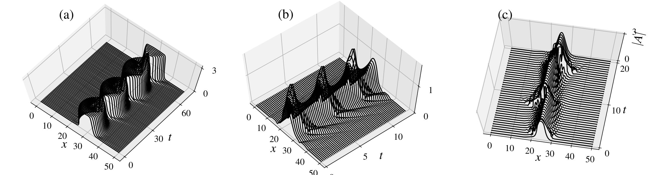 Figure 1
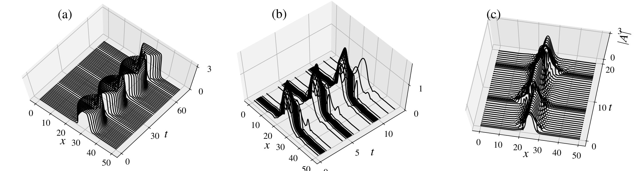 Figure 2
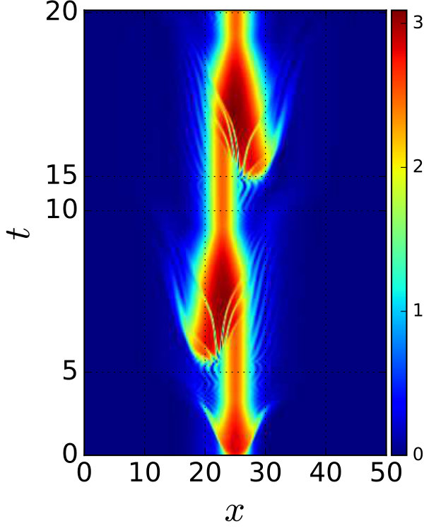 Figure 3
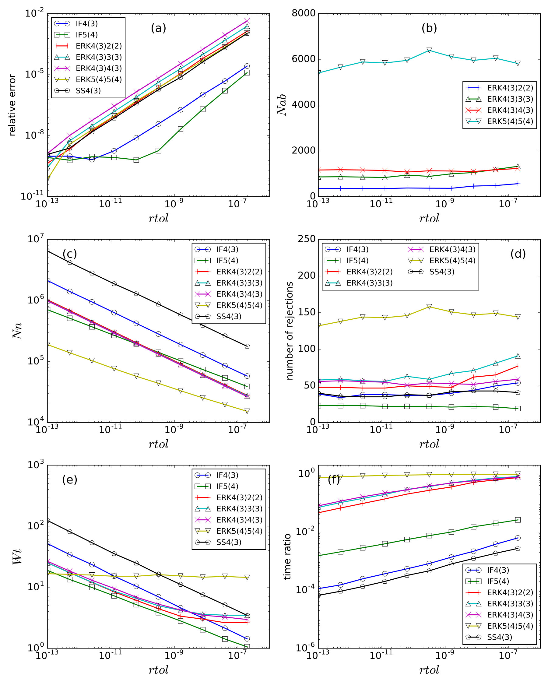 Figure 4
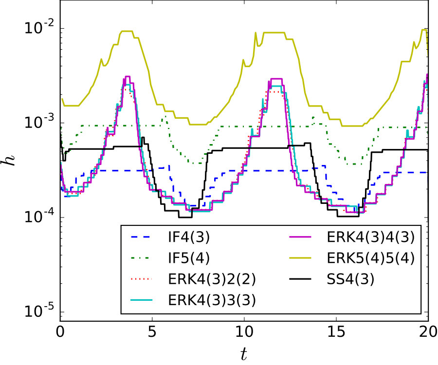 Figure 5
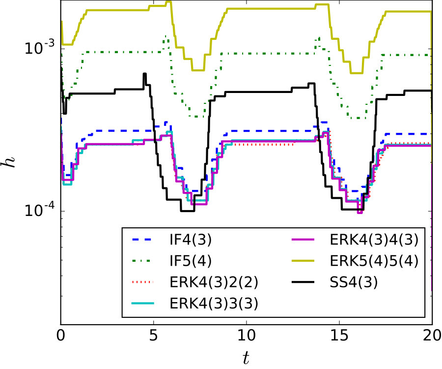 Figure 6
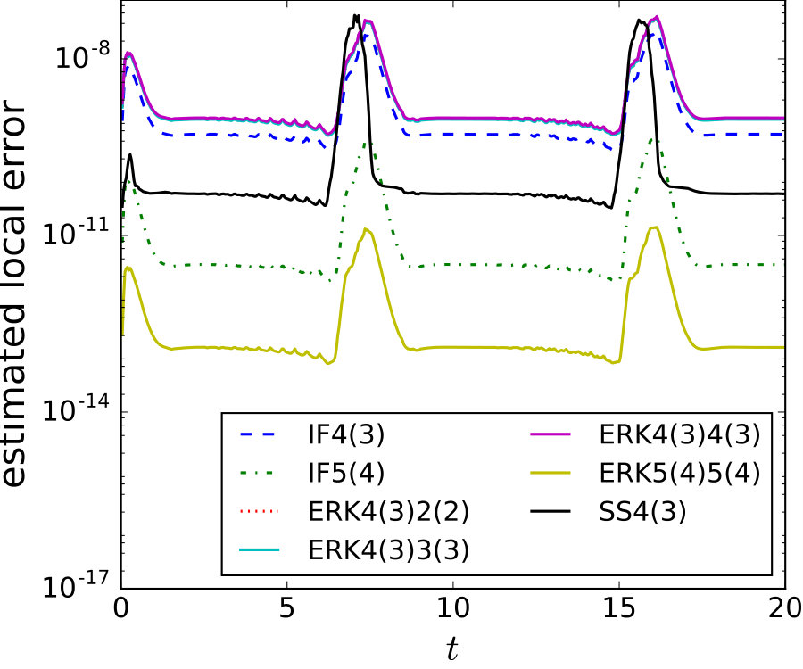 Figure 7
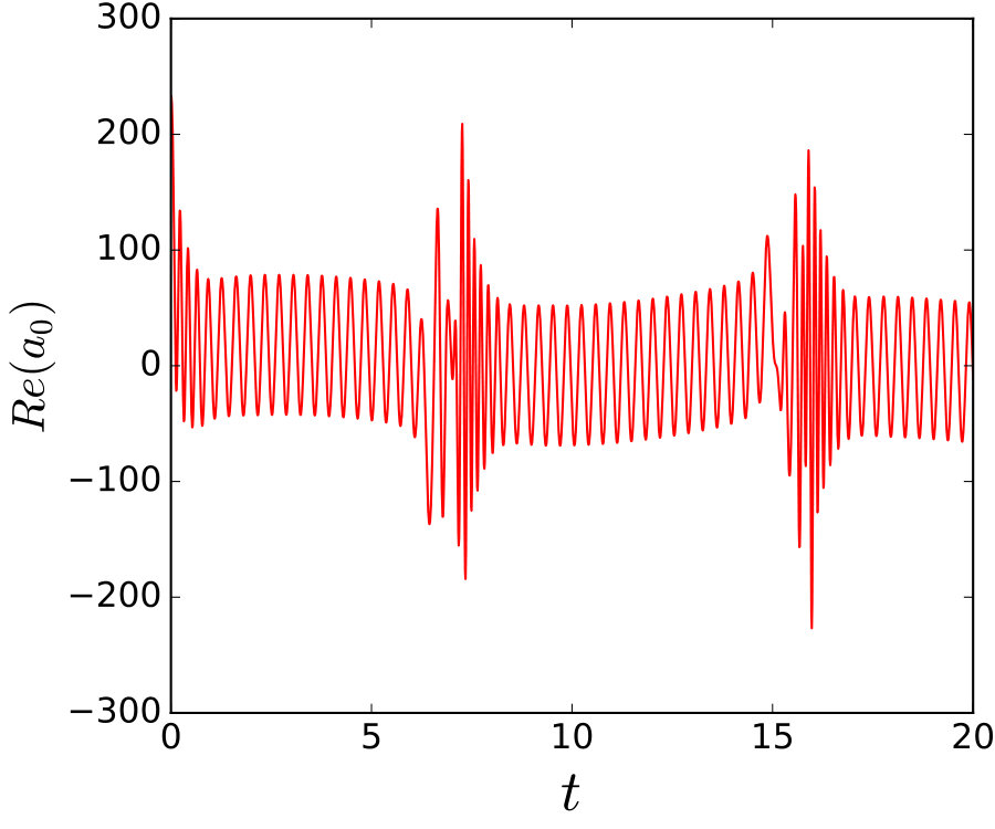 Figure 8
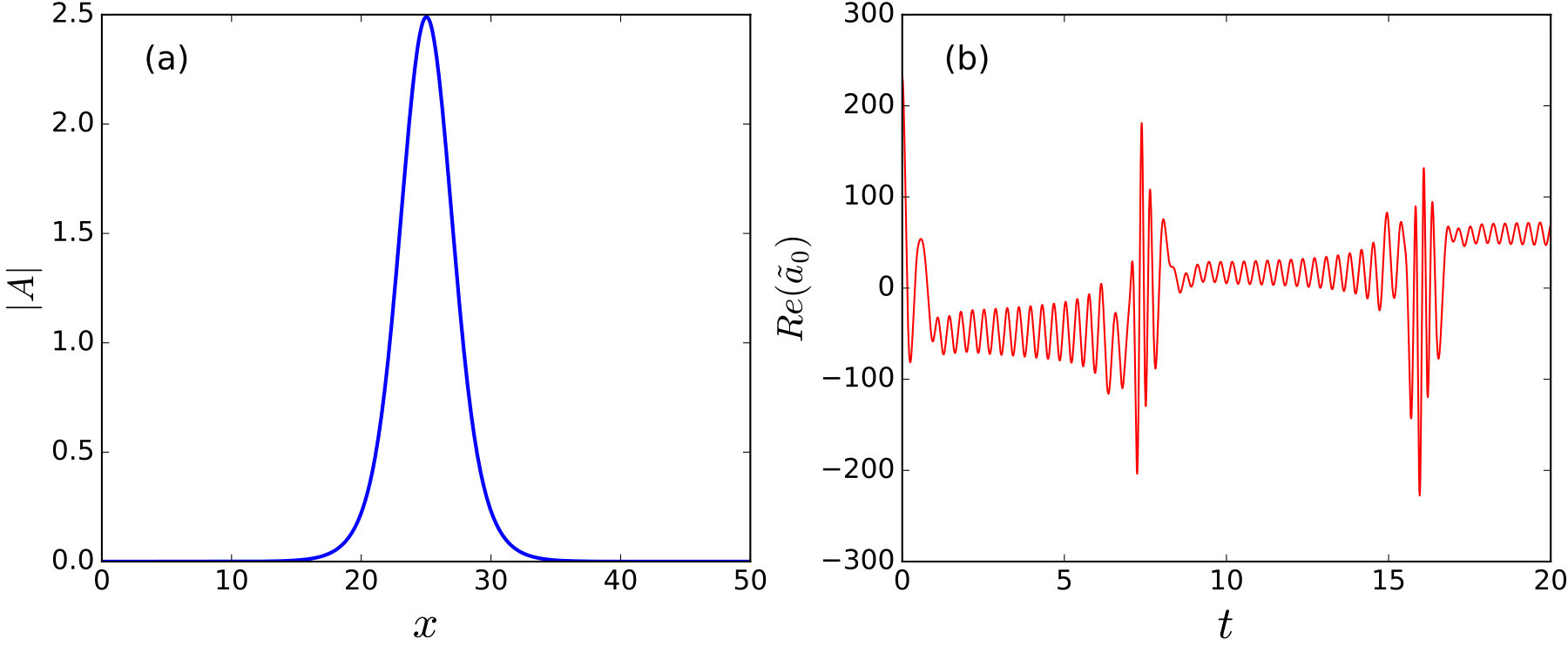 Figure 9
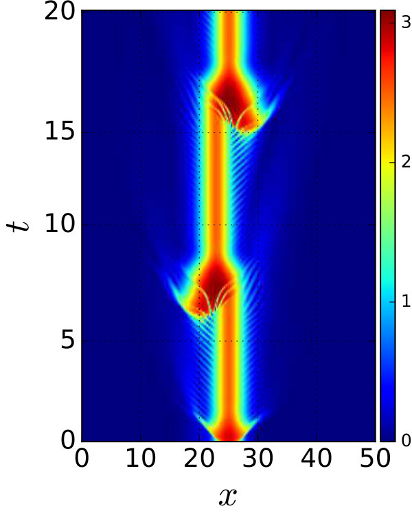 Figure 10
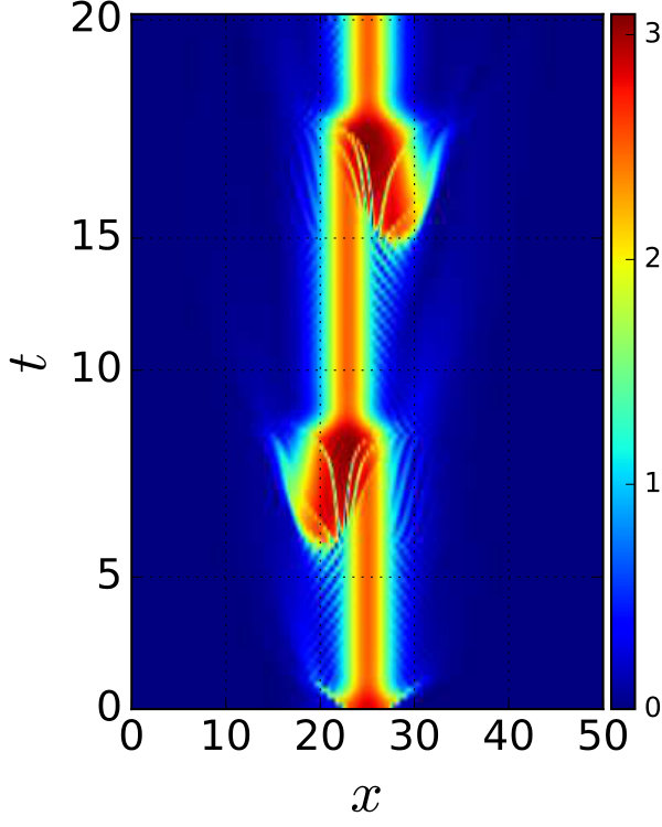 Figure 11
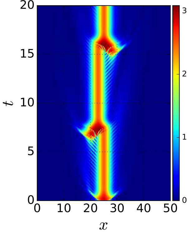 Figure 12
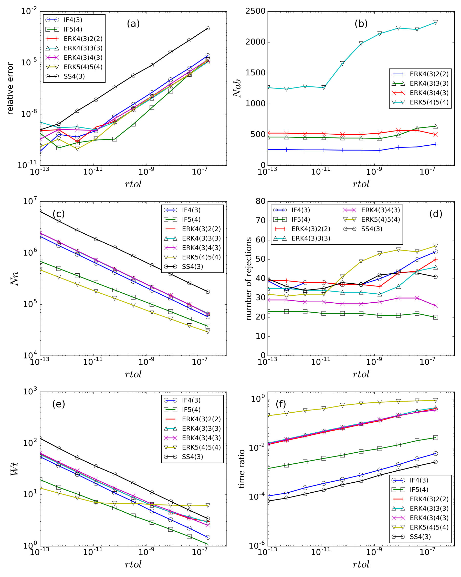 Figure 13
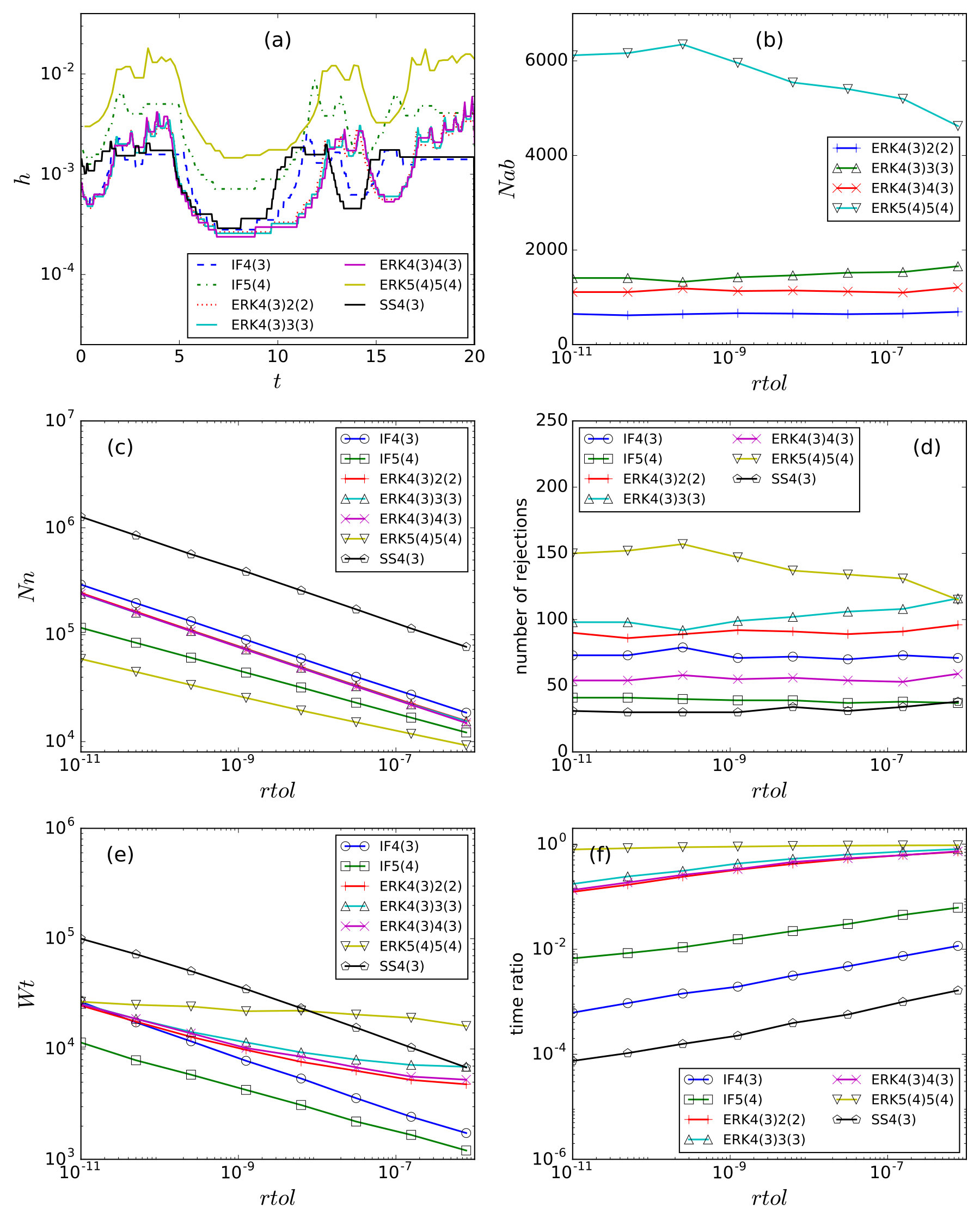 Figure 14
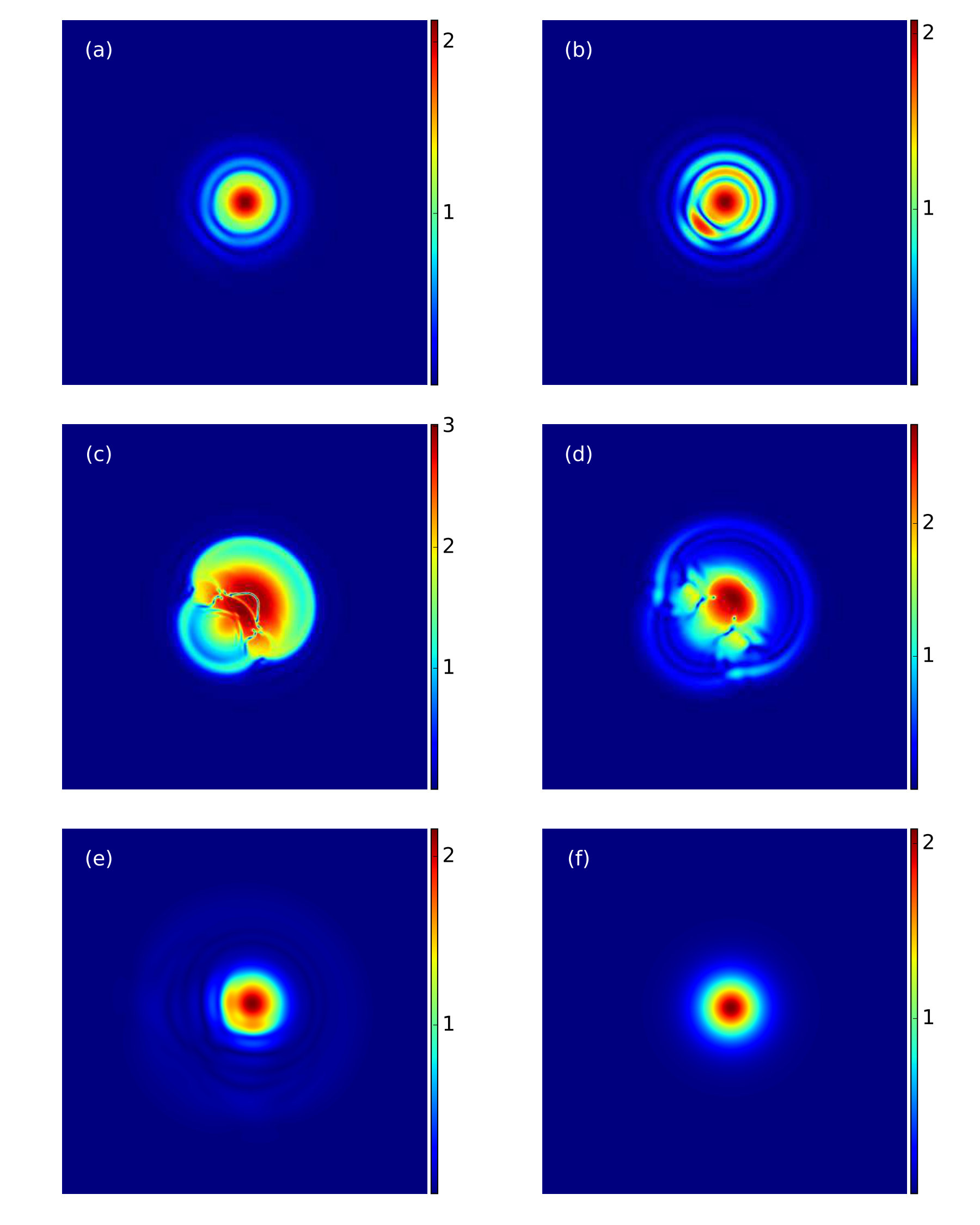 Figure 15
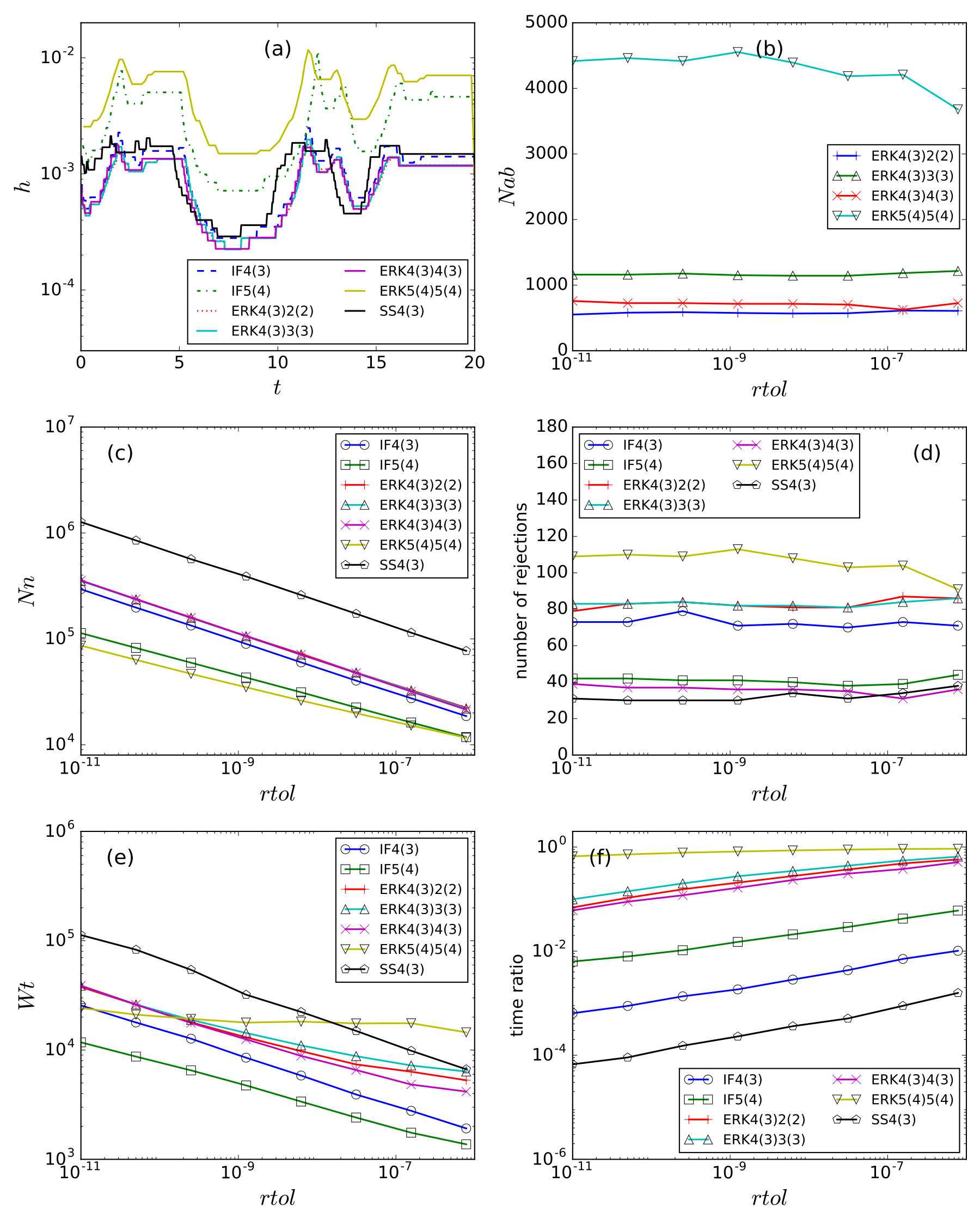 Figure 16
| Order | Index | Stiff order condition |
|---|---|---|
| 1 | 1 | |
| 2 | 2 | |
| 3 | ||
| 3 | 4 | |
| 5 |
| 0 | |||||
|---|---|---|---|---|---|
| 0 | |||||
| 1 | 0 | 0 | |||
| 1 | |||||
| 0 | |||||
|---|---|---|---|---|---|
| 0 | |||||
| 1 | 0 | ||||
| 1 | |||||
| 0 | |||||
| 0 |
| 0 | |||||
|---|---|---|---|---|---|
| 1 | 0 | ||||
| 1 | |||||
| 0 | |||||
| 0 |
| scheme | order | nn | nab | |
| IF4(3) | 4 | 5 | - | |
| IF5(4) | 5 | 7 | - | |
| ERK4(3)2(2) | 4 | 5 | 4 | |
| ERK4(3)3(3) | 4 | 5 | 8 | |
| ERK4(3)4(3) | 4 | 5 | 11 | |
| ERK5(4)5(4) | 5 | 9 | 23 | |
| SS4(3) | 4 | 24 | - |
| Tree | condition | |
|---|---|---|
| 1 | ||
| 2 | ||
| 3 | ||
| 4 | ||
| 5 | ||
| 6 | ||
| 7 | ||
| 8 | ||
| 9 | ||
| 10 | ||
| 11 | ||
| 12 | ||
| 13 | ||
| 14 |
Peer Reviews
No public reviews on file for this paper yet. If you reviewed it on a platform where reviews are public (OpenReview, ICLR, NeurIPS, ICML), you can paste yours below so the community can read it here.
Videos
No videos yet. Explain this paper in a talk, walkthrough, or lecture? Add one.
Taxonomy
TopicsNonlinear Dynamics and Pattern Formation · Numerical methods for differential equations · Advanced Fiber Laser Technologies
Stepsize-adaptive integrators for dissipative solitons in cubic-quintic complex Ginzburg-Landau equations
X. Ding
S. H. Kang
Center for Nonlinear Science, School of Physics, Georgia Institute of Technology, Atlanta, GA 30332-0430, USA
School of Mathematics, Georgia Institute of Technology, Atlanta, GA 30332-0430, USA
Abstract
This paper is a survey on exponential integrators to solve cubic-quintic complex Ginzburg-Landau equations and related stiff problems. In particular, we are interested in accurate computation near the pulsating and exploding soliton solutions where different time scales exist. We explore stepsize-adaptive variations of three types of exponential integrators: integrating factor (IF) methods, exponential Runge-Kutta (ERK) methods and split-step (SS) methods, and their embedded versions for computation and comparison. We present the details, derive formulas for completeness, and consider seven different stepsize-adaptive integrating schemes to solve the cubic-quintic complex Ginzburg-Landau equation. Moreover, we propose using a comoving frame to resolve fast phase rotation for better performance. We present thorough comparisons and experiments in the one- and two-dimensional cubic-quintic complex Ginzburg-Landau equations.
keywords:
stepsize-adaptive, cubic-quintic complex Ginzburg-Landau, dissipative solitons , exponential integrator, comoving frame
††journal: Computer Physics Communications
1 Introduction
The complex Ginzburg-Landau equation [1, 2] is one of the most frequently studied nonlinear equations in physics and applied mathematics community. Derived as a general amplitude equation near the onset of instability in the context of pattern formation [1], it has applications in various fields of physics ranging from nonlinear optics [3] to superconductivity [4]. In order to preserve the invariance of the equation under a phase change , complex Ginzburg-Landau equations only have odd-order nonlinear terms. The form with a cubic term is frequently used to study spatiotemporal chaos and intermittent traveling waves. Recently, complex Ginzburg-Landau equation with an additional quintic term
[TABLE]
has attracted attention for its peculiar dissipative soliton solutions in one- and two-dimensional cases [5, 3, 6, 7, 8, 9]. Here, or is a complex field. stands for the Laplace operator or . A dissipative soliton is a self-localized structure that arises in spatially extended dissipative systems. It maintains its shape temporally similar to a constantly propagating solitary wave packet in an optical medium. Dissipative solitons appear as a result of the balance between dispersion and nonlinearity and the balance between the gain and loss of energy. Dispersion spreads the shape while nonlinearity focuses it. A nontrivial internal energy flow and the dependence on an external energy source differentiate dissipative solitons from solitons in integrable systems. Apart from a phase shift, solitons in integrable systems remain unchanged during soliton-soliton interactions; while dissipative solitons are free from energy or momentum conservation during scattering and annihilation. For a more comprehensive discussion on dissipative solitons, see ref. [10]. While dissipative solitons lack most of the very special properties of soliton solutions of integrable Hamiltonian systems, they are generic and physically important, both because such structures are observed for wide ranges of equation parameters [11, 12], and because many types of (pulsating) soliton solutions are observed in laser experiments [13, 14, 15].
By exploring the parameter space of (1), Akhmediev et al. [3, 6] identified several types of dissipative soliton solutions, such as plain soliton, pulsating soliton, zig-zag soliton, creeping soliton, composite soliton, exploding soliton, chaotic soliton and so on, some of which are shown in figure 1. These discoveries stimulate further investigation in soliton solutions in both one- and two-dimensional cubic-quintic complex Ginzburg-Landau equation, and the study of their bifurcations. For example, Soto-Crespo, Akhmediev and Chiang [7] found two coexisting solitons with a high and a low energy respectively. Chang, Soto-Crespo, Vouzas and Akhmediev [16, 17] found a new class of pulsating solitons with large ratios of maximal to minimal energies as shown in figure 1(b). The energy may change more than two orders of magnitude in each period. Tsoy and Akhmediev [18] studied bifurcations from stationary to pulsating solitons based on reducing the infinite-dimensional dynamics (1) to a five-dimensional model. Meanwhile, Mancas and Choudhury [19] obtained a three-dimensional model of (1) by a variational method in the study of pulsating and snake solitons. Among all the discoveries, solitons which undergo intermittent explosions stand out. As shown in figure 1(c), an exploding soliton moves uniformly for the most time with occasional substantial changes, after which it quickly restores back to the pre-explosion profile. Both symmetric and asymmetric explosions [20] are recorded and the center of the soliton shifts after asymmetric explosions. For the two-dimensional cubic-quintic complex Ginzburg-Landau equation, the center of an asymmetric exploding soliton exhibits a random walk with an anomalous diffusion rate [8, 9], which is unexpected for a deterministic system.
All these novel phenomena expand our knowledge about dissipative solitons in spatially extended chaotic systems, and also propose a numerical challenge, i.e., how to efficiently integrate dissipative solitons. There is little concern about solitons that propagate uniformly such as plain or composite solitons. But for pulsating or exploding solitons whose profiles change periodically or intermittently with interleaved fast and slow dynamics, the fast-changing parts such as the high-amplitude parts in figure 1(b) and the exploding parts in figure 1(c) require smaller integration time steps. Thus stepsize-adaptive integration schemes are preferred over constant time-stepping schemes. The purpose of this paper is to introduce several stepsize-adaptive schemes to integrate dissipative solitons in cubic-quintic complex Ginzburg-Landau equation.
For complex Ginzburg-Landau equations, finite difference method [21], Fourier pseudo-spectral method [22] and Chebyshev-Tau spectral method [23] are applied as spatial discretization methods. In this paper, we explore the Fourier pseudo-spectral approach, for its spectral accuracy when the geometry of the solution is smooth and regular. Periodic boundary condition or is enforced for the one- and two-dimensional cases respectively. In the Fourier space, equation (1) takes form of
[TABLE]
for the one-dimensional case, and
[TABLE]
for the two-dimensional case. Here, , and . and are the th Fourier mode of and th Fourier mode of respectively. and denote the th and th component of the one- and two-dimensional discrete Fourier transform. The linear part is represented by a diagonal matrix in the frequency domain. The nonlinear part is first transformed back to the physical domain by the inverse fast Fourier transform (FFT), integrated in the physical domain and then transformed again to the frequency domain. This is why this strategy takes name “pseudo-spectral”. In soliton simulations, the size of the domain is set to
[TABLE]
which is large enough to hold a single soliton in the domain. and Fourier modes are used respectively in (2) and (3). The number of Fourier modes has been doubled in numerical experiments but without noticeable improvement in accuracy.
For the time derivative, the linear parts of (2) and (3) have quadratic structures and thus are stiff. Also, to model pulsating and exploding soliton solution accurately, popular single-step integrators such as Runge-Kutta methods requires an extremely small step size. Therefore, we explore exponential integrators to integrate the linear part explicitly, and use stepsize-adaptation for exponential integrators.
In this paper, we investigate the performance of three different types of stepsize-adaptive exponential integrators. Our motivation is to tackle cubic-quintic complex Ginzburg-Landau equation, and to the best of our knowledge, this is the first work to apply these methods to dissipative soliton integration in cubic-quintic complex Ginzburg-Landau equations. The main contributions of this paper are as follows. First, We not only convert two popular integrating factor methods and four popular exponential Rung-Kutta methods to their stepsize-adaptive versions, but also consider one stepsize-adaptive split-step method with symmetric coefficients. We note that the Runge-Kutta methods in the interaction picture used in the quantum mechanics community are equivalent to the integrating factor methods that will be explained in sect. 2.1. Second, we formulate an embedded lower-order method in a 4th-order exponential Runge-Kutta method in table 6 without an additional internal stage and are the first to study the embedded 5th-order exponential Runge-Kutta method which will be introduced in sect. 3. Third, we utilize invariant dynamical structures in the system to accelerate the integration process. We compute traveling waves in cubic-quintic complex Ginzburg-Landau equations and integrate the system in a comoving frame with respect to the traveling waves. This change of frame promotes the performance of exponential Runge-Kutta methods, which will be covered in sect. 6. Finally, we experiment and compare these methods, to numerically integrate dissipative solitons in cubic-quintic complex Ginzburg-Landau equations effectively.
This paper is organized as follows. In sect. 2, we review three different types of exponential integrators: integrating factor (IF) methods, exponential Rung-Kutta (ERK) methods and split-step (SS) methods. In sect. 3, we discuss how to embed a lower-order scheme in an exponential integrator and introduce seven representative schemes. The strategy to update step size and the metrics to evaluate the performance of an integrator is discussed in sect. 4. Sect. 5 is devoted to the numerical experiments on the one-dimensional cubic-quintic complex Ginzburg-Landau equation. We compare the performance of constant time-stepping schemes with that of stepsize-adaptive schemes. In sect. 6, we introduce the idea of using a comoving frame to alleviate the fast-phase rotation problem. Sect. 7 is devoted to the discussion of the performance of stepsize-adaptive schemes in the two-dimensional cubic-quintic complex Ginzburg-Landau equation. We summarize our discoveries in sect. 8.
2 Review of exponential integrators
Exponential integrators are formulated to solve a system of ODEs of semilinear type
[TABLE]
which is usually spatially discretized from a parabolic PDE such as the cubic-quintic complex Ginzburg-Landau equation (1) considered in this paper. Here, matrix has a large norm or an unbounded spectrum which makes the system stiff, and thus an ordinary explicit method is forced to use small time steps to ensure a stable integration process. To cope with the stiffness, exponential integrators treat the linear part exactly and approximate the nonlinear part by expansion series. There are basically three different types of single-step exponential integrators: integrating factor (IF) methods, exponential Runge-Kutta (ERK) methods, and split-step (SS) methods. Both IF and ERK are Runge-Kutta based methods, which fill out Butcher tables by exponential functions of and derive order conditions similar to ordinary Runge-Kutta methods. ERK methods are very popular in the applied mathematics community. See ref. [24] for a detailed survey of IF and ERK methods. SS methods split a single integration step into several substeps and integrate the system forward by considering only the linear and nonlinear effect interchangeably. SS methods are frequently used in physics community especially in the field of nonlinear optics. In this section, we give an overview of IF, ERK and SS methods applied to solving semilinear problem (4).
2.1 IF methods
The integrating factor (IF) method is also called Lawson method [25] which dates back to 1967. It alleviates the stiffness of the linear part in (4) by a change of variables, i.e., , resulting in a nonlinear system of the new variable
[TABLE]
Here, is the integrating factor. This transformation effectively stabilizes this system since the linear part is integrated explicitly and the Jacobian of the new system
[TABLE]
has the same spectrum as that of the original one , which is assumed to be nonstiff. Then popular time-stepping schemes are free to be applied to solve the new system (5). Lawson [25] first used the 4th-order Runge-Kutta method to integrate the new system, after whom, various single-/multiple-step schemes have been implemented for (5). (See [26] for all these variants.) In this paper, we apply a general -stage explicit Runge-Kutta scheme with to equation (5), and obtain
[TABLE]
where and . The local error is estimated by embedding a lower-order Runge-Kutta method in (6). In Sect. 3, we consider two representative stepsize-adaptive IF schemes.
In the quantum mechanics community, IF is referred to as Runge-Kutta methods in the interaction picture and was first used to integrate the time-dependent Gross-Pitaevskii equation by Caradoc-Davies [27]. The transformation used in such case was with during period to . Here . The name originates form the exponential transformation from the Schrödinger picture to the interaction picture and implies that the latter will simplify the calculation. Later, this transformation is applied to the (generalized) nonlinear Schrödinger equation by Johan Hult [28]. He compared it with SS methods and made it well recognized in the optical fibers community.
We note here that IF methods have a disadvantage of producing large error coefficients when the linear term has a large norm, and they do not preserve fixed points of the original system (4). (For an improvement to generalize IF methods, see [29].) However, even with these drawbacks, IF methods have a merit of an easy implementation, and we consider IF methods for cubic-quintic complex Ginzburg-Landau equations.
2.2 ERK methods
Originally used in computational electrodynamics [30], exponential Rung-Kutta (ERK) methods are widely used in other fields of physics [31, 32, 33] and often referred to as exponential time differencing methods [34, 35]. An ERK method integrates the linear part exactly as IF methods. However, instead of using a change of variables, it resorts to an exact integration of (4) from to by the variation-of-constants formula
[TABLE]
Here, is the time step. In order to approximate the integral part above, a polynomial interpolation at non-confluent quadrature nodes is applied to , i.e.,
[TABLE]
So we get
[TABLE]
Similar to an explicit Runge-Kutta method, can be approximated as a combination of for . Then an ERK method becomes
[TABLE]
This can also be obtained by replacing and in (6) with functions and . Here, coefficient functions and are chosen as linear combinations of functions ,
[TABLE]
Here in (8) is indeed a linear combination of . Furthermore, to gain a quick intuition for the choice of , we can expand the nonlinear part in (7) with respect to and get
[TABLE]
Here, is the th derivative of with respect to . If we define , then has a recursion relation
[TABLE]
with the first few terms
[TABLE]
Order conditions of ERK methods were developed in two directions of nonstiff order conditions and stiff order conditions. Friedli [36] first derived nonstiff order conditions up to order 5 by matching Taylor series expansions of the exact and the numerical solutions, which were later extended to an arbitrary order by using B-series [37]. By expanding and in power series of and truncating them to a certain order, nonstiff order conditions are obtained by matching the coefficients of with the same order on both sides of (9).
However, this process is limiting when has a large norm, which implies nonstiff order conditions are blind to the stiffness of the problem. To account for the stiffness, stiff order conditions up to order 4 were first given in [38]. Luan and Ostermann [39] gave the 5th-order conditions by a perturbation analysis after reformulating the scheme as a perturbation of the exponential Euler method. Later, the authors generalized the stiff order conditions to an arbitrary order by using exponential B-series [40]. One of the benefits of stiff order conditions is that they preserve the equilibria of the original system [38]. Stiff order conditions up to order 3 are listed in table 1.
Given a scheme with a certain nonstiff order, order reduction [38] may appear if this scheme has a lower stiff order, However, stiff order conditions are rather restrictive, and under favorable conditions [38], schemes can show a higher order of convergence than the order predicted by the general stiff order conditions. For quite a few physically interesting PDEs [35], order reduction does not appear. The order behavior of an ERK method applied to a specific system is subtle. Thus, in this paper, we sort ERK methods by their nonstiff orders, and formulate stepsize-adaptive schemes whose stiff orders match their nonstiff orders.
2.3 SS methods
The main idea of split-step (SS) methods is that if the velocity field of a physical system can be decomposed as a sum of several separable sub-processes, then integration in one step can be approximated by several consecutive substeps. In each of the substeps only one sub-process takes effect. SS methods were first proposed in the 1950s by Bagrinovskii and Godunov [41]. It was also formulated by Strang [42] as an alternating-direction difference scheme, which has been widely used in integrating Hamiltonian systems [43] and PDEs of semilinear type [35].
To solve equation (4), we split the velocity field into one linear and another nonlinear part. For an -stage SS method, one step of integration is decomposed into substeps as follows,
[TABLE]
here, is a composition operator, which means that the integration result of one sub-process is the input to the next sub-process. denotes the integration operator induced only by the nonlinear part:
[TABLE]
The local error in each step can be expressed in terms of commutator . For the order condition theory of SS methods, see [43, 44, 45, 46].
3 Embedded exponential integrators
In this paper, we explore time adaptive versions of numerical schemes considered in the previous sections for cubic-quintic complex Ginzburg-Landau equations. Numerical schemes such as SS [47, 8], Adams-Bashforth [48], ERK [49], Runge-Kutta in interaction picture [28] have been applied to integrate cubic-quintic complex Ginzburg-Landau equations. However, constant time-stepping schemes are not efficient to integrate pulsating or exploding soliton solutions which have different time scales as indicated in figure 1. In literature, step doubling and embedded methods are the two main approaches in stepsize control for ordinary Runge-Kutta methods. For exponential integrators, performance is a stringent concern and thus embedded methods are more preferable with its less induced overhead. Guided by this idea, Whalen, Brio and Moloney [50] incorporated time-step adaptation into several IF and ERK schemes by embedding lower-order schemes. W. Auzinger and his authors [51, 45, 52] made time-step adaptation possible in an SS method by embedding a lower- or same-order method.
In this section, we explore and introduce seven representative embedded schemes. IF4(3) and IF5(4) are IF based methods, where the two numbers indicate that the scheme is th-order accurate with an embedded th-order scheme. ERK4(3)2(2), ERK4(3)3(3), ERK4(3)4(3) and ERK5(4)5(4) are ERK based methods, where four numbers meant that the scheme has nonstiff order and stiff order , and the embedded scheme has nonstiff order and stiff order . For these six IF or ERK based schemes, we follow the first-same-as-last (FSAL) rule to embed lower-order schemes. That is, the last stage is evaluated at the same point as the first stage of the next step. The last scheme is SS4(3) which is based on an SS method which is 4th-order accurate and there is an embedded 3rd-order scheme.
3.1 IF4(3) and IF5(4)
To estimate the local integration error in a general -stage IF method described by formula (6), we embed a lower-order scheme of form . The estimated local error can be expressed as
[TABLE]
Here, the embedded scheme has one more stage, that the summation is from to . We consider two classical embedded Runge-Kutta schemes proposed by Dormand and Princes [53, 54] whose Butcher tables are tuned to minimize the truncation error coefficients. One is 4th-order accurate and the other is 5th-order accurate, both have one-order-lower embedded schemes. Their corresponding IF schemes are IF4(3) in table 2 and IF5(4) in table 3. We note that IF4(3) was used by Balac and Mahé [55] in the interaction picture context. Following FSAL rule, in their Butcher tables, the last intermediate stage is the same as the stage of evaluating . The expressions for their local error estimation are listed in table 8.
As mentioned in [50], caution should be taken when ordinary embedded Runge-Kutta methods are imported into IF methods. If in (6), backward propagation in the intermediate stage is troublesome for some systems with unbounded negative linear parts.
3.2 ERK4(3)2(2), ERK4(3)3(3), ERK4(3)4(3) and ERK5(4)5(4)
We consider four different embedded ERK methods. The first one is ERK4(3)2(2) [34] proposed by Cox and Matthews and later improved by Kassam and Trefethen [35]. This scheme has nonstiff order 4 and stiff order 2, and the embedded scheme has nonstiff order 3 and stiff order 2. We embed the lower-order scheme as shown in table 4. Here, are the basis functions (10) and . As with embedded IF methods, ERK4(3)2(2) follows the FSAL rule.
The second one is ERK4(3)3(3) proposed by Krogstad [29] and is shown in table 5. Its Butcher table is slightly different from that of ERK4(3)2(2) but with it gives better convergence and stability. This scheme has nonstiff order 4 and stiff order 3. Note, the stiff order of neither ERK4(3)2(2) and ERK4(3)3(3) matches its nonstiff order, but they are very popular and for moderate stiff systems. It is also claimed [26] that it is hard to do much better than these two methods. Therefore, we consider these schemes for comparison. The embedded scheme in ERK4(3)3(3) is nonstiff 3rd order, stiff 3rd order.
The third scheme ERK4(3)4(3) is formulated by Hochbruck and Ostermann [38], whose Butcher table is shown in table 6. It is both nonstiff and stiff 4th-order accurate. Since the last node coefficient is not , FASL approach fails to embed a one-order-lower scheme in this case. Fortunately, we observe that , so by setting
[TABLE]
with other unchanged and choosing appropriate , we hope to embed a 3rd-order scheme. Table 1 lists 5 stiff order conditions that should be satisfied in order to obtain a 3rd-order scheme. The 3rd stiff order condition is already satisfied. Setting ensures the 1st, 2nd and 4th stiff order conditions. Finally, setting make the embedded scheme satisfy a weakened but sufficient [38] 5th stiff order condition. The embedded scheme has stiff order 3. We verify that it is also nonstiff order 3. Note, compared to the FSAL approach, this embedding does not require one additional internal stage; thus saves one evaluation of the nonlinear function .
The last scheme we consider is ERK5(4)4(4) formulated by Luan and Ostermann [56] shown in table 7. It is both nonstiff and stiff 5th-order accurate. Following the FSAL rule, we embed a nonstiff and stiff 4th-order scheme. The general nonstiff order conditions are given in [37] using bi-colored trees, but conditions only up to order 4 are listed explicitly. In this paper, we derive the 5th-order conditions which is presented in A for the completeness of the discussion.
For time adaptive method, from the Butcher table which consists of matrix functions of , it seems that the stepsize-adaptive strategy is not efficient due to the cost associated with refilling the Butcher table every time the step size is updated. However, for cubic-quintic complex Ginzburg-Landau equations, the linear part is diagonal, thus evaluation of becomes an arithmetic calculation, which has linear complexity. Even for systems with non-diagonal linear parts, techniques such as Krylov-subspace methods can be deployed to accelerate matrix function evaluation. (See [24] for more details.)
Another implementation issue associated with ERK methods is that direct evaluation of in (11) suffers from loss of accuracy when is small. It is believed that the contour integral method proposed by Kassam and Trefethen [35] can resolve this problem effectively. We take this approach in our implementations.
3.3 SS4(3)
We introduce one representative embedded SS scheme in this subsection. A lower-order scheme can be embedded in (12) by using a different set of coefficients and . Unlike IF or ERK methods, stepsize-adaptive SS methods do not require recalculation of any run-time coefficients, so time-step adaptation can be implemented with nearly no additional cost. Recently, Auzinger and his coauthors [51, 45, 52] proposed and optimized over 30 different embedded SS schemes with real and complex coefficients and . Four different strategies are suggested to estimate the local integration error, among which, the palindromic-pair strategy tends to have minimal local integration error. See [45] for the details. Here, we focus on the palindromic-pair scheme,
[TABLE]
[TABLE]
[TABLE]
The name comes from equation (14) which says that coefficients are totally determined by , i.e., . States and mirror each other by switching roles of linear and nonlinear operators. They approximate with the same order of accuracy and their leading coefficients of the local error have the same magnitude but opposite signs, so is the local extrapolation of and with one more order of accuracy. serves as an error estimator.
In this paper, we focus on SS4(3), a -stage palindromic-pair scheme with real coefficients, which is 4th-order accurate with an embedded 3rd-order scheme. Auzinger called it PP3/4A in [52]. The coefficients of SS4(3) are
[TABLE]
The linear part is integrated exactly in an SS scheme (12), and we solve (13) times during each single step. For some systems such as the cubic complex Ginzburg-Landau equation and the nonlinear Schrödinger equation, (13) can be solved explicitly [21], but such explicit formula does not exist for the cubic-quintic complex Ginzburg-Landau equation. We use numerical schemes to solve (13), in particular, the 4th-order Runge-Kutta scheme. Since there are many evaluations of the nonlinear function in a single step in (15) and (16), we restrict ourselves to only considering SS4(3) in this paper.
4 Time-step adaptation and performance metrics
Each stepsize-adaptive scheme mentioned in sect. 3 consists of a higher-order scheme and an embedded lower-order scheme. Though the local error is estimated for the lower-order scheme, following the local extrapolation strategy, we take the higher-order scheme to integrate the system forward. Integration accuracy is locally maintained by rejecting the current step size if the estimated local error is larger than the specified tolerance or accepting the state calculated by the current step size if otherwise. When the step size is rejected, a smaller step size is chosen to recompute the next state. If the calculated state is accepted then step size is scaled up for future computation. Let rtol be the relative tolerance for the local error, and we maintain
[TABLE]
at each integration step. Here, is the estimated local error for . See expressions of for all seven schemes in table 8. Then the attempted new step size is
[TABLE]
is the order of the local error of the embedded scheme. is a safe factor and is set to . Updating step size for each single step is not efficient because of the frequent recalculation of and other dependent coefficients. Also, to avoid step size oscillation, we update step size only when or when the difference between and is large enough. So we adopt the lazy adaptation strategy as in [50]:
[TABLE]
The rule for updating step size is then .
In order to compare the performance of different schemes, the following metrics are used.
Nn: Number of evaluations of nonlinear function during the whole integration process. For complex systems, evaluations of take the majority part of the total integration time, thus we use Nn as one of the main metrics to compare different methods. nn denotes the number of evaluations of in a single step, whose values for seven different schemes are listed in table 8. Note that, in SS4(3), we use the 4th-order Runge-Kutta scheme to solve the nonlinear propagation equation (13). Thus its nn entry is 24.
- 2.
Nab: Number of calculations of coefficients or during the whole integration process. nab denotes the number of distinct and entries in a Butcher table. Elements in Butcher tables of IF and ERK methods are exponential functions like , which need to be recalculated whenever the step size is updated. Moreover, coefficients and in ERK methods are evaluated by contour integrals, which need more time to calculate than those in IF methods. Thus we only consider evaluations of and in ERK methods. Table 8 lists the nab values of four ERK schemes. Note, nab of ERK4(3)2(2) is 4 not 6 thanks to an implementation strategy from [35].
- 3.
Global relative accuracy: By using a very small step size, one can obtain a solution relatively close to the “true” solution. The global relative accuracy of each stepsize-adaptive scheme is then calculated.
- 4.
Wt: wall-clock time used for the integration, which is measured on a desktop equipped with 6 Intel i7-4930K 3.40GHz cores and 32G memory.
5 Numerical experiments and comparisons
We first show the performance of ERK4(3)2(2) for the three different soliton solutions displayed in Figure 1, and then compare the performance of the seven stepsize-adaptive schemes specifically for the exploding soliton solution. Figure 2 shows the integration results of ERK4(3)2(2). The spacing in these fence plots indicates the relative magnitudes of the step sizes. The pulsating soliton in panel (a) is integrated almost with a constant step size as in Figure 1(a), which is anticipated since there is only one time scale in the dynamics of this soliton. On the other hand, time-step adaptation slows down dramatically the integration of the high-spike parts for the extremely pulsating soliton in panel (b), and the performance of other six stepsize-adaptive schemes is similar for this soliton. This observation indicates that stepsize-adaptive methods efficiently integrate extremely pulsating solitons. For the exploding soliton in panel (c), ERK4(3)2(2) slows down the exploding parts moderately.
The initial condition that generates the exploding soliton in Figure 2(c) is
[TABLE]
which is a Gaussian wave in the middle of the domain composed with a small perturbation on the left side. Figure 3 shows the integration result in the form of heat map for the constant time-stepping method, ERK4(3)2(2) and SS4(3) respectively. Different from Figure 2(c), the heat maps scale the time axis (y-axis) to indicate the magnitude of step sizes. Two asymmetric explosions appear during the integration time window .
The explosions take small fractions of the total integration time. The soliton profile does not change for the rest. Figure 4 shows the estimated local integration error for Figure 3(a) and the step sizes used by ERK4(3)2(2) in Figure 3(b). During the fast-exploding parts, the estimated local error bursts substantially, spanning 2 to 3 orders of magnitude. The fast-exploding parts are the main cause of the accuracy lose. Step size is reduced when explosions happen and return to the normal level after explosions end. As shown in Figure 4(b), IF4(3), ERK4(3)2(2), ERK4(3)3(3) and ERK4(3)4(3) have almost the same adaptation pattern, while SS4(3) behaves more aggressively in the slow-moving parts. This is the reason for the explosions in Figure 3(c) are more stretched than those in Figure 3(b). Moreover, in Figure 4(b) the two holes of SS4(3) are slightly shifted to the left side compared to other 4th-order schemes, because SS4(3) uses large step sizes during slow-moving parts.
In Figure 3, the fast-exploding parts in panel (b) and (c) are stretched slightly compared with panel (a) and SS4(3) is than ERK4(3)2(2). We further explore this in sect. 6.
We compare the performance of the seven stepsize-adaptive schemes. Figure 5 shows the performance of all the seven schemes for integrating the exploding soliton. Panel (a) shows that rtol effectively controls the relative global error of all schemes. A smaller rtol usually produces a more accurate result. However, such tendency saturates for . SS4(3) has the largest relative global error since SS4(3) uses larger step sizes during slow-moving parts as shown in Figure 4(b). The integrator should spend more time on the fast-exploding parts, and with an appropriate rtol one can achieve a required global accuracy. Panel (c) shows the number of evaluations of the nonlinear function Nn versus rtol. The two 5th-order schemes IF5(4) and ERK5(4)5(4) have the least Nn because they use far fewer steps even though there are more evaluations of the nonlinear function in each step. Except for SS4(3), all other 4th-order schemes share a similar behavior of Nn. SS4(3) has a much larger Nn because there are 24 evaluations of in a single step for SS4(3). Panel (e) plots the wall time elapsed in seconds versus rtol. IF4(3), IF5(4) and SS4(3) have the same tendency as in panel (c). However, the relation saturates for ERK methods for a large rtol, which is most significant for ERK5(4)5(4). For an ERK method, the time used to refilling its Butcher table takes a larger percentage when rtol increases as shown in panel (f).
For ERK methods, refilling a Butcher table involves recalculation of and which constitutes a large part of the total time. As shown in panel (b), Nab of ERK5(4)5(4) increases substantially when rtol gets beyond , and for ERK4(3)2(2), ERK4(3)3(3) and ERK4(3)4(3), Nab becomes slightly larger when rtol increases to . The time used for refilling Butcher tables dominates Wt at large rtol for ERK methods. This phenomenon raises a question: why does Nab increase when rtol becomes large enough? Nab is proportional to the number of times that a step size is rejected during the integration process. When rtol becomes larger, the step size is larger and thus there is an increased possibility of step-size oscillation in the integration process. Panel (d) shows that the number of rejections increases as rtol increases. The percentage of the time used to recalculate -dependent coefficients increases, as shown in panel (f). For ERK methods, the time spent on refilling the Butcher table of ERK5(4)5(4) almost takes the whole computation time when rtol reaches as shown in panel (f).
The stepsize-adaptive schemes effectively control the local error during the integration process. The two 5th-order schemes IF5(4) and ERK5(4)5(4) have the best performance for exploding solitons, but the performance of ERK5(4)5(4) deteriorates when rtol becomes too large.
6 Comoving-frame improvement for ERK methods
In Sect. 5, we show that stepsize-adaptive schemes slow down the integration of fast-exploding parts, but the slow-moving parts still take the majority of computation time as we compare panel (b), (c) with panel (a) in figure 3. Also, figure 4(b) shows that there is a plateau for the step sizes used in the slow-moving parts. What prevents one from using a larger step size is the fast-phase rotation of the complex field . Figure 6 shows the real part of the zeroth Fourier mode of during the integration period in figure 3(a). The phase of rotates with a high frequency even though the profile changes slowly in the slow-moving parts. Thus, if fast-phase rotation of complex field can be handled effectively, one can further accelerate the slow-moving parts. We propose to use a comoving frame which has a similar rotating frequency as the original system to improve the results. In particular, we show that the performance of ERK methods can be improved in this frame work.
6.1 Dynamics in a comoving frame
To overcome the fast-phase rotation difficulty, we integrate the system in a comoving frame whose frequency is similar to the rotating frequency of . Let
[TABLE]
where is the rotating frequency of this comoving frame. and is the state in the static and comoving frame respectively. Substituting (18) into the one-dimensional version of (1), we get
[TABLE]
By changing the real coefficient to the complex one , we obtain the integrator in the comoving frame. Thus comoving frame introduces nearly no additional computational cost compared with the integrator in the static frame. To find the frequency of this comoving frame, one can simply measure the rotating frequency of in the whole domain for a certain slow-moving part, then obtain an average rotating rate. However, this approach is hard to automate and other issues such as the phase-wrapping effect, i.e., aliasing, can complicate this process.
In this paper, we utilize the underlining dynamically invariant structure of this exploding phenomenon. Figure 3(a) illustrates that the basic structure of the dynamics is a slow-moving soliton which undergoes intermittent explosions. If this soliton is viewed as a traveling wave, then an exploding part can be regarded as one homoclinic orbit of this traveling wave. We express an invariant solution of form
[TABLE]
Here, is a localized field. Constants and are spatial translation and phase velocity respectively. Definition (20) originates from the consideration of the two continuous symmetries of cubic-quintic complex Ginzburg-Landau equation, namely, equation (1) is invariant under spatial translation and phase rotation . Soliton explosions are the result of the rapid growth of perturbations in the unstable directions of a traveling wave. The collapse of explosions is due to the dispersion effect. For more descriptive details, see [57]. Therefore, we set the frequency of the comoving frame to the rotating frequency of this traveling wave, and integrate instead of for a better performance.
We find traveling waves in the Fourier mode space, in which equation (20) becomes
[TABLE]
where . Taking time derivative on both sides, we get
[TABLE]
Here velocity field is given in (2). Equation (21) defines an underdetermined system with respect to variables , whose roots are traveling waves. Given relatively good initial guesses, Newton-based methods converge quadratically to the traveling wave solution. In practice, we use Levenberg-Marquardt algorithm [58, 59] for its good performance in solving underdetermined systems. More details can be found in [57]. The traveling wave obtained is shown in figure 7(a) with
[TABLE]
This traveling wave lives in the symmetric subspace and thus has no spatial shift, but its phase rotates rapidly. By integrating in the comoving frame , we obtain shown in figure 7(b). is the zeroth Fourier mode of . Compared to figure 6, we see that the fast-phase rotation is effectively reduced for the slow-moving parts, while the explosion parts still have fast-phase dynamics.
We emphasize that the traveling wave found for one specific set of parameters of the cubic-quintic complex Ginzburg-Landau equation can be used as an initial guess to find traveling waves in the parameter space, so finding an appropriate frequency of the comoving frame for different parameters can be easily automated.
6.2 Performance in the comoving frame
Figure 8(a) shows the integration result of ERK4(3)2(2) in the comoving frame. Compared to figure 3(b)(c), the slow-moving part is sufficiently accelerated. Time steps used during integration process are shown in figure 8(b). There are several interesting observations comparing figure 8(b) with figure 4(b). First, for all seven methods, step sizes used during the fast-exploding parts are almost the same in both static and comoving frame. This is reasonable because the comoving frame cannot reduce the rapid phase rotation during explosions.
Second, step sizes have increased substantially for ERK methods in the comoving frame for the slow-moving parts, while there is no change for IF4(3)4, IF5(4) and SS4(3). The comoving frame only promotes the performance of ERK methods, not IF or SS methods. This intuitively contradictory result comes from the difference between the intermediate states among different methods. The comoving frame changes the linear part from to in (19). The intermediate state (6) of an IF method
[TABLE]
and the two Butcher tables, table 2 and table 3, show that coefficients and shift by and respectively. Assume , , has shift , then has shift because . The intermediate state at changes from to . Such a phase change only introduces a phase shift for the local error estimation in table 8. Therefore, IF methods are invariant under . For SS methods, both (15) and (16) have the same phase shift, so transformation only introduces a phase rotation for the local error estimation and thus does not change the behavior of SS methods either. However, for ERK methods (9), coefficients and are functions of , which does not have an explicit phase rotation relation under transformation . So, intermediate state is not transformed to . The comoving frame modifies the local error estimation for ERK methods. For the slow-moving parts, the rapid phase rotation is effectively reduced in the comoving frame and intermediate states tend to have smaller differences in phase. Figure 8(b) illustrates how comoving frame accelerates the integration of the slow-moving parts.
We repeat the numerical experiments of figure 5 in a comoving frame shown in Figure 9. The performance of IF4(3), IF5(4) and SS4(3) does not change in the comoving frame compared to that in the static frame. On the other hand, there are several differences for the ERK methods. Comparing figure 9(a) with figure 5(a), the global accuracy deteriorates in the comoving frame since larger step sizes are used for the slow-moving parts. Smaller rtol should be chosen in order to achieve the required global accuracy in the comoving frame for ERK methods. This is reasonable if one cares more about the percentage of time spent on the fast-exploding parts. Figure 9(c) shows that the number of evaluation of reduced significantly compared to the data in figure 5(c). The total integration time decreased as shown in figure 9(e). The number of times that a step size is rejected becomes 2 to 4 times larger in the comoving frame as shown in figure 9(d) compared to figure 5(d). For ERK5(4)5(4), the time for refilling the Butcher table takes the majority computation time even when rtol is as small as , shown in figure 9(f). For a large rtol, ERK5(4)5(4) is not as efficient as other schemes, as indicated by figure 9(e).
In summary, the performance of ERK methods improves in a comoving frame. To spend more integration time on the fast-exploding parts, one should use ERK4(3)2(2), ERK4(3)3(3), or ERK4(3)4(3), but not ERK5(4)5(4), since the last one spends too much time refilling its Butcher table.
7 Two-dimensional numerical experiments
In this section, we consider exploding solitons in two-dimensional cubic-quintic complex Ginzburg-Landau equation. All seven stepsize-adaptive schemes are exploited and compared in both static and comoving frame. The following initial condition, which represents a Gaussian wave at the center of the grid with a small perturbation in the southwest direction, is used to generate a sequence of exploding solitons.
[TABLE]
We integrate the system for time window , during which there are three explosions. The snapshots of one such explosion are shown in figure 10 (a)(e). The profile of the soliton augments asymmetrically during this exploding process. Also, there are several sharp cracks at the center of the soliton in panel (c), which move and change from panel (c) to (d). All these fast-changing structures require a smaller step size to maintain a certain local integration accuracy compared to the step size needed before and after the explosion, i.e., panel (a) and (e) respectively.
Figure 11 shows the performance of the seven adaptive time-stepping schemes. Panel (a) shows the step sizes used during the integration. There are three dips in this figure, which represent that the integrators slow down during three exploding instances. IF5(4) and ERK5(4)5(4) use larger step sizes than those of 4th-order schemes. All 4th-order schemes use similar step sizes. Panel (b)(f) show the performance measured by different metrics. The tendencies shown in panel (b)(f) are very similar to those in figure 5. Among the four ERK methods, ERK5(4)5(4) has the largest number of times of calculating the elements of its Butcher table as shown in panel (b). Two facts account for this: First, there are 23 different elements in the Butcher table of ERK5(4)5(4), which are far more than other ERK methods. Second, as shown in panel (d), attempted trials of ERK5(4)5(4) are more likely to get rejected compare to other ERK methods. Panel (c) shows the number of evaluations of the nonlinear function. Similar to figure 5(c), the two 5th-order schemes have least evaluations of the nonlinear function. SS4(3) has the largest number of evaluations because it computes the nonlinear function 24 times in a single step. Panel (e) and (f) show the wall time of integration and the percentage of time spent on recalculating coefficients. The two-dimensional simulation is about 3- or 4-order more expensive than the one-dimensional simulation comparing panel (e) with figure 5(e). In the two-dimensional integration, ERK5(4)5(4) spends most of the time recalculating the coefficients. it is less efficient than IF5(4).
Similar to the one-dimensional case, explosions in the two-dimensional case can be visualized as homoclinic orbits of an unstable traveling wave of this system. A two-dimensional traveling wave has form
[TABLE]
with , , and respectively the translation velocity in the , direction, and the phase velocity. By using a shooting method [60], we find a traveling wave living in the symmetric subspace with
[TABLE]
Figure 10(f) shows the profile of this traveling wave. For the slow-moving parts, the system has a similar phase-rotation rate as this traveling wave. Therefore, similar to (18) and (19), we can define a comoving frame for the two-dimensional cubic-quintic complex Ginzburg-Landau equation.
Figure 12 displays the performance of the seven stepsize-adaptive schemes in the comoving frame. As the one-dimensional case, only the performance of ERK schemes is affected by the comoving frame. Comparing panel (a) in figure 11 and that in figure 12, the step sizes used during the slow-moving parts are about 2 to 3 times larger for ERK schemes in the comoving frame, which is manifest for the part after the third explosion. Also, for ERK schemes in panel (c), the number of times to evaluate the nonlinear function decreased insignificantly. However, the rejection rates increased for ERK schemes as shown in panel (d). As a consequence, the total integration time only decreased by a small amount as shown in panel (e). The improvement of performance in the comoving frame is not striking. The reason is that the phase velocity (23) is not large; thus the fast-phase rotation problem is not severe in the static frame. Therefore, to integrate the two-dimensional cubic-quintic complex Ginzburg-Landau equation with the parameters chosen in this paper, the best choice out of the seven schemes is IF5(4).
8 Conclusions
We explored different stepsize-adaptive schemes to integrate soliton solutions in one- and two-dimensional cubic-quintic complex Ginzburg-Landau equation. We put an emphasis on the exploding solitons which have different time scales. The slow-moving part and the fast-exploding part should use different step sizes in order to integrate the system efficiently. By embedding lower order schemes in IF, ERK and SS methods, local integration error is controlled effectively. The step size is adapted to maintain a relative accuracy in each single integration step. For solitons with extremely pulsating amplitudes, time-step adaptation works well in the static frame. While for exploding solitons, to better handle the fast-phase rotation difficulty, we integrated the system in a comoving frame whose rotating frequency is similar to that of the soliton solution. We show that integration in the comoving frame can further accelerate the slow-moving parts for ERK methods.
In the one-dimensional case, the two 5th-order methods IF5(4) and ERK5(4)5(4) have the best performance. IF5(4) is easy to implement because it has a simple Butcher table structure. ERK5(4)5(4) can benefit from the comoving frame and remarkably slow down the fast-exploding parts. Since ERK5(4)5(4) spends a long time refilling its Butcher table when local error tolerance rtol becomes large, we prefer ERK5(4)5(4) when rtol is small but choose IF5(4) otherwise. In the two-dimensional case, we find that IF5(4) has the best performance. When the phase rotation is not very severe, a comoving frame may not improve the results much. When one need to implement a stepsize-adaptive scheme quickly, then the 4th-order schemes are suitable. ERK4(3)2(2) may be the best choice among all 4th-order methods considered in this paper because of its simple Butcher table structure.
The main focus of this paper is to explore different methods to experiment cubic-quintic complex Ginzburg-Landau equation. Nonetheless, these numerical schemes can be applied to other stiff (and non-stiff) systems that exhibit intermittent behaviors.
9 Acknowledgements
We are grateful to P. Cvitanović for providing insightful arguments about the phase rotation phenomenon in one-dimensional cubic-quintic complex Ginzburg-Landau equation. X.Ding is supported by a grant from G. Robinson, Jr.. S.H. Kang is supported by Simons Foundation grant 282311.
Appendix A
Table 9 displays the nonstiff 5th-order conditions. There are 37 equations. The first 26 come from adding a black or white node to the root node of the 4th-order bi-colored trees [37]. The remaining 11 equations are enumerated by counting the 2-fork type (8 equations), the 3-fork type (2 equations) and the 4-fork type (1 equation). For the general result to an arbitrary order, see ref. [37] (Theorem 2.1).
References
- [1]
M. C. Cross, P. C. Hohenberg, Pattern formation outside of equilibrium, Rev. Mod. Phys. 65 (1993) 851–1112.
doi:10.1103/RevModPhys.65.851.
- [2]
I. S. Aranson, L. Kramer, The world of complex Ginzburg-Landau equation, Rev. Mod. Phys. 74 (2002) 99–143.
- [3]
N. Akhmediev, J. M. Soto-Crespo, G. Town, Pulsating solitons, chaotic solitons, period doubling, and pulse coexistence in mode-locked lasers: Complex Ginzburg-Landau equation approach, Phys. Rev. E 63 (2001) 056602.
doi:10.1103/PhysRevE.63.056602.
- [4]
V. L. Ginzburg, Nobel Lecture: On superconductivity and superfluidity (what i have and have not managed to do) as well as on the “physical minimum” at the beginning of the XXI century, Rev. Mod. Phys. 76 (2004) 981–998.
doi:10.1103/RevModPhys.76.981.
- [5]
W. Chang, A. Ankiewicz, N. Akhmediev, J. M. Soto-Crespo, Creeping solitons in dissipative systems and their bifurcations, Phys. Rev. E 76 (2007) 016607.
doi:10.1103/PhysRevE.76.016607.
- [6]
J. M. Soto-Crespo, N. Akhmediev, A. Ankiewicz, Pulsating, creeping, and erupting solitons in dissipative systems, Phys. Rev. Lett. 85 (2000) 2937–2940.
doi:10.1103/PhysRevLett.85.2937.
- [7]
J. M. Soto-Crespo, N. Akhmediev, K. S. Chiang, Simultaneous existence of a multiplicity of stable and unstable solitons in dissipative systems, Phys. Lett. A 291 (2001) 115–123.
doi:10.1016/S0375-9601(01)00634-X.
- [8]
C. Cartes, J. Cisternas, O. Descalzi, H. R. Brand, Model of a two-dimensional extended chaotic system: Evidence of diffusing dissipative solitons, Phys. Rev. Lett. 109 (2012) 178303.
doi:10.1103/PhysRevLett.109.178303.
- [9]
J. Cisternas, O. Descalzi, T. Albers, G. Radons, Anomalous diffusion of dissipative solitons in the cubic-quintic complex Ginzburg-Landau equation in two spatial dimensions, Phys. Rev. Lett. 116 (2016) 203901.
doi:10.1103/PhysRevLett.116.203901.
- [10]
N. Akhmediev, A. Ankiewicz, Dissipative Solitons, Springer, Berlin, 2005.
- [11]
N. Akhmediev, V. V. Afanasjev, Novel arbitrary-amplitude soliton solutions of the cubic-quintic complex Ginzburg-Landau eequation, Phys. Rev. Lett. 75 (1995) 2320–2323.
doi:10.1103/PhysRevLett.75.2320.
- [12]
N. N. Akhmediev, V. V. Afanasjev, J. M. Soto-Crespo, Singularities and special soliton solutions of the cubic-quintic complex Ginzburg-Landau equation, Phys. Rev. E. 53 (1996) 1190.
- [13]
S. T. Cundiff, J. M. Soto-Crespo, N. Akhmediev, Experimental evidence for soliton explosions, Phys. Rev. Lett. 88 (2002) 073903.
doi:10.1103/PhysRevLett.88.073903.
- [14]
J. M. Soto-Crespo, M. Grapinet, P. Grelu, N. Akhmediev, Bifurcations and multiple-period soliton pulsations in a passively mode-locked fiber laser, Phys. Rev. E 70 (2004) 066612.
doi:10.1103/physreve.70.066612.
- [15]
A. F. J. Runge, N. G. R. Broderick, M. Erkintalo, Observation of soliton explosions in a passively mode-locked fiber laser, Optica 2 (2015) 36–39.
- [16]
W. Chang, J. M. Soto-Crespo, P. Vouzas, N. Akhmediev, Extreme amplitude spikes in a laser model described by the complex Ginzburg–Landau equation, Opt. Lett. 40 (2015) 2949–2952.
- [17]
W. Chang, J. M. Soto-Crespo, P. Vouzas, N. Akhmediev, Extreme soliton pulsations in dissipative systems, Phys. Rev. E 92 (2015) 022926.
doi:10.1103/PhysRevE.92.022926.
- [18]
E. N. Tsoy, N. Akhmediev, Bifurcations from stationary to pulsating solitons in the cubic-quintic complex Ginzburg-Landau equation, Phys. Lett. A 343 (2005) 417–422.
doi:10.1016/j.physleta.2005.05.102.
- [19]
S. C. Mancas, S. R. Choudhury, A novel variational approach to pulsating solitons in the cubic-quintic Ginzburg–Landau equation, Theoret. Math. Phys. 152 (2007) 1160–1172.
doi:10.1007/s11232-007-0099-8.
- [20]
N. Akhmediev, J. M. Soto-Crespo, Strongly asymmetric soliton explosions, Phys. Rev. E 70.
doi:10.1103/PhysRevE.70.036613.
- [21]
S. Wang, L. Zhang, An efficient split-step compact finite difference method for cubic–quintic complex Ginzburg–Landau equations, Comput. Phys. Commun. 184 (2013) 1511–1521.
doi:10.1016/j.cpc.2013.01.019.
- [22]
A. Taleei, M. Dehghan, Time-splitting pseudo-spectral domain decomposition method for the soliton solutions of the one- and multi-dimensional nonlinear Schrödinger equations, Comput. Phys. Commun. 185 (2014) 1515–1528.
doi:10.1016/j.cpc.2014.01.013.
- [23]
H. Wang, An efficient Chebyshev–Tau spectral method for Ginzburg–Landau–Schrödinger equations, Comput. Phys. Commum. 181 (2010) 325–340.
doi:10.1016/j.cpc.2009.10.007.
- [24]
M. Hochbruck, A. Ostermann, Exponential integrators, Acta Numerica 19 (2010) 209–286.
doi:10.1017/S0962492910000048.
- [25]
J. D. Lawson, Generalized Runge-Kutta processes for stable systems with large Lipschitz constants, SIAM J. Numer. Anal. 4 (1967) 372–380.
- [26]
H. Montanelli, N. Bootland, Solving stiff PDEs in 1D, 2D and 3D with exponential integrators (2016).
URL http://arxiv.org/abs/1604.08900
- [27]
B. M. Caradoc-Davies, Vortex dynamics in Bose-Einstein condensates, Ph.D. thesis, Univ. Otago, Dunedin, New Zealand (2000).
- [28]
J. Hult, A fourth-order Runge-Kutta in the interaction picture method for simulating supercontinuum generation in optical fibers, J. Lightwave Technol. 25 (2007) 3770–3775.
- [29]
S. Krogstad, Generalized integrating factor methods for stiff PDEs, J. Comput. Phys. 203 (2005) 72–88.
doi:10.1016/j.jcp.2004.08.006.
- [30]
A. Taflove, S. C. Hagness, Computational Electrodynamics: The Finite-difference Time-domain Method, Artech House, 2005.
- [31]
R. Holland, Finite-difference time-domain (FDTD) analysis of magnetic diffusion, IEEE Trans. Electromagn. Compat. 36 (1994) 32–39.
- [32]
P. G. Petropoulos, Analysis of exponential time-differencing for FDTD in lossy dielectrics, IEEE Trans. Antennas Propag. 45 (1997) 1054–1057.
- [33]
C. Schuster, A. Christ, W. Fichtner, Review of FDTD time-stepping schemes for efficient simulation of electric conductive media, Microw. Opt. Technol. Lett. 25 (2000) 16–21.
doi:10.1002/(SICI)1098-2760(20000405)25:1<16::AID-MOP6>3.0.CO;2-O.
- [34]
S. M. Cox, P. C. Matthews, Exponential time differencing for stiff systems, J. Comput. Phys. 176 (2002) 430–455.
- [35]
A.-K. Kassam, L. N. Trefethen, Fourth-order time-stepping for stiff PDEs, SIAM J. Sci. Comput. 26 (2005) 1214–1233.
doi:10.1137/S1064827502410633.
- [36]
A. Friedli, Verallgemeinerte Runge-Kutta Verfahren zur Löesung steifer Differentialgleichungssysteme, in: R. Bulirsch, R. D. Grigorieff, J. Schröder (Eds.), Numerical Treatment of Differential Equations: Proceedings of a Conference, Held at Oberwolfach, July 4–10, 1976, Springer, Berlin, 1978, pp. 35–50.
- [37]
H. Berland, B. Owren, B. Skaflestad, B-series and order conditions for exponential integrators, SIAM J. Numer. Anal. 43 (2005) 1715–1727.
- [38]
M. Hochbruck, A. Ostermann, Explicit exponential Runge–Kutta methods for semilinear parabolic problems, SIAM J. Numer. Anal. 43 (2005) 1069–1090.
- [39]
V. T. Luan, A. Ostermann, Stiff order conditions for exponential Runge–Kutta methods of order five, in: G. H. Bock, P. X. Hoang, R. Rannacher, P. J. Schlöder (Eds.), Modeling, Simulation and Optimization of Complex Processes - HPSC 2012: Proceedings of the Fifth International Conference on High Performance Scientific Computing, March 5-9, 2012, Hanoi, Vietnam , Springer, Cham, 2014, pp. 133–143.
doi:10.1007/978-3-319-09063-4_11.
- [40]
V. T. Luan, A. Ostermann, Exponential B-series: The stiff case, SIAM J. Numer. Anal. 51 (2013) 3431–3445i.
- [41]
K. A. Bagrinovskii, S. K. Godunov, Difference schemes for multi-dimensional problems, Dokl. Acad. Nauk. 115 (1957) 431–433.
- [42]
G. Strang, On the construction and comparison of difference schemes, SIAM J. Numer. Anal. 5 (1968) 506–517.
- [43]
H. Yoshida, Construction of higher order symplectic integrators, Phys. Lett. A 150 (1990) 262–268.
doi:10.1016/0375-9601(90)90092-3.
- [44]
W. Auzinger, W. Herfort, Local error structures and order conditions in terms of Lie elements for exponential splitting schemes, Opuscula Math. 34 (2014) 43–255.
doi:10.7494/opmath.2014.34.2.243.
- [45]
W. Auzinger, H. Hofstätter, D. Ketcheson, O. Koch, Practical splitting methods for the adaptive integration of nonlinear evolution equations. Part I: construction of optimized schemes and pairs of schemes, BIT Numer. Math. 57 (2016) 55–74.
doi:10.1007/s10543-016-0626-9.
- [46]
S. Blanes, F. Casas, A. Farrés, J. Laskar, J. Makazaga, A. Murua, New families of symplectic splitting methods for numerical integration in dynamical astronomy, Appl. Numer. Math. 68 (2013) 58 – 72.
doi:10.1016/j.apnum.2013.01.003.
- [47]
T. Mohammedi, A. Aissat, An accurate Fourier splitting scheme for solving the cubic-quintic complex Ginzburg–Landau equation, Superlattices Microstruct. 75 (2014) 424–434.
doi:10.1016/j.spmi.2014.08.007.
- [48]
F. Bérard, C.-J. Vandamme, S. C. Mancas, Two-dimensional structures in the quintic Ginzburg–Landau equation, Nonlinear Dyn. 81 (2015) 1413–1433.
doi:10.1007/s11071-015-2077-2.
- [49]
A.-K. Kassam, L. N. Trefethen, Solving reaction-diffusion equations 10 times faster, Numerical Analysis Group Research Report 1192, Oxford University (2003).
- [50]
P. Whalen, M. Brio, J. V. Moloney, Exponential time-differencing with embedded Runge-Kutta adaptive step control, J. Comput. Phys. 280 (2015) 579–601.
doi:10.1016/j.jcp.2014.09.038.
- [51]
O. Koch, C. Neuhauser, M. Thalhammer, Embedded exponential operator splitting methods for the time integration of nonlinear evolution equations, Appl. Numer. Math. 63 (2013) 14–24.
doi:10.1016/j.apnum.2012.09.002.
- [52]
W. Auzinger, O. Koch, , M. Quell, Adaptive high-order splitting methods for systems of nonlinear evolution equations with periodic boundary conditions, Numer. Algorithms (2016) 1–23doi:10.1007/s11075-016-0206-8.
- [53]
J. R. Dormand, P. J. Prince, New Runge-Kutta algorithms for numerical simulation in dynamical astronomy, Celest. Mech. 18 (1978) 223–232.
- [54]
J. R. Dormand, P. J. Prince, A family of embedded Runge-Kutta formulae, J. Comput. Appl. Math. 15 (1986) 203–211.
doi:10.1016/0771-050X(80)90013-3.
- [55]
S. Balac, F. Mahé, Embedded Runge-Kutta scheme for step-size control in the interaction picture method, Comput. Phys. Commun. 184 (2013) 1211–1219.
doi:10.1016/j.cpc.2012.12.020.
- [56]
V. T. Luan, A. Ostermann, Explicit exponential Runge–Kutta methods of high order for parabolic problems, J. Comput. Appl. Math. 256 (2014) 168–179.
doi:10.1016/j.cam.2013.07.027.
- [57]
X. Ding, P. Cvitanović, Exploding relative periodic orbits in cubic-quintic complex Ginzburg–Landau equation, in preparation (2017).
- [58]
K. Levenberg, A method for the solution of certain non-linear problems in least squares, Quart. Appl. Math. 2 (1944) 164–168.
- [59]
D. M. Marquardt, An algorithm for least-squares estimation of nonlinear parameters, J. Soc. Indust. Appl. Math. 11 (1963) 431–441.
- [60]
G. J. Chandler, R. R. Kerswell, Invariant recurrent solutions embedded in a turbulent two-dimensional Kolmogorov flow, J. Fluid Mech. 722 (2013) 554–595.
- [61]
E. Hairer, C. Lubich, G. Wanner, Geometric Numerical Integration. Structure-Preserving Algorithms for Ordinary Differential Equations, 2nd Edition, Springer, Berlin, 2006.
- [62]
S. Balac, High order embedded Runge-Kutta scheme for adaptive step-size control in the interaction picture method, J. KSIAM 17 (2013) 238–266.
doi:10.12941/jksiam.2013.17.238.
- [63]
M. P. Calvo, A. M. Portillo, Variable step implementation of ETD methods for semilinear problems, Appl. Math. Comput. 196 (2008) 627–637.
doi:10.1016/j.amc.2007.06.025.
- [64]
O. Descalzi, H. R. Brand, Transition from modulated to exploding dissipative solitons: Hysteresis, dynamics, and analytic aspects, Phys. Rev. E 82 (2010) 026203.
doi:10.1103/PhysRevE.82.026203.
- [65]
J. Cisternas, O. Descalzi, C. Cartes, The transition to explosive solitons and the destruction of invariant tori, Cent. Eur. J. Phys. 10 (2012) 660–668.
doi:10.2478/s11534-012-0023-1.
- [66]
J. Cisternas, O. Descalzi, Intermittent explosions of dissipative solitons and noise-induced crisis, Phys. Rev. E 88 (2013) 022903.
doi:10.1103/PhysRevE.88.022903.
- [67]
J. M. Ghidaglia, B. Héron, Dimension of the attractors associated to the Ginzburg-Landau partial differential equation, Physica D 28 (1987) 282–304.
The reference list from the paper itself. Each links out to its DOI / PubMed record.
- 1[1] M. C. Cross, P. C. Hohenberg, Pattern formation outside of equilibrium, Rev. Mod. Phys. 65 (1993) 851–1112. doi:10.1103/Rev Mod Phys.65.851 . · doi ↗
- 2[2] I. S. Aranson, L. Kramer, The world of complex Ginzburg-Landau equation, Rev. Mod. Phys. 74 (2002) 99–143. doi:10.1103/Rev Mod Phys.74.99 . · doi ↗
- 3[3] N. Akhmediev, J. M. Soto-Crespo, G. Town, Pulsating solitons, chaotic solitons, period doubling, and pulse coexistence in mode-locked lasers: Complex Ginzburg-Landau equation approach, Phys. Rev. E 63 (2001) 056602. doi:10.1103/Phys Rev E.63.056602 . · doi ↗
- 4[4] V. L. Ginzburg, Nobel Lecture: On superconductivity and superfluidity (what i have and have not managed to do) as well as on the “physical minimum” at the beginning of the XXI century, Rev. Mod. Phys. 76 (2004) 981–998. doi:10.1103/Rev Mod Phys.76.981 . · doi ↗
- 5[5] W. Chang, A. Ankiewicz, N. Akhmediev, J. M. Soto-Crespo, Creeping solitons in dissipative systems and their bifurcations, Phys. Rev. E 76 (2007) 016607. doi:10.1103/Phys Rev E.76.016607 . · doi ↗
- 6[6] J. M. Soto-Crespo, N. Akhmediev, A. Ankiewicz, Pulsating, creeping, and erupting solitons in dissipative systems, Phys. Rev. Lett. 85 (2000) 2937–2940. doi:10.1103/Phys Rev Lett.85.2937 . · doi ↗
- 7[7] J. M. Soto-Crespo, N. Akhmediev, K. S. Chiang, Simultaneous existence of a multiplicity of stable and unstable solitons in dissipative systems, Phys. Lett. A 291 (2001) 115–123. doi:10.1016/S 0375-9601(01)00634-X . · doi ↗
- 8[8] C. Cartes, J. Cisternas, O. Descalzi, H. R. Brand, Model of a two-dimensional extended chaotic system: Evidence of diffusing dissipative solitons, Phys. Rev. Lett. 109 (2012) 178303. doi:10.1103/Phys Rev Lett.109.178303 . · doi ↗