A Numerical Algorithm for C2-splines on Symmetric Spaces
Geir Bogfjellmo, Klas Modin, Olivier Verdier

TL;DR
This paper introduces an efficient iterative numerical algorithm for constructing C2-splines on Riemannian symmetric spaces, addressing a key challenge in manifold interpolation with applications in computer vision and quantum control.
Contribution
It provides the first convergent iterative method for C2-splines on symmetric spaces, surpassing existing approaches in efficiency and parallelizability.
Findings
Algorithm converges linearly.
Applicable to spheres, complex projective spaces, and Grassmannians.
Outperforms Riemannian cubic-based methods in computational efficiency.
Abstract
Cubic spline interpolation on Euclidean space is a standard topic in numerical analysis, with countless applications in science and technology. In several emerging fields, for example computer vision and quantum control, there is a growing need for spline interpolation on curved, non-Euclidean space. The generalization of cubic splines to manifolds is not self-evident, with several distinct approaches. One possibility is to mimic the acceleration minimizing property, which leads to Riemannian cubics. This, however, require the solution of a coupled set of non-linear boundary value problems that cannot be integrated explicitly, even if formulae for geodesics are available. Another possibility is to mimic De~Casteljau's algorithm, which leads to generalized B\'ezier curves. To construct C2-splines from such curves is a complicated non-linear problem, until now lacking numerical methods.…
Click any figure to enlarge with its caption.
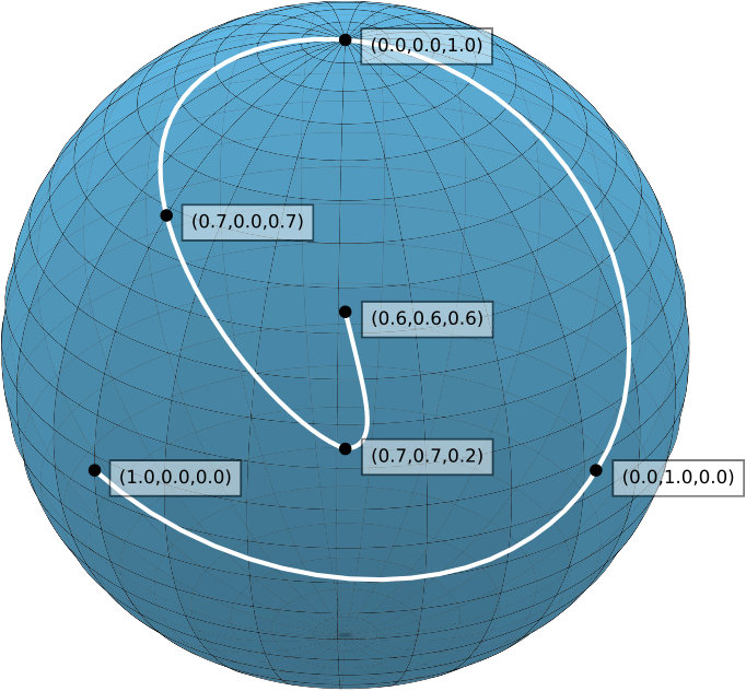 Figure 1
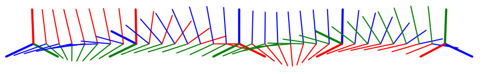 Figure 2
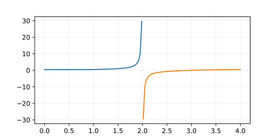 Figure 3
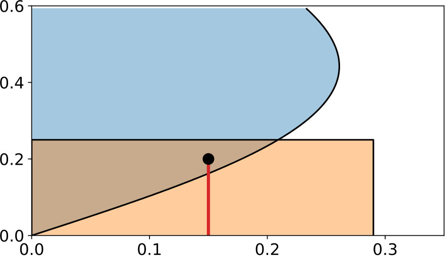 Figure 4
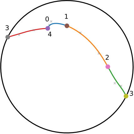 Figure 5
| Implementation | ||||
|---|---|---|---|---|
| Euclidean space | Flat | |||
| -sphere | Sphere | |||
| Hyperbolic space | Hyperbolic | |||
| Real Grassmannian | Grassmannian | |||
| Orthogonal group | ||||
| Complex projective space | Projective | |||
| Complex Grassmannian | ||||
| Unitary group | ||||
| Co-variance matrices |
Peer Reviews
No public reviews on file for this paper yet. If you reviewed it on a platform where reviews are public (OpenReview, ICLR, NeurIPS, ICML), you can paste yours below so the community can read it here.
Videos
No videos yet. Explain this paper in a talk, walkthrough, or lecture? Add one.
A Numerical Algorithm for -splines
on Symmetric Spaces
Klas Modin \[email protected]:[email protected]
Mathematical Sciences, Chalmers and University of Gothenburg, Sweden
Geir Bogfjellmo \[email protected]:[email protected]
Mathematical Sciences, Chalmers and University of Gothenburg, Sweden
Instituto de Ciencias Matemática, Madrid, Spain
Olivier Verdier \[email protected]:[email protected]
Department of Computing, Mathematics and Physics, Western Norway University of Applied Sciences, Bergen, Norway
Abstract
Cubic spline interpolation on Euclidean space is a standard topic in numerical analysis, with countless applications in science and technology. In several emerging fields, for example computer vision and quantum control, there is a growing need for spline interpolation on curved, non-Euclidean space. The generalization of cubic splines to manifolds is not self-evident, with several distinct approaches. One possibility is to mimic the acceleration minimizing property, which leads to Riemannian cubics. This, however, requires the solution of a coupled set of non-linear boundary value problems that cannot be integrated explicitly, even if formulae for geodesics are available. Another possibility is to mimic De Casteljau’s algorithm, which leads to generalized Bézier curves. To construct -splines from such curves is a complicated non-linear problem, until now lacking numerical methods. Here we provide an iterative algorithm for -splines on Riemannian symmetric spaces, and we prove convergence of linear order. In terms of numerical tractability and computational efficiency, the new method surpasses those based on Riemannian cubics. Each iteration is parallel, thus suitable for multi-core implementation. We demonstrate the algorithm for three geometries of interest: the -sphere, complex projective space, and the real Grassmannian.
MSC-2010: 41A15, 65D07, 65D05, 53C35, 53B20, 14M17
Keywords: De Casteljau, cubic spline, Riemannian symmetric space, Bézier curve
Contents
- 1 Introduction
- 2 Generalized Bézier curves on symmetric spaces
- 3 Numerical algorithm
- 4 Examples
- 5 Outlook
- A Identities and bounds on symmetric spaces
- B continuity
- C Convergence of the fixed-point method
- D Python implementation
1 Introduction
We address the following.
Problem 1.1**.**
Given a set of points on a connected manifold , construct a path such that .
For every textbook in numerical analysis teaches cubic splines, i.e., piecewise polynomials of order 3 with matching first and second derivatives. However, the generalization of cubic splines to curved space is non-trivial, essentially because polynomials are not well-defined on manifolds. Interpolating paths on manifolds are, nevertheless, needed in a growing number of applications. In the realization of quantum computers, for example, quantum control of qubits leads to an interpolation problem in complex projective space (see § 4.2). In computer vision, as another example, the recognition of a point cloud up to affine transformations is naturally identified with an element in the Grassmannian (see § 4.3).
If is a Riemannian manifold, a natural generalization of cubic splines are Riemannian cubics [12, 2]. They are based on minimizing acceleration under interpolation constraints, by solving the problem
[TABLE]
The corresponding Euler–Lagrange equation is a fourth order ODE on with complicated, coupled boundary conditions [12]. In addition to the Euclidean case, explicit solutions to the initial-value problem are known for so called null Lie quadratics on and equipped with the bi-invariant Riemannian metric [11]. For other cases, even when geodesics are explicitly known, one is left with numerical ODE methods, combined, for example, with a shooting method to match the boundary conditions. This approach is computationally costly and the associated convergence analysis is involved. Another possibility is to only approximatelly fulfill the interpolation constraints by incorporating them in the minimization functional and then use a steepest-descent method on the space of curves [15]. This approach is also costly.
If is a manifold for which the geodesic boundary problem can be solved explicitly, there is a natural concept of generalized Bézier curves (GBC). They are based on a direct generalization of De Casteljau’s algorithm [13]. Splines can then be constructed by gluing piecewise GBC with matching boundary conditions. In this way, a fully explicit algorithm for -splines on Grassmannian and Stiefel manifolds has been developed [8]. The condition, however, first derived by Popiel and Noakes [14], is significantly more complicated than the condition. For this reason, there is a lack of numerical algorithms for -splines. Nevertheless, continuity is often required in applications, to avoid discontinuities in accelerations.
In this paper we give the first numerical algorithm for -splines based on GBC. Instead of treating all Riemannian manifolds, we focus on the subclass of symmetric spaces (see § 2.1). Such manifolds are of high interest in applications, and include, e.g., spheres, hyperbolic space, real and complex projective spaces, and Grassmannian manifolds (see Table 1). In many cases, the geodesic boundary value problem on a symmetric space has an explicit solution (a prerequisite for De Casteljau’s algorithm). The original condition of Popiel and Noakes is, however, still complicated. We now list the specific contributions of our paper.
Using the special homogeneous space structure of symmetric spaces, we give a significant simplification of the condition (Theorem 2.2). 2. 2.
Using the new condition, we construct an algorithm based on fixed-point iterations (Algorithm 1). 3. 3.
We prove convergence of the algorithm under conditions on the maximal distance between consecutive interpolation points (Theorem 3.1).
The paper is organized as follows. In § 2 we first give a brief description of Riemannian symmetric spaces and thereafter describe the construction of generalized Bézier curves. We also formulate the condition. In § 3 we give the numerical algorithm and we formulate the convergence result. Numerical examples are given in § 4. An outlook towards future work is given in § 5. The proofs of the condition and the convergence result are long and technical, and therefore given in Appendix A-C. In Appendix D we give a brief demonstration of an easy-to-use open-source Python package implementing our interpolation algorithm for several geometries.
2 Generalized Bézier curves on symmetric spaces
Let us describe the construction of generalized Bézier curves on a symmetric space. The construction relies on a notion of interpolation between two points on the manifold, generalizing the notion of a geodesic on a Riemannian manifold [9].
2.1 Symmetric spaces
In this section we briefly recall symmetric spaces. A list of the most common examples of symmetric spaces is given in Table 1. For details, we refer to [16] or [4]. We assume that a Lie group acts transitively on , making a homogeneous space [16, § 4]. We denote the action by
[TABLE]
For every point , we define the isotropy subgroup at
[TABLE]
Now, the homogeneous space is called a symmetric space if the Lie algebra of has a direct sum decomposition
[TABLE]
where is the Lie algebra of , and the summands fulfill the following algebraic conditions
[TABLE]
If these conditions are satisfied at one point , then they are automatically valid at every point with
[TABLE]
where we follow the convention formulated in Appendix A that denotes the canonical action on the space at hand (here, the adjoint action of a Lie group on its Lie algebra).
By differentiating the action map with respect to the arguments, we also obtain, on the one hand, an infinitesimal action of on , and, on the other hand, a prolonged action of on . For and , we denote the infinitesimal action by
[TABLE]
For a fixed , this map induces an isomorphism between and .
2.2 Interpolating Curves
We now define the interpolating curve between two (close enough) points and as the unique curve satisfying
[TABLE]
Let us introduce the notation
[TABLE]
In particular, notice that
[TABLE]
In many (but not all) cases, a symmetric space can be equipped with the structure of a Riemannian manifold, given through an -invariant inner product on . In this case, the interpolating curves are geodesics. From here on, we shall assume that is such a Riemannian symmetric space.
2.3 De Casteljau’s construction
We briefly describe the De Casteljau construction, illustrated on Figure 1. This algorithm constructs Bézier curves from interpolating curves. We focus on cubic Bézier curves. From four points , , and , one defines the cubic Bézier curve by
[TABLE]
Note that, by construction, and .
2.4 Exponential and logarithm on symmetric spaces
For the condition in § 2.5 and implementation of the algorithm we need the following functions (see Figure 2).
The action of a group element on a point :
[TABLE] 2. 2.
A movement function , which, to a point and a velocity at , assigns an element . This function should generate interpolating curves (6), i.e., it should be of the form
[TABLE] 3. 3.
The logarithm; given two points and in , it is defined by
[TABLE]
Throughout the paper we make the blanket assumption that and are never past conjugate points, so that the logarithm is always well-defined.
2.5 Cubic splines and condition
We shall now consider curves consisting of piecewise cubic Bézier curves. As we have seen in § 2.3, each cubic Bézier curve is determined by two interpolating points and two control points. To construct a curve of piecewise Bézier curves we therefore need to impose conditions on the control points (in addition to the interpolating conditions). On Euclidean space, the standard approach is to use the conditions for continuity at the interpolating points, which leads to a linear set of equations. On a general Riemannian manifold, the corresponding condition, given by Popiel and Noakes [14], is highly nonlinear, involving the inverse of the derivative of the Riemannian exponential. In the special case of symmetric spaces, however, we now show that the condition simplifies significantly, involving only the three operations (9), (10), and (11).
Definition 2.1**.**
Let be points on a symmetric space . A composite cubic Bézier curve on is a curve such that for each integer , , and such that for each integer , the restriction is a cubic Bézier curve (as defined in § 2.3). To each such piece , we associate two control points, denoted and . A -continuous composite cubic Bézier curve is called a cubic spline.
The interpolating conditions ensure that is continuous (or ). However, for higher degree of continuity ( or ), we need additional conditions on the control points. We now give such conditions.
Theorem 2.2**.**
Let be a Riemannian symmetric space and let be a composite cubic Bézier curve according to § 2.5. Consider the conditions on the control points given by
[TABLE]
- (i)
If condition (12) is fulfilled, then is a -curve. 2. (ii)
If conditions (12) and (13) are fulfilled, then is a -curve, i.e., a cubic spline.
Furthermore, if fulfills the conditions (12) and (13), then it is uniquely determined either by clamped boundary conditions, where and are prescribed, or by natural boundary conditions, where .
Remark 2.3**.**
Notice how (12) and (13) are generalizations of the first and second order finite differences in Euclidean geometry. Indeed, in this case condition (12) reads
[TABLE]
and condition (13) reads
[TABLE]
See Figure 3 for a geometric illustration of the condition (13).
Outline of proof.
The details of the proof are rather technical and therefore given in Appendix B. However, for convenience we also provide an outline here:
- (i)
The condition in the case of Riemannian symmetric spaces is given by Popiel and Noakes [14, Sec. 4], expressed in terms of the derivative of the symmetry function . 2. (ii)
Using the special symmetric space structure, we show that the derivative of can be expressed solely in terms of the movement function (Appendix A). 3. (iii)
Together with a result on equivariance of the function (Appendix A) we can then simplify the original Riemannian symmetric space condition by Popiel and Noakes [14] to the one given by (13).
∎
3 Numerical algorithm
We shall now construct a fixed point iteration algorithm for cubic splines on symmetric spaces, based on the condition in Theorem 2.2. To this end, we parameterize the control points and by the corresponding tangent vectors as defined in Theorem 2.2. Next, let
[TABLE]
The iteration map over is then given by
[TABLE]
where
[TABLE]
Pseudo code for the complete algorithm is given in Algorithm 1. We consider two options for boundary conditions.
- (i)
Clamped spline:
[TABLE]
where and are prescribed constants. 2. (ii)
Natural spline:
[TABLE]
3.1 Convergence result
In this section we give a result on convergence of the fixed point method given by Algorithm 1. To do so, we first give some preliminary definition.
The Riemannian distance between is denoted by . Our proof of convergence uses that two consecutive points are close. Thus, we define the constant
[TABLE]
The other constant that comes into play is a bound on (essentially) the curvature of . Indeed, if denotes the -invariant norm on associated with the Riemannian structure of , then we define the constant as
[TABLE]
If is flat, then . If is the -sphere of radius , then .
Our convergence result is now formulated as follows.
Theorem 3.1**.**
If is sufficiently small, then Algorithm 1 with natural boundary conditions converges linearly. If and are both sufficiently small, then Algorithm 1 with clamped boundary conditions converges linearly.
Outline of proof.
Again, the proof is long and technical, and therefore given in Appendix C. Here we give a brief outline.
The proof is based on showing that the iteration mapping (17) is a contraction. For convenience, we use the variables instead of . The iteration mapping is denoted .
- (i)
The first step is to give an invariant region of the iteration mapping. This is given in § C.1, which proves existence of (depending on both and ), such that implies . 2. (ii)
The next step is to prove that is a contraction, which is established by a series of estimates on the partial derivatives on (§ C.2, § C.2, and § C.2). These estimates depend on . 3. (iii)
The final step, in § C.3, is to use the contraction mapping theorem.
∎
4 Examples
4.1 Unit quaternions
Unit quaternions (versors) are used extensively in computer graphics to represent 3-D rotations. They are elements of the form with
[TABLE]
Thus, we can identify unit quaternions with . In turn, is a double cover of . A point on therefore gives a rotation matrix, and likewise any rotation matrix corresponds to two antipodal points on . The rotation of a vector by a unit quaternion can be compactly written using quaternion multiplication as
[TABLE]
where is thought of as a pure imaginary quaternion.
Since is a Riemannian symmetric space (with respect to the standard Riemannian metric), we can use Algorithm 1 to obtain continuous spline interpolation between rotations. Since geodesics on are given by great circles, it is straightforward to derive the mappings and .
The resulting -curve interpolating 5 orientations is shown in Figure 5. In the figure, an element is represented by the rotated basis vectors
[TABLE]
The actual interpolation points are marked with bolder lines.
Note that can be canonically identified with . Note also that has a symmetric space structure as the quotient [10]. Here, however, we considered the symmetric space structure . These two symmetric space structure are locally equivalent. This is because, is a double cover of and is a double cover of . Our algorithm gives the same result regardless of the choice of either of those two symmetric space structures on . From this point of view, our algorithm could be used for spline interpolation on any compact Lie group , using the Cartan–Schouten symmetric space structure .
4.2 Quantum states
The control of quantum states is an important subproblem in quantum information and the realization of quantum computers [3]. The objective is to find a time-dependent Hamiltonian designed to ‘steer’ a given quantum state through a sequence of states at given times . As instantaneous switching of the Hamiltonian is not experimentally feasible [1], the interpolating curve should be at least continuous.
If the quantum state space is finite dimensional, corresponding to an ensemble of qubits, then, in the geometric description of quantum mechanics [6, 7], the phase space is given by complex projective space . The quantum control problem can then be seen as a two-step process:
Find an interpolating curve such that and . 2. 2.
Using the homogeneous structure , lift to a curve such that and .111The lifting is, of course, not unique. It is natural to minimize the change in Hamiltonian , as suggested by Brody, Holm, and Meier [1]. The time-dependent Hamiltonian is then given by .
We can use Algorithm 1 for the first step. (The second step is not treated in this paper.)
The simplest case of a single qubit corresponds to the phase space , which is isomorphic to a sphere (called the Bloch sphere). Using 6 interpolation points, the resulting interpolating curve is visualized on the Bloch sphere in Figure 6.
4.3 Affine shapes
The space of affine shapes is the quotient set whose elements consist of labelled (i.e. ordered) points in defined up to affine transformations. Thus, and define the same affine shape if there exists an affine transformation such that . The study of affine shapes has many applications in computer vision [5]. An example is the identification of planar surfaces (such as facades of buildings) in images taken from different projection angles.
The space of affine shapes with full rank (meaning that the points are not contained in an affine hyperplane of ) can be identified with the real Grassmannian manifold of -dimensional subspaces in . Indeed, choose a coordinate system and place the coordinates of the vectors column by column in an matrix. The kernel of this matrix is then a subspace of . The full rank assuption means that the kernel has dimension . This gives us a point in , which, by the canonical isomorphism between and , gives a point in .
Since the Grassmannian is a symmetric space, we can use our algorithm to construct -splines between affine shapes.
Let us study a particular case of affine shapes corresponding to points in . Our aim is to create a spline between such shapes, defined by (A)–(D) in Figure 7. For every shape, we obtain a matrix of full rank, which defines our element in . We then use Algorithm 1 to construct a spline interpolating the points in .
To visualize the result, notice that is isomorphic to the real projective plane . Indeed, this follows since the kernels of the matrices are one dimensional, that is, they are directions in . We may therefore visualise the affine shapes as follows. First, we compute the intersection of the kernel direction with the half-sphere
[TABLE]
We then compute the stereographic projection from the point of coordinate . This function is explicitly given by
[TABLE]
The resulting projected spline curve is plotted in Figure 8.
We stress that interpolation of affine shapes cannot, in general, be accomplished by standard spline interpolation in vector spaces. Indeed, if we introduce local coordinates by expressing the point in the basis spanned by the basis vectors and with origin at , then the -coordinate is infinite as the spline passes through the affine shape (C). This is illustrated in Figure 9. More generally, any local coordinate chart would have similar artifacts for some shapes.
5 Outlook
There are a number of possible extensions of our methods and proofs to be studied in future work. Here we list some of them.
- •
We surmise that the conditions of Theorem 2.2 are in fact valid for more general symmetric spaces than Riemannian ones. In particular, we would like to be able to prove that result directly, without resorting to the previous result of Popiel and Noakes, which is the only reason for us to restrict to the Riemannian symmetric space case at this point.
- •
The only structure that we need to implement Algorithm 1 and to state Theorem 2.2 is an invariant connection (see (26a)), which only requires the homogeneous space at hand to be reductive [10, § 4]. We would expect similar results in that case, which would for instance cover arbitrary Lie groups, as well as Stiefel manifolds.
- •
A modification of our algorithm is possible in the more general case of arbitrary Riemannian manifolds (not necessarily symmetric), using the original condition of Popiel and Noakes [14]. We are working on an implementation and a proof of convergence.
- •
Our algorithm is currently based on a fixed point iteration. One could instead use a Newton iteration, which would ensure convergence in one step in the Euclidean case.
Acknowledgments
This project has received funding from the European Union’s Horizon 2020 research and innovation programme under grant agreement No 661482, from the Swedish Foundation for Strategic Research under grant agreement ICA12-0052, and from the Knut and Alice Wallenberg Foundation under grant agreement KAW-2014.0354.
Appendix A Identities and bounds on symmetric spaces
In this section we prove several identities and bounds on (Riemannian) symmetric spaces which are used in Appendix B and Appendix C below.
Let be a symmetric space, where and is the decomposition described in § 2.1, and let be the canonical projection. Denote by and the maps
[TABLE]
as usual, and are defined by
[TABLE]
and we identify to define
[TABLE]
By an abuse of notation, we will use to denote any of the following action maps
[TABLE]
The notation is used to denote the natural pairing of one-forms and tangent vectors over a point .
The infinitesimal action (5) and the decomposition define a principal connection [10], i.e., a -valued one-form on which fulfills
[TABLE]
for all .
By construction, .
Throughout this section and the following, denotes the trivialized derivative of the Lie group exponential, that is
[TABLE]
where the last equality follows from differentiating .
Lemma A.1**.**
Fix , and define by . Then
[TABLE]
Proof.
By the properties of a Lie group action, for , we have
[TABLE]
We differentiate by the product rule and get
[TABLE]
where the final equality is because for all . ∎
Lemma A.2**.**
Fix . Let , then
[TABLE]
Proof.
As a function , is an analytic function of with Taylor series . Using the definition (4) of a symmetric space, we have, for any element , that
[TABLE]
The effect of is thus to eliminate terms in , leaving only the terms with an even exponent , so
[TABLE]
Note that, as is an even function of , we have
[TABLE]
∎
A corollary of Appendix A is that for near zero, is invertible as a function with inverse given by .
Lemma A.3**.**
Fix . Let be the symmetry function at , i.e., and let , . Then
[TABLE]
Proof.
Let . Then is a local diffeomorphism and . Differentiating both and with respect to , and using Appendix A, we get
[TABLE]
Since is a diffeomorphism, we can choose such that , i.e., . Using Appendix A, we also have , and the result follows. ∎
Lemma A.4**.**
Let , and . Then
[TABLE]
Proof.
Let be the interpolating curve between and . Then , and differentiating at , we get
[TABLE]
∎
For the final lemmata, we assume to be a Riemannian symmetric space. This is equivalent to the existence of an -invariant inner product on , from which we derive a norm on .
Lemma A.5**.**
Let , then
[TABLE]
(Notice , not , in the last denominator.)
Proof.
We use Appendix A to set . The lemma at hand then follows from considering the infinite series for and its inverse, as well as the definition of the curvature in equation (22). ∎
Lemma A.6**.**
Fix . Let , and . Recall from § 3.1 that is the Riemannian distance between two points on . Let us define
[TABLE]
We then have the inequality
[TABLE]
Proof.
Let be the geodesic from to , and let be such that
[TABLE]
Then , . We note that, by the triangle inequality, we have
[TABLE]
Differentiating (27) we get
[TABLE]
which we rewrite as
[TABLE]
where we have used that for all . Taking norms on both sides and using that acts by isometries, we have
[TABLE]
Moreover, by Appendix A,
[TABLE]
We now use the monotonicity of , and the bound (28) to obtain
[TABLE]
∎
Appendix B continuity
We now prove Theorem 2.2. The proof relies on a result by Popiel and Noakes [14].
Proof of Theorem 2.2.
At non-integer , the spline is . We show that the spline is at , i.e., at the interpolating points . By [14, Thm. 3], a sufficient and necessary condition for the spline to be at is
[TABLE]
where is the symmetry function at . We proceed by removing the dependence of in (29) by using the lemmata from Appendix A.
Recall that and . By Appendix A, we have
[TABLE]
Using Appendix A, with , we can write
[TABLE]
Next, we note that
[TABLE]
Using (30) and (31), we can rewrite (29) as
[TABLE]
Acting on the whole equation from the left with and rearranging, we get
[TABLE]
We now obtain the condition (13) by using the condition (12) to replace in the equation above. ∎
Appendix C Convergence of the fixed-point method
We now proceed to prove Theorem 3.1, i.e., that if consecutive interpolation points are sufficiently close then Algorithm 1 converges to a solution. In the proof, we will work with variables in the Lie algebra . Let
[TABLE]
and let
[TABLE]
be the Lie algebra elements defined by
Switching to variables in the Lie algebra, the fixed-point iteration (17) becomes a map
[TABLE]
For , . To simplify notation, we define by
[TABLE]
Now, for the fixed-point iteration map can be expressed as
[TABLE]
and both and are given by the boundary conditions
[TABLE]
Specifically, for clamped boundary conditions, we get
[TABLE]
where and are prescribed. For free boundary conditions
[TABLE]
It is convenient to introduce the auxiliary variables
[TABLE]
and to write where
[TABLE]
Furthermore, we define the norms
[TABLE]
and
[TABLE]
Recall that denotes the maximum distance between neighbouring interpolation points as declared in equation (21). Notice that by the triangle inequality, we have
[TABLE]
and similarly for , so
[TABLE]
We are now in position to prove Theorem 3.1. The proof consists in showing the existence of an invariant region, and thereafter bounding the partial derivatives of to show that it is a contraction.
C.1 Invariant region
We begin by establishing an invariant region.
Proposition C.1**.**
Let satisfy the inequality
[TABLE]
where . If either one of the following boundary conditions is fulfilled:
- (i)
clamped spline boundary conditions are used, , and , 2. (ii)
natural spline boundary conditions are used and ,
then we also have .
To reach this result, we first prove a few bounds for .
Lemma C.2**.**
Let , then the following bounds hold,
[TABLE]
where .
Proof.
We prove the first inequality. The proof of the second inequality is entirely symmetrical and therefore omitted.
By definition (35),
[TABLE]
The proof uses Appendix A to bound .
Recall that acts isometrically on by the adjoint action
[TABLE]
where and are vectors in . We also have
[TABLE]
and
[TABLE]
By Appendix A, we have
[TABLE]
where
[TABLE]
From the triangle inequality, we have
[TABLE]
Thus , and the claim follows by monotonicity of the function . ∎
Proof of § C.1.
Using § C.1, and the inequalities and , we get that
[TABLE]
for all .
For the boundary velocities:
- (i)
Clamped spline: , so by our assumption. 2. (ii)
Natural spline: , so
[TABLE]
under a weaker condition on . Similarly for .
In conclusion, under the assumption (38), we have
[TABLE]
and \big{\{}\,\bm{\xi}\;\big{|}\;\lVert\bm{\xi}\rVert\leq V\,\big{\}} forms an invariant region. ∎
C.2 Contraction
We now establish that, for and sufficiently small, there exists an such that, in the operator norm derived from (36) . We first consider the effect of varying and in .
Proposition C.3**.**
Let and denote by the partial derivative of with respect to , i.e. is a linear operator . Then, in the operator norm,
[TABLE]
and
[TABLE]
Proof.
We only prove the first claim. The proof of the second is entirely symmetrical. The term only enters through the term , so
[TABLE]
By the definition of , we have
[TABLE]
Differentiating implicitly on both sides, then acting from the left by , we get
[TABLE]
where . Taking norms on both sides, and using that the group action is isometric, we get
[TABLE]
and
[TABLE]
It follows that
[TABLE]
thus
[TABLE]
The claims in the proposition follow from (39) and Appendix A. ∎
We note that we can also use a Taylor expansion of the right hand side to get the asymptotic bound
[TABLE]
To bound , it is again advantageous to do the splitting , and consider each term separately.
While it is possible to bound by trigonometric and hyperbolic functions of and , the required calculations are lengthy, and we restrict ourself to an asymptotic bound.
Proposition C.4**.**
Let and denote by the partial derivative of with respect to . In the operator norm
[TABLE]
and
[TABLE]
Again, we will only prove the first claim, the proof of the second is entirely symmetrical. We first prove the following Lemma on the derivative of .
Lemma C.5**.**
For , the following equality holds
[TABLE]
Proof.
We use that
[TABLE]
By differentiating implicitly, we get
[TABLE]
where the second equality uses (40). Acting from the left with , we get
[TABLE]
Applying the connection to both sides, we get
[TABLE]
where the bracketed expressions are linear operators . Now, the map is invertible by Appendix A, and the claim follows. ∎
We now proceed with the proof of § C.2.
Proof of § C.2.
From the definition of ,
[TABLE]
Using § C.2, we have
[TABLE]
Using Appendix A, the series expansions for , and , the expression on the right hand side can be expanded as an infinite series in and applied to . (Recall that, as we saw in the proof of Appendix A, the effect of is to cancel out Lie monomials of even degree.) The crucial point is that there is a cancellation in the leading term so that, neglecting terms of fourth order and higher,
[TABLE]
We thus get
[TABLE]
The proposition follows by taking norms. ∎
It is also possible to bound the derivatives of the boundary condition functions.
Proposition C.6**.**
**
- (i)
(Clamped splines) Let and be as in (32). Then , . 2. (ii)
(Natural splines) Let and be as on (33). Then
[TABLE]
and similar for .
Proof.
- (i)
For clamped splines, and are constant. 2. (ii)
For natural splines, we have
[TABLE]
Differentiating and taking norms, we get
[TABLE]
where . Appendix A now gives
[TABLE]
and the claim follows by a Taylor expansion of and . The corresponding bound and proof for is entirely symmetrical.
∎
C.3 Convergence
We are now ready to prove the convergence theorem.
Proof of Theorem 3.1.
A consequence of § C.1 is that has an invariant region for small enough . We need to also establish that it is a contraction. It is sufficient to show that there exists an such that in an invariant region.
We have
[TABLE]
as well as
[TABLE]
By § C.2, § C.2, and § C.2, we can bound the terms appearing with a Taylor expansion to obtain
[TABLE]
We can now use (37) and § C.2 to obtain a bound of the form
[TABLE]
It is therefore clear that when is sufficiently small, is a contraction. When approaches zero, the smallest satisfying (38) also approaches zero. Therefore, when is small enough, there is a such that
- •
\Big{\{}\,\bm{\xi}\;\Big{|}\;\lVert\bm{\xi}\rVert\leq V\,\Big{\}} is a compact invariant region and
- •
is a contraction on that region.
Therefore, the fixed point iteration converges to a solution. ∎
See Figure 10 for an illustration of the final argument in the proof.
Appendix D Python implementation
Here we briefly indicate how to use our Python implementation to compute splines in various geometries. First, one has to install the following package by following the installation instructions:
https://github.com/olivierverdier/bsplinelab
The minimal necessary import is
Here is an example of how to interpolate between random points in the Euclidean case:
interpolation_points = np.random.rand(10,4)
b = cubic_spline(Symmetric, interpolation_points)
The result is then a function b which is equal to the interpolation points at integer points on the interval .
In order to interpolate on, for instance, a sphere, one would do as follows:
3 points on the sphere:
interpolation_points = np.array([[1.,0,0], [0,1,0], [0,0,1]])
b = cubic_spline(Symmetric, interpolation_points, geometry=Sphere())
The function b is now a function defined on the interval such that it is , is interpolating the prescribed points at the integer points [math], and , and is on the sphere for all points in between.
For further information on bsplinelab, we refer to the package documentation and the available code examples.
The reference list from the paper itself. Each links out to its DOI / PubMed record.
- 1Brody et al. [2012] D. C. Brody, D. D. Holm, and D. M. Meier, Quantum splines, Phys. Rev. Lett. 109 (2012), 100501.
- 2Crouch and Leite [1991] P. Crouch and F. S. Leite, Geometry and the dynamic interpolation problem, American Control Conference, 1991 , pp. 1131–1136, IEEE, 1991.
- 3Dong and Petersen [2010] D. Dong and I. R. Petersen, Quantum control theory and applications: a survey, IET Control Theory & Applications 4 (2010), 2651–2671.
- 4Helgason [1962] S. Helgason, Differential Geometry and Symmetric Spaces , American Mathematical Society, 1962.
- 5Kendall et al. [2009] D. Kendall, D. Barden, T. Carne, and H. Le, Shape and Shape Theory , Wiley, 2009.
- 6Kibble [1978] T. W. B. Kibble, Relativistic models of nonlinear quantum mechanics, Comm. Math. Phys. 64 (1978), 73–82.
- 7Kibble [1979] T. W. B. Kibble, Geometrization of quantum mechanics, Comm. Math. Phys. 65 (1979), 189–201.
- 8Krakowski et al. [2017] K. A. Krakowski, L. Machado, F. Silva Leite, and J. Batista, A modified Casteljau algorithm to solve interpolation problems on Stiefel manifolds, J. Comput. Appl. Math. 311 (2017), 84–99.