A regularization approach for an inverse source problem in elliptic systems from single Cauchy data
Michael Hinze, Bernd Hofmann, Tran Nhan Tam Quyen

TL;DR
This paper develops a Tikhonov-type regularization method for identifying sources in elliptic systems from single boundary measurements, providing convergence analysis, error bounds, and a numerical solution approach.
Contribution
It introduces a novel regularization approach for inverse elliptic problems with theoretical convergence and error analysis, supported by numerical experiments.
Findings
Convergence of finite element approximations to the inverse problem solutions.
Derivation of error bounds and convergence rates under source conditions.
Numerical validation using a conjugate gradient method.
Abstract
In this paper we investigate the problem of identifying the source term in an elliptic system from a single noisy measurement couple of the Neumann and Dirichlet data. A variational method of Tikhonov-type regularization with specific misfit term of Kohn-Vogelius-type and quadratic stabilizing penalty term is suggested to tackle this linear inverse problem. The method also appears as a variant of the Lavrentiev regularization. For the occurring linear inverse problem in infinite dimensional Hilbert spaces, convergence and rate results can be found from the general theory of classical Tikhonov and Lavrentiev regularization. Using the variational discretization concept, where the PDE is discretized with piecewise linear and continuous finite elements, we show the convergence of finite element approximations to solutions of the identification problem. Moreover, we derive an error bound and…
Click any figure to enlarge with its caption.
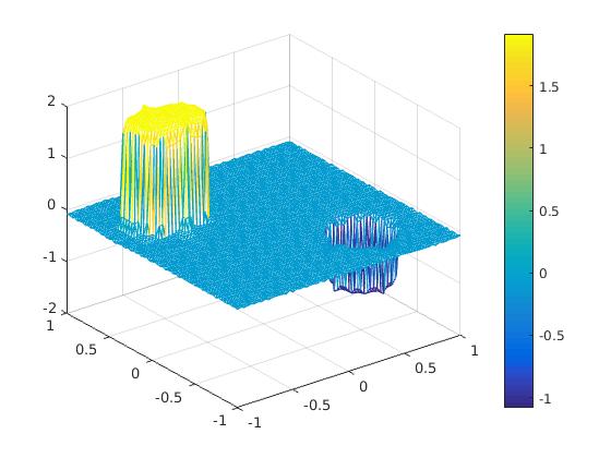 Figure 1
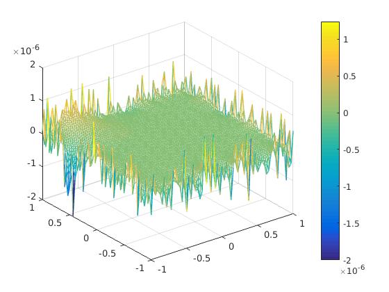 Figure 2
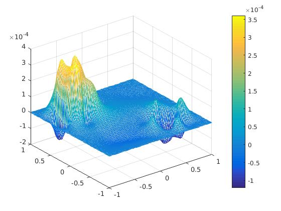 Figure 3
 Figure 4
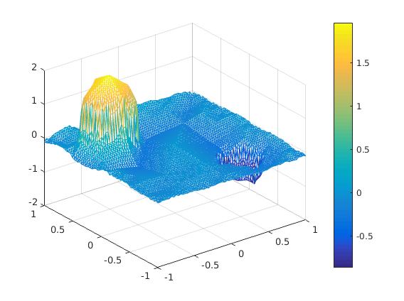 Figure 5
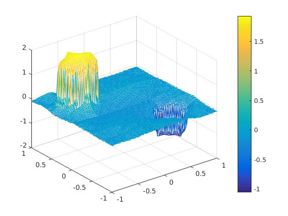 Figure 6
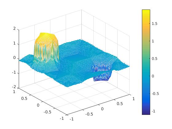 Figure 7
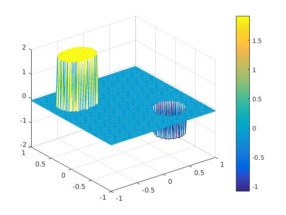 Figure 8
| Convergence history | |||||
|---|---|---|---|---|---|
| Iterate | Tolerance | ||||
| 4 | 0.7071 | 0.7071e-2 | 0.1916 | 312 | -3.0822e-5 |
| 8 | 0.3536 | 0.3536e-2 | 9.3172e-2 | 387 | -1.2739e-6 |
| 16 | 0.1766 | 0.1766e-2 | 4.1174e-2 | 461 | -1.4029e-6 |
| 32 | 8.8388e-2 | 0.8839e-3 | 2.0932e-2 | 505 | -1.8559e-7 |
| 64 | 4.4194e-2 | 0.4419e-3 | 7.2765e-3 | 579 | -7.3540e-9 |
| Convergence history | |||||
|---|---|---|---|---|---|
| 4 | 0.5215 | 2.0441e-2 | 2.0396e-2 | 6.9952e-2 | 6.9713e-2 |
| 8 | 0.3309 | 6.3175e-3 | 6.3083e-3 | 3.1374e-2 | 3.1311e-2 |
| 16 | 0.1915 | 2.0132e-3 | 2.0122e-3 | 1.7276e-2 | 1.7243e-2 |
| 32 | 0.1073 | 5.5434e-4 | 5.5426e-4 | 8.9136e-3 | 8.9130e-3 |
| 64 | 5.2568e-2 | 1.4669e-4 | 1.4666e-4 | 3.9352e-3 | 3.9347e-3 |
| Experimental order of convergence | |||||
|---|---|---|---|---|---|
| EOC | EOC | EOC | EOC | EOC | |
| 4 | – | – | – | – | – |
| 8 | 0.6563 | 1.6940 | 1.6930 | 1.1568 | 1.1548 |
| 16 | 0.7891 | 1.6499 | 1.6485 | 0.8608 | 0.8607 |
| 32 | 0.8357 | 1.8606 | 1.8601 | 0.9547 | 0.9520 |
| 64 | 1.0294 | 1.9180 | 1.9181 | 1.1796 | 1.1797 |
| Mean of EOC | 0.8276 | 1.7806 | 1.7799 | 1.0380 | 1.0368 |
| Numerical results for , with multiple observations | ||||||||
|---|---|---|---|---|---|---|---|---|
| Iterate | Tolerance | |||||||
| 1 | 531 | -3.2313e-8 | 0.3292 | 0.3280 | 5.9096e-3 | 5.9090e-3 | 0.1225 | 0.1221 |
| 6 | 517 | -7.1620e-9 | 0.3331 | 0.2583 | 4.3125e-3 | 4.3122e-3 | 7.9322e-2 | 7.9320e-2 |
| 16 | 536 | -6.4706e-8 | 0.3289 | 0.1747 | 2.8465e-3 | 2.8461e-3 | 5.2318e-2 | 5.2314e-2 |
Peer Reviews
No public reviews on file for this paper yet. If you reviewed it on a platform where reviews are public (OpenReview, ICLR, NeurIPS, ICML), you can paste yours below so the community can read it here.
Videos
No videos yet. Explain this paper in a talk, walkthrough, or lecture? Add one.
Taxonomy
TopicsNumerical methods in inverse problems · Advanced Mathematical Modeling in Engineering · Composite Material Mechanics
A regularization approach for an inverse source problem in elliptic systems from single Cauchy data
Michael Hinzea††Email: [email protected], [email protected], [email protected], Bernd Hofmannb and Tran Nhan Tam Quyenc
aDepartment of Mathematics, University of Hamburg, 20146 Hamburg, Germany
bFaculty of Mathematics, Chemnitz University of Technology, 09107 Chemnitz, Germany
cInstitute for Numerical and Applied Mathematics, University of Goettingen, 37083 Goettingen, Germany
Abstract: In this paper we investigate the problem of identifying the source term in the elliptic system
[TABLE]
from a single noisy measurement couple of the Neumann and Dirichlet data with noise level . In this context, the diffusion matrix is given. A variational method of Tikhonov-type regularization with specific misfit term of Kohn-Vogelius-type and quadratic stabilizing penalty term is suggested to tackle this linear inverse problem. The method also appears as a variant of the Lavrentiev regularization. For the occurring linear inverse problem in infinite dimensional Hilbert spaces, convergence and rate results can be found from the general theory of classical Tikhonov and Lavrentiev regularization. Using the variational discretization concept, where the PDE is discretized with piecewise linear and continuous finite elements, we show the convergence of finite element approximations to solutions of the regularized problem. Moreover, we derive an error bound and corresponding convergence rates provided a suitable range-type source condition is satisfied. For the numerical solution we propose a conjugate gradient method. To illustrate the theoretical results, a numerical case study is presented which supports our analytical findings.
Key words and phrases: Inverse source problem, Tikhonov and Lavrentiev regularization, finite element method, source condition, convergence rates, ill-posedness, conjugate gradient method, Neumann problem, Dirichlet problem.
AMS Subject Classifications: 35R25; 47A52; 35R30; 65J20; 65J22.
1 Introduction
Let be an open, bounded and connected domain of with Lipschitz boundary . We consider the elliptic system
[TABLE]
where is the unit outward normal on and the diffusion matrix is given. Furthermore, we assume that is symmetric and satisfies the uniformly ellipticity condition
[TABLE]
for all with some constant .
The system (1.1)–(1.3) is overdetermined, i.e. if the Neumann and Dirichlet boundary conditions , and the source term are given, then there may be no satisfying this system. In this paper we assume that the system is consistent and our aim is to reconstruct a function in the system (1.1)–(1.3) from a noisy measurement couple of the exact Neumann and Dirichlet data \big{(}j^{\dagger},g^{\dagger}\big{)}, where stands for the measurement error, i.e. we assume the noise model
[TABLE]
The source identification problem in PDEs arises in many branches of applied science such as electroencephalography, geophysical prospecting and pollutant detection, and attracted great attention from many scientists in the last 30 years or so. For surveys on this subject we may consult in [7, 15, 18, 22, 25, 42] and the references therein. Up to now, only a limited number of works was investigated the general source identification problem and obtained results concentrated on numerical analysis for the identification problem. In [19, 31, 32] authors have used the dual reciprocity boundary element methods to simulate numerically for the above mentioned identification problem. In case some priori knowledge of the identified source is available, such as a point source, a characteristic function or a harmonic function, numerical methods treating the problem have been obtained in [5, 6, 30, 39]. A survey of the problem of simultaneously identifying the source term and coefficients in elliptic systems from distributed observations can be found in [38], where further references can be found.
In the present paper, the general source identification problem in elliptic partial differential equations from a single noisy measurement couple of Neumann and Dirichlet data is studied. So far, we have not yet found investigations on the discretization analysis for this source recovery problem, a fact which also motivated the research presented in the paper. By using a suitable version of the Tikhonov-type regularization with some non-standard misfit term we could outline that the source distribution inside the physical domain can be reconstructed from a finite number of observations on the boundary , at least by numerical approximations. The specific regularization approach proves to be a version of Lavrentiev regularization with implicit forward operator. One of the main results of the paper is to show convergence of the finite element discretized Tikhonov-regularized solutions to a sought source function. Another main result is the interpretation of an occurring condition of solution smoothness as a range-type source condition of Lavrentiev’s regularization method. This allows us to establish error bounds and corresponding convergence rates for the regularized solutions.
To formulate precisely the problem, we first give some notations. Let us denote by the continuous Dirichlet trace operator with its continuous right inverse operator, i.e. for all . We set
[TABLE]
and denote by the positive constant appearing in the Poincaré-Friedrichs inequality (cf. [35])
[TABLE]
Since , the inequality (1.6) is in particular valid for all . Furthermore, by (1.4), the coercivity condition
[TABLE]
holds for all .
Now, for any fixed we can simultaneously consider the Neumann problem
[TABLE]
as well as the Dirichlet problem
[TABLE]
By the aid of (1.7) and the Riesz representation theorem, we conclude that for each there exists a unique weak solution of the problem (1.8) in the sense that and satisfies the identity
[TABLE]
for all , where notation stands for the value of the function at and the notation is the inner product of and in the space . Then we can define the Neumann operator
[TABLE]
which maps each to the unique weak solution of the problem (1.8). Similarly, the problem (1.9) also attains a unique weak solution in the sense that , and the identity
[TABLE]
holds for all . The Dirichlet operator is defined as
[TABLE]
which maps each to the unique weak solution of the problem (1.9). Therefore, for any fixed we can define the so-called Neumann-to-Dirichlet map
[TABLE]
We mention that since , we from (1.10) have that for all . In view of (1.11) we therefore conclude , where the identities
[TABLE]
are satisfied, and the operators and are linear and bounded from into itself. Furthermore, , where is linear, self-adjoint, bounded and invertible, as the diffusion is smooth enough (cf. [33]).
As in electrical impedance tomography (EIT) or for the Calderón’s problem [4, 14, 33] one can pose the question whether the source distribution inside a physical domain can be determined from an infinite number of observations on the boundary , i.e. from the Neumann-to-Dirichlet map :
[TABLE]
To the best of our knowledge, the above question is still open so far. In case an observation of being available one can use a certain regularization method to approximate the sought source. For example, one can consider for operator norms a minimizer of the problem
[TABLE]
as a reconstruction along the lines of Tikhonov’s regularization method, where is the regularization parameter and is an a-priori estimate of the sought source.
However, in practice we have only a finite number of observations and the task is to reconstruct the identified source, at least by numerical approximations. Furthermore, for simplicity of exposition we below restrict ourselves to the case of just one observation pair being available, while the approach described here can be easily extended to multiple measurements , see Section 6, Ex. 6.2. The inverse problem is thus stated as follows.
[TABLE]
In other words, the interested problem is, for given , to find some and consequently such that the system (1.1)–(1.3) is satisfied in the weak sense. Precisely, we define the general solution set
[TABLE]
of the inverse problem . The source identification problem as described here is well known to be not uniquely determined from boundary observations (see a counterexample in [3]), i.e. the set fails to be a singleton. Since not the Neumann-to-Dirichlet map is given, but only one pair , the problem is even highly underdetermined. Thus instead we will search for the uniquely determined -minimum-norm solution , which is the minimizer of the problem
[TABLE]
As a consequence of item (iii) of Lemma 2.1 below, the set is non-empty, closed and convex, hence is uniquely determined. On the other hand, for all the equation is fulfilled. However, we have to solve this equation with noise data of satisfying (1.5). The simplest variety of regularization may be to consider a minimizer of the Tikhonov functional
[TABLE]
over as an approximation solution to .
In present work we adopt the variational approach of Kohn and Vogelius [27, 28, 29] in using cost functional containing the gradient of forward operators to the above mentioned inverse source problem. More precisely, we use the convex functional
[TABLE]
instead of the mapping , together with Tikhonov regularization and consider the unique solution of the strictly convex minimization problem
[TABLE]
where the gradient of the functional can be explicitly written as
[TABLE]
The motivation in using this cost functional as misfit functional is that for all the inequality
[TABLE]
holds true and at any . The advantage is evident, because the minimizer satisfies the equation such that, for , and , we have
[TABLE]
and hence, for , we have
[TABLE]
Due to formula (1.18), the Tikhonov regularization approach under consideration with specific misfit term also appears as a variant of the Lavrentiev regularization (see, e.g., [2, 12, 24, 43]). After some operator-theoretic settings and preliminary results in Section 2, concerning also the ill-posedness of the linear inverse problem under consideration, we apply in Section 3 the general theory of classical Tikhonov and Lavrentiev regularization for such problems yielding propositions on convergence and convergence rates for the regularized solutions in the infinite dimensional Hilbert spaces. However, for convenience in numerical analysis with the finite element methods introduced in Section 4 our focus is here on the extremal problem for minimizing the Tikhonov functional with Kohn-Vogelius misfit term and quadratic penalty. The use of different convex penalty terms, e.g. total variation, may be a work for us in future.
Let and be corresponding approximations of the solution maps and in the finite dimensional space of piecewise linear, continuous finite elements. We then consider the discrete regularized problem corresponding to , i.e., the following strictly convex minimization problem
[TABLE]
Using the variational discretization concept introduced in [23], we show in Section 4 that the unique solution of the problem automatically belongs to the finite dimensional space . Thus, a discretization of the admissible set can be avoided.
As and with an appropriate a-priori regularization parameter choice , also in Section 4, we prove that the sequence \big{(}f^{h}_{\rho,\delta}\big{)} converges to in the -norm. Furthermore, the corresponding state sequences \Big{(}\mathcal{N}^{h}_{f^{h}_{\rho,\delta}}j_{\delta}\Big{)} and \Big{(}\mathcal{D}^{h}_{f^{h}_{\rho,\delta}}g_{\delta}\Big{)} converge in the -norm to solving (1.1)–(1.3).
Section 5 is devoted to convergence rates for the discretized problem. In this section we also show that if and there is a function such that , or in other notation
[TABLE]
then , i.e. is the unique -minimum-norm solution of the identification problem. Condition (1.19) appears to be a source condition for both, Tikhonov and Lavrentiev regularization, and allows for corresponding convergence rates of the continuous setting in infinite dimensional spaces as well as after incorporating the discretization. In the latter case, precisely for the known matrix and the exact data , we derive the convergence rates
[TABLE]
and
[TABLE]
Finally, for the numerical solution of the discrete regularized problem we employ in Section 6 a conjugate gradient algorithm. Numerical case studies illustrate the analytical results and show the efficiency of our theoretical findings.
We conclude this introduction with a remark that since the main interest is to clearly state our ideas, we only treat the model elliptic problem (1.1) while the approach described here can be easily extended to more general models, e.g., for the source identification problem in diffusion-reaction equations
[TABLE]
from a measurement of \big{(}j^{\dagger},g^{\dagger}\big{)}, where satisfying the condition (1.4), , i.e the set has positive Lebesgue measure, and with are given. The variational approach is now formulated as the minimizing problem with the misfit
[TABLE]
over , where and are the Robin operator and the Dirichlet operator relating with the equation (1.20), respectively.
We here would like to mention an inverse problem related closely to the identification in this paper, the problem of identifying the source term in the Helmholtz-type equation
[TABLE]
from measured Cauchy data which is available for all frequency . The uniqueness results for this identification problem can be found in [3, 8], while several effective recovered algorithms have been presented in [1, 9].
Throughout the paper we use the standard notion of Sobolev spaces , , , etc from, for example, [44]. If not stated otherwise we write instead of .
2 Preliminaries and operator-theoretic settings
In order to define appropriate operators, we recall the decompositions (1.12) of the corresponding Neumann and Dirichlet problems, where and characterize linear mappings of . On the other hand, and depend nonlinearly on and , respectively, but both are independent of . Hence, the difference of and characterizes, for fixed elements and , the affine mapping of defined by formula (1.17). First we introduce the linear operator defined as
[TABLE]
Since the image elements also belong to , one can moreover introduce the operator defined by
[TABLE]
where for all . On the other hand, we remark that the expression
[TABLE]
generates an inner product on the space which is equivalent to the usual one. Now let
[TABLE]
be the adjoint operator of , where is equipped with the inner product (2.2) above. For all and we thus have
[TABLE]
by (1.10). We now decompose into the orthogonal direct sum with respect to the inner product (2.2). We note for all that . Furthermore,
[TABLE]
which implies . For all we deduce from (1.11) and (2.3) that
[TABLE]
or in other words . Furthermore, for all we get , since . Again, the equation (2.3) implies that
[TABLE]
Therefore, is the compact embedding and is the composition of the projector from onto and the embedding operator from to . Furthermore we have, for all ,
[TABLE]
because is orthogonal to and hence acts only as embedding operator.
Lemma 2.1**.**
(i) The operator defined by formula (2.1) is linear, bounded, self-adjoint and non-negative, i.e. we have
[TABLE]
Moreover, is compact and has an infinite dimensional range which is non-closed, i.e. we have .
(ii) For any fixed the map defined by
[TABLE]
is affine linear, continuous and monotone, i.e. we have
[TABLE]
(iii) The solution set (cf. (1.13)) is a closed affine subspace of the Hilbert space .
Proof.
(i) It follows from (1.10) that
[TABLE]
and similarly,
[TABLE]
Using (1.10)–(1.11) again, we get
[TABLE]
and the self-adjoint property of now follows directly from (2.7)-(2.9). We further have from (1.10)–(1.11) for all that Combining this with the identity we arrive at .
We now show that is compact and has an infinite dimensional range. The operator as a composition of a bounded linear operator and a compact embedding operator is compact. Next, we show that . For deriving a contradiction we assume that . Then we can write with respect to the inner product (2.2). By (2.3), for all we get holding for all which implies that . Therefore, {H^{1}_{0}(\Omega)}^{\perp}\subset{\big{(}{\text{range}(\mathbf{\tilde{T}})}^{\perp}\big{)}}^{\perp}=\overline{\text{range}(\mathbf{\tilde{T}})}=\text{range}(\mathbf{\tilde{T}}) and this yields the contradiction . Consequently, is compact operator and possesses an infinite dimensional range.
(ii) The inequality (2.6) follows directly from (2.5).
(iii) Since is a bounded linear operator, the solution set can be written as
[TABLE]
with the Moore-Penrose pseudoinverse of . Then the nullspace is a closed subspace and a well-defined element in . Consequently, is a non-empty closed affine subspace and hence also a convex set in the Hilbert space . ∎
Due to item (ii) of Lemma 2.1, we can reformulate the identification problem as an operator equation with linear bounded self-adjoint non-negative operator mapping in . Finding an element is then equivalent to solving the linear operator equation
[TABLE]
This makes the inverse problem explicit, but we have to take into account that instead of the exact right-hand side only noisy data satisfying (1.5) for and are available. As a consequence of item (i) of Lemma 2.1 we see that the equation (2.10) formulated in the Hilbert space is ill-posed of type II in the sense of Nashed (cf. [34]). Stable approximate (regularized) solutions to equation (2.10) satisfy with the auxiliary linear operator equation
[TABLE]
in with some regularization parameter .
At this point we should recall and note that we have, for all , under consideration and , and due to (1.10) – (1.11)
[TABLE]
which means that the elements and in coincide. Nevertheless, we have to distinguish the two cases and in the following lemma.
Lemma 2.2**.**
Under the noise model (1.5) there is a constant independent of such that
[TABLE]
Moreover, there is also a constant independent of such that
[TABLE]
Proof.
By Lemma 4.5 below the existence of such constant in the first estimate of this lemma follows with the settings , and . Then we have under the noise model (1.5)
[TABLE]
By setting the second estimate of the lemma gets established. This completes the proof. ∎
We conclude this section by mentioning that the functional defined by (1.15) is convex and weakly sequentially lower semi-continuous. In fact, the above defined operator is compact (see the proof of Lemma 2.1). Using the equivalent inner product (2.2), we therefore conclude that
[TABLE]
which shows the convexity and weak sequential lower semi-continuity of the functional and is the basis for a classical Tikhonov regularization approach in the subsequent section. Moreover, we have as a basis for Lavrentiev regularization in the subsequent section
[TABLE]
where the constant is independent of , and it is well-known that, due to the properties of from Lemma 2.1, the unique minimizer of this functional coincides with the unique solution of the operator equation (2.11).
We close this section by the following note. As discussed in the Introduction section, instead of using Kohn and Vogelius’ function (1.15) we can use the least squares function (cf. (1.14)), and then the jointed minimization problem reads as
[TABLE]
where and were defined by (2.1) and (2.10), respectively. One can show easily that the problem attains a unique solution . Furthermore, for computation this minimizer in practice one must derive the -gradient . Let be arbitrary. We will compute briefly the differential as follows.
We have that . Consider the adjoint problem
[TABLE]
(We here do not use the homogeneous Dirichlet boundary condition on instead of (2.16), because in general .) Next, we decompose
[TABLE]
with respect to the inner product (2.2). Then we obtain that
[TABLE]
As a result, we arrive at . Compared with (1.16), by utilizing Kohn and Vogelius’ function (1.15), we here avoid any computations for the adjoint problem (2.15)–(2.16). Furthermore, we avoid computing numerically for the terms and in the decomposition (2.17) which seems to be still very difficult for us.
3 Lavrentiev regularization versus Tikhonov regularization for the continuous problem in infinite dimensional Hilbert spaces
In this section, we consider the error analysis of stable approximate solutions to the continuous problem (2.10) in infinite dimensional Hilbert spaces by distinguishing the situations that the right-hand side is considered as an element in and alternatively as an element in .
First our focus is on the Lavrentiev regularization approach based on formula (2.13), in which . The general theory of linear Lavrentiev regularization (see, e.g., [43] and also [2, 12, 24, 36, 37]) yields convergence and convergence rates results for the error of regularized solutions with respect to the uniquely determined -minimizing solution to problem (). Taking into account that Lemma 2.2 holds, we immediately derive (see, e.g., [12, Rem. 3.3]) the error estimate
[TABLE]
This immediately yields (see [24, section 2]) the following convergence assertion.
Proposition 3.1**.**
For any a priori parameter choice of the regularization parameter satisfying the conditions
[TABLE]
we have for a sequence , associated data , and associated Lavrentiev-regularized solutions that
[TABLE]
i.e. the regularized solutions are strongly convergent in to the -minimum norm solution .
We can also apply the following well-known result on convergence rates from [43, Theorem 2.2]:
Proposition 3.2**.**
If there is a source element such that the range-type source condition
[TABLE]
is satisfied, we have for an a priori choice of the regularization parameter the convergence rate
[TABLE]
of Lavrentiev-regularized solutions.
Corollary 3.3**.**
The rate result (3.4) remains true if we have some element such that
[TABLE]
Proof.
Evidently we have and is a solution to the operator equation (2.10) with exact right-hand side . Hence (3.5) can be rewritten as . This yields (3.3) with the new source element . ∎
Remark 3.4**.**
It was shown by a saturation theorem in [36] that (3.4) is the best possible rate for linear Lavrentiev regularization, with the exception of singular situations with respect to the forward operator, here , and with respect to the solution .
Revisiting the source condition (3.5), we add the following remarkable result.
Proposition 3.5**.**
Assume that and that there is a function such that . Then is the uniquely determined -minimum-norm solution of problem , i.e. we have .
Proof.
We have with \xi\in\left\{\xi\in L^{2}(\Omega)~{}\big{|}~{}\mathcal{N}_{\xi}j^{\dagger}=\mathcal{D}_{\xi}g^{\dagger}\right\} that
[TABLE]
Since , it follows that . We thus obtain from the last inequality
[TABLE]
which finishes the proof. ∎
Remark 3.6**.**
Indeed, the statement of Proposition 3.5 is a special case of the general assertion that source conditions for self-adjoint non-negative bounded linear operators in the Hilbert space can only hold if is a -minimum-norm solution (see [37, Remark 6]). However, as shown above we have here with .
Our second alternative focus is on the classical Tikhonov regularization approach based on formula (2.12), in which . Then the regularized solution can be established as
[TABLE]
(cf., e.g., [18, Sec. 5.1]). From (3.6) and Lemma 2.2 we easily derive the error estimate
[TABLE]
on which the following proposition is based.
Proposition 3.7**.**
For any a priori parameter choice of the regularization parameter satisfying the conditions
[TABLE]
we have for a sequence , associated data , and associated Tikhonv-regularized solutions that
[TABLE]
i.e. the regularized solutions are strongly convergent in to the -minimum norm solution .
Furthermore, under the source condition (3.3), which is equivalent to
[TABLE]
we find even the bounds
[TABLE]
which as a consequence of for all immediately yields the rate assertion of the following proposition.
Proposition 3.8**.**
If there is a source element such that the range-type source condition (3.3) (equivalent to (3.5) due to Corollary 3.3) is satisfied, then we have for an a priori choice of the regularization parameter the convergence rate
[TABLE]
of Tikhonov-regularized solutions. If the regularization parameter is chosen as , then we obtain also here the convergence rate (3.4) as in Proposition 3.2.
Remark 3.9**.**
It was shown by a saturation theorem of Groetsch 1984 (see, e.g, [18, Proposition 4.20]) that (3.11) is the best possible rate for classical linear Tikhonov regularization, with the exception of singular cases. At first glance, it is amazing that the best possible rate (3.11) in Proposition 3.8 is higher than the best possible rate (3.4) in Proposition 3.2. However, here the classical Tikhonov regularization makes use of the higher smoothness assumption , whereas the version of Lavrentiev regularization employed here ignores this higher smoothness of the right-hand side of equation (2.10) and considers only as an element in , see the two different noise inequalities in Lemma 2.2.
4 Finite element approximation and convergence for the discretized problem
We in Section 3 applied the Lavrentiev regularization and the Tikhonov regularization for the continuous identification problem. In the remain Sections 4 – 6 we will analyze the problem in finite dimensional spaces. So far we have not yet found investigations on the discretization error in a combination of both functionals for the fully setting, a fact which motivated the research presented in this paper.
Let be a family of regular and quasi-uniform triangulations of the domain with the mesh size . For the definition of the discretization space of the state functions let us denote
[TABLE]
where consists all polynomial functions of degree less than or equal to 1.
Proposition 4.1**.**
(i) Let be in and be in . Then the variational equation
[TABLE]
admits a unique solution . Furthermore, the estimate
[TABLE]
is satisfied. The map from each to the unique solution of (4.1) is then called the discrete Neumann operator.
(ii) Let be in and be in . The equation
[TABLE]
has a unique solution with . Furthermore, the inequality
[TABLE]
is satisfied. The map from each to the unique solution of (4.3) is called the discrete Dirichlet operator.
We now can introduce the strictly convex, discrete cost function
[TABLE]
Theorem 4.2**.**
The problem
[TABLE]
attains a unique minimizer which satisfies the equation
[TABLE]
Remark 4.3**.**
Since and are both in , so is , provided that . Thus, taking this into account, a discretization of the set can be avoided.
Proof of Theorem 4.2.
One can see easily that the problem has a unique solution. It remains to show (4.5). Let be the minimizer to . The first-order optimality condition yields that for all . A short computation shows and so obtain for all , which finishes the proof. ∎
From now on is a generic positive constant which is independent of the mesh size of , the noise level and the regularization parameter . Before presenting the convergence of finite element approximations we here state some auxiliary results.
Lemma 4.4**.**
A projection operator exists such that
[TABLE]
Furthermore, it satisfies the properties
[TABLE]
and
[TABLE]
Proof.
Let be the Clement’s mollification interpolation operator, see [17] and some generalizations [10, 11, 41]. We then define the operator
[TABLE]
which has the properties (4.6) and (4.7). The proof is completed. ∎
On the basis of (4.6) and (4.7) we introduce for each
[TABLE]
We note that and
[TABLE]
in case . Furthermore, let be fixed, we denote by
[TABLE]
Then In particular, if and , the error estimates
[TABLE]
Lemma 4.5**.**
Let and be arbitrary in . Then the estimates
[TABLE]
and
[TABLE]
hold for all .
Proof.
According to the definition of the discrete Neumann operator, we have for all that . Thus, is the unique solution to the variational problem for all and so that (4.12) is satisfied. Likewise, we also obtain (4.13). The proof is completed. ∎
Lemma 4.6**.**
Let be a sequence of triangulations with . Assume that is a sequence in convergent to in the -norm and is a sequence in weakly convergent in to , then there holds the inequality
[TABLE]
Proof.
The proof is based upon the mollification operator introduced in Lemma 4.4 together with standard arguments, therefore omitted here. ∎
We now show the convergence of finite element approximations to the identification problem.
Theorem 4.7**.**
Assume that and and any positive sequences such that
[TABLE]
where and are defined by (4.10). Furthermore, assume that is a sequence in satisfying
[TABLE]
and is the unique minimizer of for each . Then:
(i) The sequence converges in the -norm to .
(ii) The corresponding state sequences and converge in the -norm to the unique weak solution \Phi^{\dagger}=\Phi^{\dagger}\big{(}f^{\dagger},j^{\dagger},g^{\dagger}\big{)} of the boundary value problem (1.1)–(1.3).
Before going to prove the theorem, we make the following short remark.
Remark 4.8**.**
In case the weak solution \Phi^{\dagger}=\Phi^{\dagger}\big{(}f^{\dagger},j^{\dagger},g^{\dagger}\big{)} of (1.1)–(1.3) belonging to , the estimate (4.11) shows that . Therefore, in view of (4.15), the above convergences (i) and (ii) are obtained if the sequence is chosen such that
[TABLE]
By regularity theory for elliptic boundary value problems, the regularity assumption is satisfied if the diffusion matrix , , and either is smooth of the class or the domain is convex (see, for example, [20, 44]).
Proof of Theorem 4.7.
We have from the optimality of that
[TABLE]
Since at there holds the equation , we infer from Lemma 4.5 that
[TABLE]
which implies from (4.16) that and, by the assumption (4.15),
[TABLE]
So that the sequence is bounded in the -norm. A subsequence not relabelled and an element exist such that converges weakly in to and
[TABLE]
For any we denote by By (1.7), we have \left\|\mathcal{N}_{\widehat{f}}j^{\dagger}-\mathcal{D}_{\widehat{f}}g^{\dagger}\right\|^{2}_{H^{1}(\Omega)}\leq\frac{1+C_{\Omega}}{C_{\Omega}\underline{q}}\mathcal{J}_{0}\big{(}\widehat{f}\big{)}\leq\frac{1+C_{\Omega}}{C_{\Omega}\underline{q}}\liminf_{n\to\infty}\mathcal{J}^{h_{n}}_{\delta_{n}}\left(f_{n}\right)=0, here we used Lemma 4.6. Thus, which infers Now we show and the sequence converges to in the -norm. By the definition of the -minimum-norm solution and (4.18)–(4.19), we get that
[TABLE]
and so that \big{\|}f^{\dagger}-f^{*}\big{\|}^{2}_{L^{2}(\Omega)}=\big{\|}\widehat{f}-f^{*}\big{\|}^{2}_{L^{2}(\Omega)}=\lim_{n\to\infty}\|f_{n}-f^{*}\|^{2}_{L^{2}(\Omega)}. By the uniqueness of the minimum-norm solution and the sequence weakly converging in to , we conclude that and the sequence in fact converges in the -norm to . Finally, we show the sequences and converge to in the -norm. Indeed, by Lemma 4.5, we obtain that
[TABLE]
Similarly, we also get as tends to , which finishes the proof. ∎
5 Convergence rates for the discretized problem
We are now in a position to state the main theorem on convergence rates for the general case of finite element discretized regularized solutions with noise level ( and ). The source condition (3.5) will play a prominent role in this context.
Theorem 5.1**.**
Assume that the condition (3.5) is fulfilled. Then, we have the error estimate and convergence rate
[TABLE]
where is the unique minimizer of and is the unique weak solution to the Dirichlet problem
[TABLE]
and , , , and come from (4.8) and (4.10).
Remark 5.2**.**
In case (cf. Remark 4.8) by (4.9) and (4.11), we have
[TABLE]
and so that the following convergence rate is obtained
[TABLE]
Remark 5.3**.**
Let \Phi^{\dagger}=\Phi^{\dagger}\big{(}f^{\dagger},j^{\dagger},g^{\dagger}\big{)} be the weak solution of (1.1)–(1.3). Then the convergence rate
[TABLE]
is also established. Indeed, the desired equation directly follows from (5.1) and the following inequalities
[TABLE]
and \left\|\mathcal{D}^{h}_{f^{h}}g_{\delta}-\mathcal{D}_{f^{\dagger}}g^{\dagger}\right\|_{H^{1}(\Omega)}\leq C\left(\delta+\big{\|}f^{h}-f^{\dagger}\big{\|}_{L^{2}(\Omega)}+\beta^{h}_{f^{\dagger},g^{\dagger}}\right), here we used Lemma 4.5.
Proof of Theorem 5.1.
In view of (4.17) we first have that \mathcal{J}^{h}_{\delta}\big{(}f^{\dagger}\big{)}\leq C\left(\delta^{2}+\left(\alpha^{h}_{f^{\dagger},j^{\dagger}}\right)^{2}+\left(\beta^{h}_{f^{\dagger},g^{\dagger}}\right)^{2}\right). The optimality of yields \mathcal{J}^{h}_{\delta}\big{(}f^{h}\big{)}+\rho\big{\|}f^{h}-f^{*}\big{\|}^{2}_{L^{2}(\Omega)}\leq\mathcal{J}^{h}_{\delta}\big{(}f^{\dagger}\big{)}+\rho\big{\|}f^{\dagger}-f^{*}\big{\|}^{2}_{L^{2}(\Omega)}. This gives
[TABLE]
Since , it follows that
[TABLE]
From (1.10), we infer
[TABLE]
and
[TABLE]
This in turn implies
[TABLE]
Since , it follows from (1.11) that
[TABLE]
holds. We thus infer from (5.3)–(5.5) the identity
[TABLE]
We note again that and . Then, together with (1.10) and (1.11), the last two terms on the right hand side of (5) satisfy
[TABLE]
Thus, we obtain from (5)
[TABLE]
Next, we abbreviate and note
[TABLE]
Then we get
[TABLE]
To prepare the estimation of those three addends we start with writing
[TABLE]
Since , we then get
[TABLE]
Since , we infer and then obtain from (1.11) and (4.3) that holds. Hence we have
[TABLE]
where we use (5.7). Similarly, since and by (1.10) and (4.1), we get
[TABLE]
Now we are in the position to estimate . Combining (5) with (5.10), we obtain
[TABLE]
Now, using Lemma 4.5, we arrive at
[TABLE]
Since for a.e. in the matrix is positive definite, the root is then well defined. Thus, using the Cauchy-Schwarz inequality and Young’s inequality, we estimate as
[TABLE]
It follows from (5) and (5.11)–(5.13) that
[TABLE]
holds, which together with (5) implies
[TABLE]
Since \left\|\mathcal{D}^{h}_{f^{h}}g_{\delta}-\mathcal{N}^{h}_{f^{h}}j_{\delta}\right\|^{2}_{H^{1}(\Omega)}\leq C\mathcal{J}^{h}_{\delta}\big{(}f^{h}\big{)}, (5.1) now directly follows from (5), which finishes the proof. ∎
6 Conjugate gradient method and numerical test
In this section we will utilize the conjugate gradient (CG) method (see, for example, [21, 26]) to find the minimizes of the strictly convex, discrete regularized problem . Let be the -gradient of the cost function at (see Proof of Theorem 4.2), where . Then the sequence of iterates via this algorithm is generated by and for , where
[TABLE]
A short computation shows that
[TABLE]
Consequently, the CG method then reads as follows: giving an initial approximation , number of iterations and a positive constants . Computing
[TABLE]
and setting
[TABLE]
Below we illustrate the theoretical result with numerical examples. For this purpose we consider the the boundary value problem
[TABLE]
We assume that entries of the known symmetric diffusion matrix are discontinuous which are defined as , where is the characteristic function of the Lebesgue measurable set and
[TABLE]
The identified source function in (6.1) is assumed to be discontinuous and defined as
[TABLE]
where
[TABLE]
For the discretization we divide the interval into equal segments and so that the domain is divided into triangles, where the diameter of each triangle is . In the minimization problem we take and . We use Algorithm 1 which is described above for computing the numerical solution of the problem . As an a-priori estimate and the initial approximation we choose and .
Example 6.1**.**
In this first example is chosen to be the piecewise constant function defined by
[TABLE]
Then is defined as . We mention that, to avoid a so-called inverse crime, we generate the given data on a finer grid than those used in the computations. For this purpose we first solve the problem (6.1) supplemented with the Neumann boundary condition in (6.2) on the very fine grid with , and then use this numerical approximation as substitute for in our computational considerations below.
For observations with noise we assume that
[TABLE]
where and are -matrices of random numbers on the interval which are generated by the MATLAB function “rand”, and is the number of boundary nodes of the triangulation . The measurement error is then computed as \delta_{\ell}=\big{\|}j_{\delta_{\ell}}-j^{\dagger}\big{\|}_{L^{2}(\partial\Omega)}+\big{\|}g_{\delta_{\ell}}-g^{\dagger}\big{\|}_{L^{2}(\partial\Omega)}. To satisfy the condition as in Theorem 4.7 we below take .
We start with the coarsest level . At each iteration we compute
[TABLE]
where and . Then the iteration was stopped if or the number of iterations reached the maximum iteration count of 600. After obtaining the numerical solution of the first iteration process with respect to the coarsest level , we use its interpolation on the next finer mesh as an initial approximation for the algorithm on this finer mesh, and proceed similarly on the preceding refinement levels.
Let be the function which is obtained at the final iterate of Algorithm 1 corresponding to the refinement level . Furthermore, let and denote the computed numerical solution to the Neumann and Dirichlet problem
[TABLE]
respectively. The notations and of the exact numerical solutions are to be understood similarly. We use the following abbreviations for the errors
[TABLE]
The numerical results are summarized in Table 1 and Table 2, where we present the refinement level , mesh size of the triangulation, regularization parameter , measured noise , number of iterations, value of tolerances and errors , , , and . Their experimental order of convergence (EOC) is presented in Table 3, where and is an error function of the mesh size .
All figures presented correspond to . Figure 1 from left to right shows the computed numerical solution of the algorithm at the final -iteration, and the differences , and .
Example 6.2**.**
In present example we assume that multiple measurements are available, say . Then, problem in Section 4 is given by
[TABLE]
which also attains a solution . The Neumann boundary condition in the equation (6.2) is chosen in the same form as (6.3), i.e.
[TABLE]
and depends on the constants and . Let and assume that noisy observations are given by
[TABLE]
where and denote -matrices of random numbers on the interval . Different from (6.4), the constant appeared in the equation (6.6) is now independent of the grid level .
In the case we have a single noisy measurement couple, i.e. . We now fix , and let take all permutations of the set . Then, the equations (6.5)–(6.6) generate measurements. Similarly, if takes all permutations of we get measurements. With and we compute the noise level
[TABLE]
The corresponding numerical results for the multiple measurement case are presented in the Table 4.
Finally, in Figure 2 from left to right we show the interpolation of the exact source and the computed numerical solution of the algorithm at the final iteration for , , and , respectively.
Acknowledgments
The authors thank the Referee and Editor for their valuable comments and suggestions.
M. Hinze gratefully acknowledges support of the Lothar Collatz Center for Computing in Science at the University of Hamburg.
B. Hofmann gratefully acknowledges support by the German Research Foundation (DFG) under grant HO 1454/12-1.
T. N. T. Quyen gratefully acknowledges support of the Alexander von Humboldt Foundation.
The reference list from the paper itself. Each links out to its DOI / PubMed record.
- 1[1] S. Acosta, S. Chow, J. Taylor and V. Villamizar, On the multi–frequency inverse source problem in heterogeneous media, Inverse Problems 28(2012), 075013 (16pp).
- 2[2] Y. Alber and I. Ryazantseva, Nonlinear Ill-posed Problems of Monotone Type , Dordrecht, Springer, 2006.
- 3[3] C. J. S. Alves, N. F. M. Martins and N. C. Roberty, Full identification of acoustic sources with multiple frequencies and boundary measurements, Inverse Probl. Imaging 3(2009), 275–294.
- 4[4] K. Astala and L. Päivärinta, Calderón’s inverse conductivity problem in the plane, Ann. Math. 163(2006), 265–299
- 5[5] A. El Badia, Inverse source problem in an anisotropic medium by boundary measurements, Inverse Problems 21(2005), 1487–1506.
- 6[6] A. El. Badia, T. Ha. Duong, Some remarks on the problem of source identification from boundary measurements, Inverse Problems 14(1998), 883–891.
- 7[7] H. T. Banks and K. Kunisch, Estimation Techniques for Distributed Parameter Systems , Systems & Control: Foundations & Applications, Boston: Birkhäuser, 1989.
- 8[8] G. Bao, J. Lin and F. Triki, A multi-frequency inverse source problem, J. Differential Equations 249(2010), 3443–3465.