Fixed points and flow analysis on off-equilibrium dynamics in the boson Boltzmann equation
Kenji Fukushima, Koichi Murase, Shi Pu

TL;DR
This paper analyzes fixed points and flow directions in the off-equilibrium dynamics of the boson Boltzmann equation, revealing approximate fixed points with power-law spectra and their relation to thermalization processes.
Contribution
It introduces a graphical flow analysis of the boson Boltzmann equation, identifying approximate fixed points and their connections, enhancing understanding of thermalization out of equilibrium.
Findings
Existence of approximate fixed points with power-law spectra
Flow diagrams illustrating fixed point connections and critical lines
Insights into thermalization processes from flow analysis
Abstract
We consider fixed points of steady solutions and flow directions using the boson Boltzmann equation that is a one-dimensionally reduced kinetic equation after the angular integration. With an elastic collision integral of the two-to-two scattering process, in the dense (dilute) regime where the distribution function is large (small), the boson Boltzmann equation has approximate fixed points with a power-law spectrum in addition to the thermal distribution function. We argue that the power-law fixed point can be exact in special cases. We elaborate a graphical presentation to display evolving flow directions similarly to the renormalization group flow, which explicitly exhibits how fixed points are connected and parameter space is separated by critical lines. We discuss that such a flow diagram contains useful information on thermalization processes out of equilibrium.
Click any figure to enlarge with its caption.
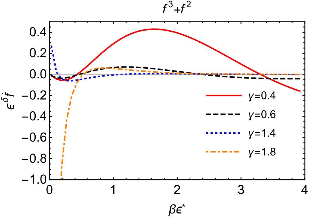 Figure 1
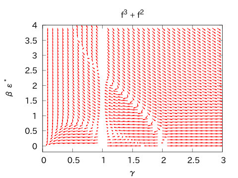 Figure 2
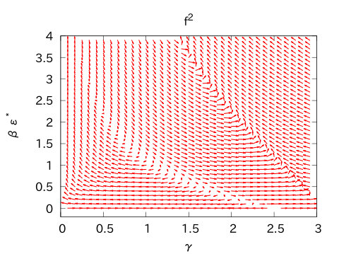 Figure 3
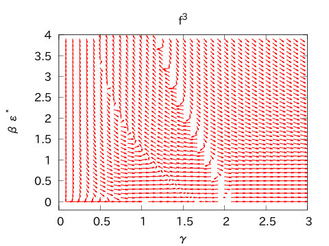 Figure 4
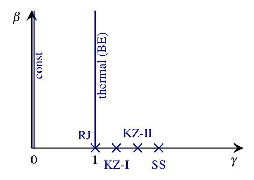 Figure 5
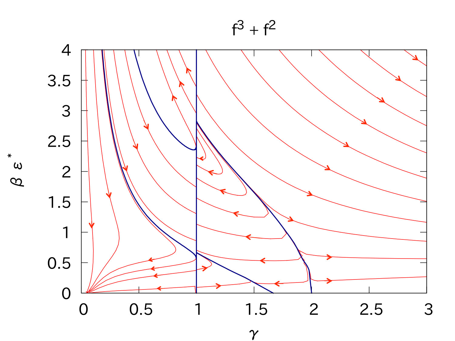 Figure 6
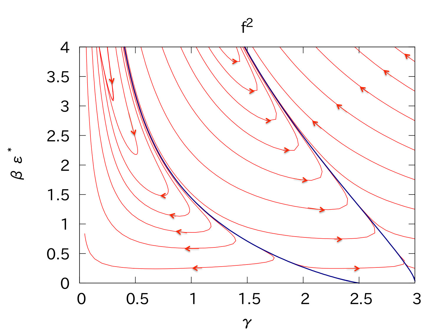 Figure 7
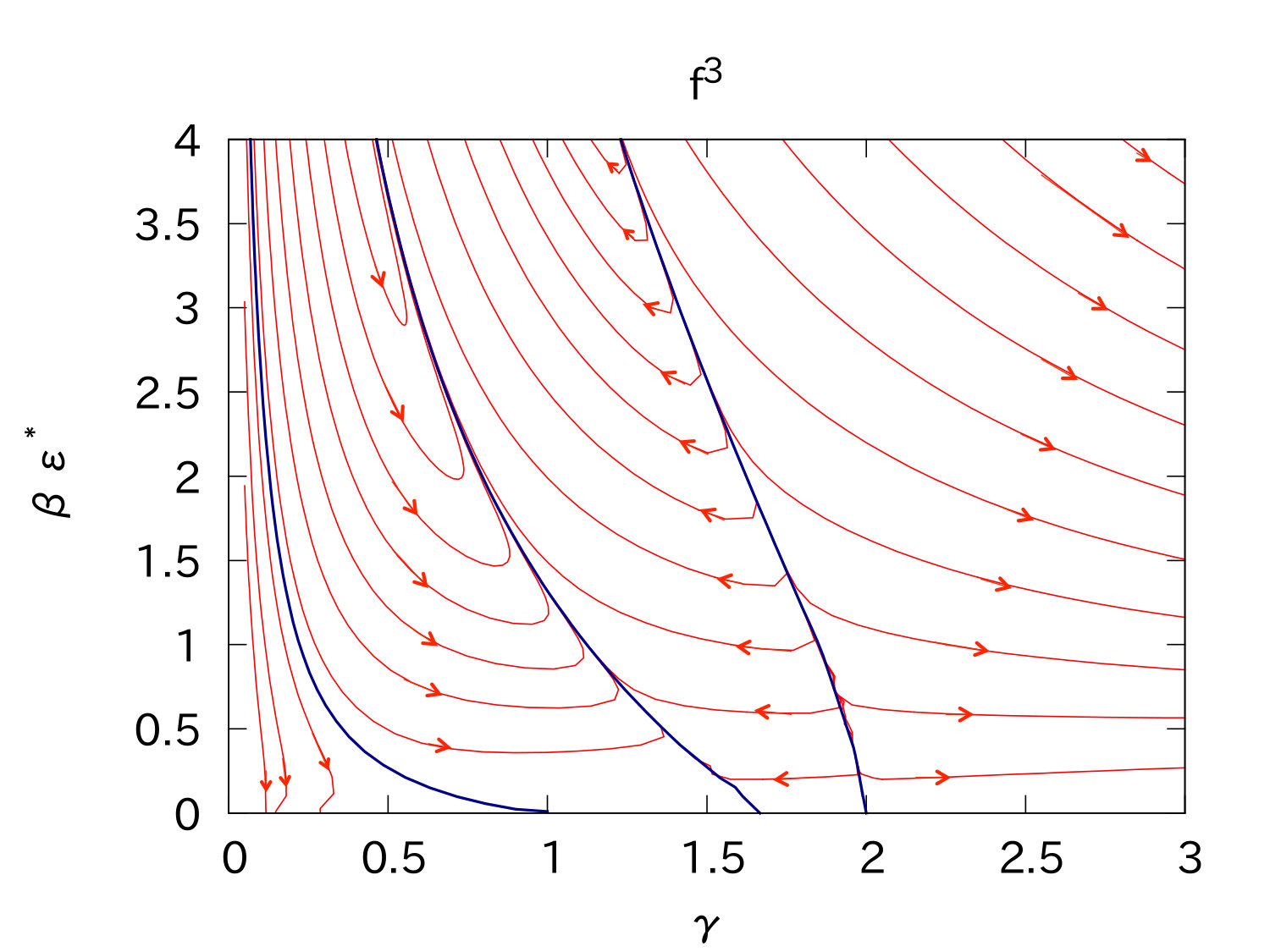 Figure 8
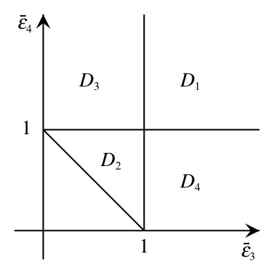 Figure 9
| -regime | -regime | ||
|---|---|---|---|
| Reduced Solution | , | Reduced Solution | , |
| SS , KZ-I | SS , KZ-I | ||
| SS , KZ-II | SS , KZ-II | ||
| SS , RJ | |||
| -regime / -regime | Indices |
|---|---|
| RJ / SS | |
| KZ-I / SS | |
| KZ-II / SS | |
| SS / KZ-I | |
| SS / KZ-II | |
| RJ,KZ-II / KZ-I | |
| RJ / KZ-II | |
| KZ-I / KZ-II |
Peer Reviews
No public reviews on file for this paper yet. If you reviewed it on a platform where reviews are public (OpenReview, ICLR, NeurIPS, ICML), you can paste yours below so the community can read it here.
Videos
No videos yet. Explain this paper in a talk, walkthrough, or lecture? Add one.
Fixed points and flow analysis on off-equilibrium dynamics
in the boson Boltzmann equation
Kenji Fukushima
Koichi Murase
Shi Pu
Department of Physics, The University of Tokyo, 7-3-1 Hongo, Bunkyo-ku, Tokyo 113-0033, Japan
Abstract
We consider fixed points of steady solutions and flow directions using the boson Boltzmann equation that is a one-dimensionally reduced kinetic equation after the angular integration. With an elastic collision integral of the two-to-two scattering process, in the dense (dilute) regime where the distribution function is large (small), the boson Boltzmann equation has approximate fixed points with a power-law spectrum in addition to the thermal distribution function. We argue that the power-law fixed point can be exact in special cases. We elaborate a graphical presentation to display evolving flow directions similarly to the renormalization group flow, which explicitly exhibits how fixed points are connected and parameter space is separated by critical lines. We discuss that such a flow diagram contains useful information on thermalization processes out of equilibrium.
I Introduction
Understanding thermalization dynamics in quantum systems is a long-standing and yet unresolved problem. Even with modern computer advances, solving the first-principle quantum field theories numerically in Minkowskian spacetime demands not only enormous computing resource but also algorithmic innovations. We thus need to assume a reduction of full quantum dynamics in some particular regimes according to our interested problems. In the dilute regime the most useful and widely adopted approach is the Boltzmann equation that can be in principle derived as a quasi-particle approximation of the full quantum equation of motion, i.e. the Kadanoff-Baym or 2PI equation KB ; Cornwall:1974vz (see Refs. Blaizot:2001nr ; Berges:2004yj for comprehensive reviews).
In the context of the relativistic heavy-ion collision (see Ref. Fukushima:2016xgg for a recent review on early thermalization problems), with help from the Boltzmann equation for gluon interactions, the thermalization time scale has been estimated parametrically in terms of the strong coupling constant and the momentum scale that characterizes the initial condition. In this way, the bottom-up thermalization scenario has been established Baier:2000sb , which is further refined later in Refs. Kurkela:2011ti ; Blaizot:2011xf , and is still continued to recent works Kurkela:2015qoa . In fact, since the very early days of the heavy-ion collision physics, the Boltzmann equations has been the common theoretical tool for the investigation of isotropization and thermalization, as pioneered in Ref. Baym:1984np in the relaxation-time approximation and in Ref. Mueller:1999pi with gluon-gluon scattering. We note that a conjecture on a transient formation of the Bose-Einstein condensate Blaizot:2011xf inspired many numerical simulations under an overpopulated condition Berges:2012us ; Xu:2014ega , which may be significantly affected by full interaction dynamics Huang:2013lia ; Berges:2016nru ; Blaizot:2016iir .
In the dense regime, the collision integral in the Boltzmann equation involves higher order scattering processes, and it would make more sense to solve the time evolution in terms of not particles but fields. Recent years, we have witnessed significant developments in a method called the classical statistical simulation (CSS). The CSS is a semi-classical approximation to deal with quantum time evolution. In fact, the Yang-Mills theory, that governs the fundamental laws of gluon interactions, has rich (chaotic) contents even on the classical level as discussed in Ref. Biro:1993qc . Later, in Ref. Arnold:2005ef , by solving the classical Yang-Mills theory coupled with Vlasov equation (i.e. electromagnetic coupled Boltzmann equation), the numerical results imply that a possible turbulent-like energy cascade may help isotropization in weakly coupled non-Abelian plasmas, which is a numerical demonstration of the Chromo-Weibel instability scenario Mrowczynski:1988dz ; Arnold:2003rq (see also Refs. Rebhan:2004ur ; Rebhan:2005re for semi-analytical treatments of the non-Abelian plasma instabilities). The energy decay with similar power-law behavior has been discussed in Ref. Ipp:2010uy , and see also Ref. Fukushima:2013dma for transverse structure formation as well as the longitudinal power-law. Alternatively, in Ref. Mueller:2006up , a different type of power-law in the energy decay has been suggested for non-Abelian plasmas. Now, we should note that a longitudinally expanding case has been studied intensively Attems:2012js ; Berges:2013eia , which generally tends to hinder isotropization.
Interestingly, in high-energy reactions, as a result of small-x evolution of the parton distribution functions, the classical treatment would be a good approximation, and the theoretical framework is well founded under the name of the Color Glass Condensate (CGC) (see Refs. Gelis:2010nm ; Blaizot:2016qgz for reviews). Then, an instability has been discovered once the CGC coherent fields are disturbed by quantum fluctuations Romatschke:2005pm (see also Ref. Berges:2004ce for a related attempt to explain early thermalization in the heavy-ion collision), which motivated systematic investigations on the real-time Yang-Mills dynamics and led to a clear recognition of non-Abelian wave turbulence Berges:2008mr ; Berges:2013eia , where the “turbulence” refers to a power-law spectrum with a certain value of exponent Micha:2004bv . Actually, the theoretical description of the CSS is equivalent to what is called the non-linear Schrödinger equation, which is frequently used in the context of the wave turbulence nazarenko2011wave . Theoretically speaking the exponent of the power-law spectrum may not be unique but take different values depending on microscopic processes. The typical values of exponents correspond to the particle cascade and the energy cascade. It is also possible to anticipate an even larger exponent Carrington:2010sz , and this concept of non-thermal steady states is generalized as the non-thermal “fixed point” in analogy to the Wilsonian renormalization-group (RG) flow. For a review on the non-thermal fixed point and scaling solutions, see Ref. Nowak:2013juc . In a similar sense to the RG analysis, the universality has been pursued numerically Berges:2013fga ; Berges:2014bba , and also the scaling law relations among critical exponents have been investigated Berges:2015ixa . All these recent progresses are very nicely summarized in a lecture note Berges:2015kfa .
We note that the CSS has been highly elaborated and the Wigner distribution function that encodes the initial fluctuations has been determined for expanding geometries Fukushima:2006ax ; Dusling:2011rz . The precise form of the Wigner distribution function is crucial to reproduce the perturbative results correctly, as argued to recover the Schwinger mechanism formula Gelis:2013oca . Then, one would be naturally led to an idea that the CSS with the correct Wigner distribution may already capture the Boltzmann dynamics and may achieve isotropization and thermalization Gelis:2013rba . In fact, there are theoretical discussions on the relation between the Boltzmann equation and the classical field equation Mueller:2002gd ; Jeon:2004dh . As long as the distribution function is large enough to satisfy , these two equations could describe the same physics equivalently. Therefore, in this way, the Boltzmann study with can give an intuitive explanation for some features in the CSS results Epelbaum:2014mfa . One might think that immediately implies that higher order scattering processes should take part in the collision integral. As we will discuss later, however, there exists a certain coupling window in which but the lowest scattering process is still dominant in the collision integral.
If we consider the simplest elastic scattering and drop assuming , the Boltzmann equation with such a truncation has multiple power-law fixed points, one of which corresponds to the Rayleigh-Jeans approximated thermal distribution. If we in turn drop in a dilute regime of , the Boltzmann equation again accommodates several power-law fixed points. The genuine quantum Bose-Einstein distribution function is the asymptotic solution only with a combination of both and . The goal of this paper is twofold. The first is to make a complete classification list of the fixed points or the steady solutions in such truncated Boltzmann equations in the dense and the dilute regimes (see Ref. Mehtar-Tani:2016bay for similar analysis). The second is to clarify the relevance of these fixed points in the full quantum case with and (see Ref. Epelbaum:2015vxa for a closely related work with a similar motivation). For the latter purpose we will propose a new graphical representation of our results in such a way that resembles the RG flows with fixed points and critical lines. The great advantages of such a representation include; (1) intuitively understandable in analogy to the RG flow, (2) clear to judge whether the fixed points are attractive or repulsive, and (3) providing information on critical lines. In particular, we would emphasize that the recognition of the critical lines is regarded as a novelty in our present work, though it is a natural anticipation from the RG analogue.
This paper is organized as follows: In Sec. II we make an overview of the Boltzmann equation, especially one-dimensionally reduced one after the angular integration. Such a simplified representation of the Boltzmann equation is specifically referred to as the boson Boltzmann equation in the literature. We then proceed to the classification of the approximate fixed points or steady solutions in Sec. III. We will there find not only the power-law solutions belonging to the Kolmogorov-Zakharov (KZ) scaling, but also a new self-similar solution. In Sec. IV we present our central results in a form of the flow diagram. We make clear the structure of distinct fixed points and critical lines. Section V is devoted to the conclusion. We note that we set for notational brevity.
II Boson Boltzmann equation
We start with the ordinary Boltzmann equation,
[TABLE]
where is the distribution function for particle with its momentum or energy . The particle velocity and the external force are denoted by and , respectively, and represents the particle scattering effects, which is called the collision integral. For weakly interacting systems we can take account of the collision integral perturbatively, and the elastic scattering at the lowest non-trivial order is the two particle process, namely, the scattering. At this order the collision integral generally reads:
[TABLE]
with particles , , and . In the above expression represents the probability for the scattering process from initial state particles to final state particles within the phase space . We can express the probability using the scattering amplitude as
[TABLE]
In this work we assume spatial homogeneity for the distribution function to drop dependence hereafter. We also consider a special case with spherically symmetric momentum dependence, i.e. the interaction has no angular preference. This is the case for the quartic vertex in the scalar theory, for example. Thanks to the symmetry, the kinetic equation simplifies to be one-dimensional, which not only reduces the computational costs but also resolves the subtle ambiguity on the energy-momentum conservation for discretized momenta.
The symmetry requires that and would be in general a function of momentum modulus. We will, however, introduce the density of states later, and without loss of generality, we can take it as just a constant, i.e., . Thus, we can carry out the angular integration in and the Boltzmann equation (1) takes a simple form, which is often referred to as the boson Boltzmann equation (for this Ref. Markowich2005 contains a short review), that is written as
[TABLE]
where we defined the density of states per space volume PhysRevA.56.575 from
[TABLE]
The simplified collision integral is a function of as follows:
[TABLE]
where in the latter part with the first term represents a process of particles and scattering into particles and , and the second term is the inverse process from and into and . The interaction kernel in our modeling convention is parametrized as
[TABLE]
with . The above form is typical in theoretical models such as the theory (see Refs. Semikoz:1995rd ; Berges:2015kfa for examples). We note that is a constant associated with the density of states (and the momentum dependence in the amplitude). For the relativistic case, Mehtar-Tani:2016bay , while for the non-relativistic case in the denominator of the phase space volume is replaced with the mass , which leads to PhysRevA.53.381 ; Semikoz:1995rd . We give more detailed discussions on and in Appendix A.
III Fixed points
The thermal distribution function should be the final destination of the time evolution in the boson Boltzmann equation. This is the literal definition of “thermalization” and our central interest is to clarify possible paths toward thermalization which would be substantially affected by the structures of other fixed points and flow patterns connecting or disconnecting them.
In numerical simulations power-law spectra have been found as transient states on the way toward thermalization, and thus, for theoretical characterization of thermalization, it would be the most essential first step to understand those power-law spectra as much analytically as possible. For such analytical treatments the boson Boltzmann equation provides us with a useful framework. It is much simpler than the original Boltzmann equation, and nevertheless, it still encompasses a variety of steady solutions. We shall first summarize these analytical solutions in what follows below.
In this paper we limit ourselves to the scattering in the collision integral, and then discuss two approximated forms in extreme regimes as well as the full quantum one in Eq. (6).
The first extreme is the dense regime or we will call it the -regime in this paper. In a kinetic region where is larger than the unity, terms become dominant over terms in the collision integral (6). One may think that more and more particles would be involved in the collision integral for , but there is a certain kinetic window in which is compatible with the truncation up to the process. This is the case for
[TABLE]
that holds at sufficiently weak coupling. Then, in the -regime, the kinetic equation is approximated as
[TABLE]
where .
Another extreme is the dilute regime or we will call it the -regime. If the momentum or energy is sufficiently large, the distribution function should generally get smaller and eventually we come to the kinematic regime where
[TABLE]
Then, the kinetic equation in the -regime is approximated as
[TABLE]
In the subsequent subsections we will consider the steady solutions for Eqs. (9) and (11).
III.1 Thermal distribution
It is well understood that the detailed balance is satisfied for the thermal distribution function. That is, we can readily confirm that the thermal distribution function makes vanishing. For the full quantum case with both and terms, we can find the solution from the famous theorem as
[TABLE]
where two parameters in the above Bose-Einstein distribution, and , represent the temperature inverse and the chemical potential, which dynamically depends on the choice of at .
In the -regime, we can use the theorem in the same way Epelbaum:2014mfa to find a thermal fixed point,
[TABLE]
This is nothing but a Rayleigh-Jeans approximated form of the Planck spectrum (12) for . Indeed, in this region for , the Bose-Einstein distribution is infrared enhanced, so that as they should be in the -regime.
In the -regime, on the other hand, it is again immediate to find a thermal fixed point as given by
[TABLE]
This is the Maxwell-Boltzmann distribution in classical physics, that is again a natural consequence from the fact that quantum effects are negligible for dilute systems. Here, let us make a remark on the usage of the word, “classical”, which is sometimes confusing in the literature. Usually is often referred to as classical in a sense that this is a solution in the -regime where the semi-classical approximation works. In fact, the CSS using the classical equation of motion would lead to this power-law form of the thermal spectrum. Also, is of course a classical distribution in a conventional sense of statistical mechanics.
We point out that there is always another solution that satisfies the detailed balance, that is the constant solution given by
[TABLE]
This makes vanishing in all the -regime, the -regime, and the full quantum regime. The physical meaning is obvious; this is a trivial solution in the limit, and the integrated total energy and particle number are ill-defined. Thus, such a constant solution has no physical significance. In later discussions on the flow diagram, however, we should be aware of the existence of this solution in order to understand the flow structures.
III.2 Kolmogorov-Zakharov spectra
It is interesting to see that the kinetic equations in the -regime and the -regime, Eqs. (9) and (11), respectively, accommodate more non-trivial steady solutions than the thermal distribution. Such solutions of the power-law form are commonly called the Kolmogorov-Zakharov (KZ) spectra, which are generally power-law spectra characterized by exponents kolmogorov1941local ; zakharov1967weak ; zakharov1972collapse . For the KZ solutions the collision integral becomes zero not due to the detailed balance. The gain and the loss from the higher energy region and the lower energy region cancel out, which makes the collision integral vanishing. Although it is already an established method, it would be instructive to make a quick review of the Zakharov conformal transformation that is a mathematical trick to reverse the higher/lower energy regions in a specific conformal way.
For the moment, as the following discussions can be applied to both the -regime and the -regime, let us write the collision integral in a generic form as
[TABLE]
where in the full quantum case, in the -regime, and in the -regime.
Because of the delta function, the integration is easily done to substitute . Let us now introduce dimensionless variables, , and then the collision integral reads,
[TABLE]
where with . The dimensionless integrand is defined as . The integration region with respect to and is split into four domains () as shown in Fig. 1. We note that the region for is excluded because this region does not meet the energy conservation.
The Zakharov transformation is a conformal mapping among the domains . We shall pick up one example. For the integration over , we can change the integration variables as and , where so that the energy conservation is consistent also for with . Then, in the region, by definition, , and a factor arises from the integration measure (note that is a function of and ). Most importantly, the allowed region for and coincides with , i.e. and . Therefore, we have,
[TABLE]
where we inserted (instead of the unity) for a symmetric representation. Similarly, we can change the variables according to respective regions of as summarized below:
[TABLE]
The top on the table is the transformation as seen in Eq. (18). The second and the third transformations introduce and in such a way that the allowed region for them becomes . In this way, adding the original integration in the domain (for which, and can be safely inserted), we can find the collision integral transformed in the following way in the domain only:
[TABLE]
This expression is valid for any form of distribution function and its functional as far as the original integration in each domain is convergent.
Now we shall find the KZ solutions of the form, , with which the collision integral vanishes. The KZ solutions can exist if has the scaling property,
[TABLE]
for an arbitrary number and an index fixed by , and if has the symmetry under particle exchanges,
[TABLE]
Using the symmetries we can reorganize the integral as
[TABLE]
It is clear from the above expression that either or makes , for which the underlying mechanisms are to be identified as the particle number conservation and the energy conservation, respectively Mehtar-Tani:2016bay . These relations lead to the following KZ exponents,
[TABLE]
In the present work we will call these two solutions the KZ-I and the KZ-II, respectively.
In the -regime with Eq. (9) the index is , and then more explicit forms of the KZ-I and the KZ-II solutions read,
[TABLE]
The KZ-I and KZ-II solutions correspond to the particle and the energy flow, respectively, as we already mentioned above when we derived .
In the -regime with the index , the KZ-I and the KZ-II solutions are given, respectively, as
[TABLE]
III.3 Self-similar evolving solution
We address a new type of solution in the -regime and also the -regime, that is not a steady solution like the KZ spectra, but a scaling solution having explicit time dependence. We name it the self-similar (SS) evolving solution. The SS solution appears as
[TABLE]
where is a constant, and is an index characterizing the density of states as . The coefficient is given by
[TABLE]
Here, in the above expression, a specific power-law functional form is substituted for , and after the , , integrations in , we get rid of by taking it to be the unity. That is, represents the coefficient apart from the energy dependent part.
Let us explain how to find this SS solution in more details. To this end, we introduce an Ansatz, . Then, the left-hand side of the kinetic equation becomes,
[TABLE]
Again, here, we note that represents the coefficient apart from and the mass dimension is not skewed up. The right-hand side is,
[TABLE]
By equating above expressions, we readily find the following choice of and is sufficient:
[TABLE]
For special combinations of and , the SS solution is reduced to the KZ or the RJ solutions. In such cases, is the exponent of the KZ/RJ solutions and vanishes so that is constant. Such combinations of and corresponding to reduced solutions are summarized in Table 1.
III.4 Intersection of solutions
For the full quantum case including both and terms as in Eq. (6), there is in general no scaling solution of the form, . Nevertheless, for special values of the indices, and , we find that an SS solution in the -regime and the -regime becomes an analytically exact solution for the full quantum case. This is the case typically for indices that allow for some scaling solutions in the -regime and the -regime simultaneously.
Such special indices are summarized in Table 2 together with the solutions in the -regime and the -regime, as well as physically unaccepted solutions.
On Table 2 the first three are physically possible, for which the SS solution in the -regime intersects with the power-law solutions in the -regime, so that the solution can satisfy the full kinetic equation. For , that is unlikely in physical systems, the SS solution in the -regime intersects with the power-law solutions in the -regime, as listed on the 4th and 5th lines in Table 2. Logically speaking, there are combinations of indices that make the KZ solutions possible in the -regime and the -regime at the same time. Then, however, as listed on the last three lines in Table 2, which leads to infrared divergent and is not physically acceptable.
IV Numerical results and flow diagram
We shall now proceed to the numerical calculations to solve the boson Boltzmann equation. Because it is one-dimensionally reduced, it is quite easy to solve the boson Boltzmann equation even in a brute-force numerical way, and moreover, there is no subtlety in implementing the energy-momentum conservation on the phase-space grid. We could have shown many numerical results for whole time evolution with various initial conditions, but such presentations would not be illuminating to deepen our understanding on general dynamics out of equilibrium. We will thus first develop a new analysis to extract the information inspired by the (perturbative) RG study. Then, after making a remark on the convergence of the collision integral that limits the sensible parameter range, we will show the flow diagrams and discuss the physical meaning of the critical lines.
IV.1 Method
To restrict our consideration within finite dimensional parameter space, we here introduce three parameters, , , and , to parametrize the distribution function as follows:
[TABLE]
This parametrized Ansatz can encompass all kinds of solutions as we have seen so far. The choice of makes reduced to the standard Bose-Einstein distribution function. It should be noted that and then have the ordinary interpretation as the inverse temperature and the chemical potential, respectively. The limit of makes constant and then and are completely irrelevant.
The -regime for is realized in the low energy region where . In this region has the asymptotic form given by , which is compatible to the RJ/KZ/SS solutions in the -regime if . In the -regime corresponding to the high energy region of , the function correctly reproduces the Maxwell-Boltzmann distribution, .
If we are interested in the possibility of the Bose-Einstein condensation, we should deal with non-zero , but we can set for the present work. Then, all the fixed points as discussed so far are located on - plane as schematically illustrated in Fig. 2.
Now we are interested in the time evolution of and on top of these fixed points. Strictly speaking, the full time evolution of cannot be completely captured by only two parameters in Eq. (32). In this sense, our approach somehow shares the truncation scheme with the perturbative RG flow analysis, for which the functional space is restricted to the one described by a finite number of couplings.
What we are doing is the following. We will compute the time derivatives of and at each point (,) to show the vector that represents the flow direction at that point. We also implicitly assume looking at a narrow energy window around . Then, the local shape of the distribution function is well approximated by its local value and derivative, and , with . Now, to shorten the notation, let us denote the energy differentiated as . For an infinitesimal time increase, the time evolution of the distribution function is also approximated by local quantities differentiated with respect to the time, i.e. and . We can numerically obtain these time derivatives from the collision integral. We make a remark that it is convenient to employ the Zakharov transformed expression (19) for the numerical integration because it guarantees the exact numerical cancellation in the collision integral at the KZ fixed points.
Then, we need to evaluate and from . The idea is that and should best reproduce the shape of (non-truncated) . Up to the first order in terms of the energy derivatives, the following matrix equation must hold:
[TABLE]
Here, we notice that this matrix form can be trivially extended for a larger number of parameters by taking account of the higher order energy derivatives.
The vector field, , makes our “flow” diagram associated with the kinetic equation. More details on our concrete numerical procedures are explained in Appendix B. The flow diagram enables us to discuss the global structure of the time evolution of the kinetic equation as discussed in Sec. IV.3.
IV.2 Convergence of collision integral
Before we turn to discuss our numerical results, we will briefly discuss the validity region of our analysis in parameter space. Since the original collision integral has some parameter space without absolute convergence, the flow results there should not be trustable even though the behavior seems non-singular. Thus, it is important to quantify the convergence condition for the collision integral.
For the numerical integration of the collision integral, we adopt the expression (19) after the Zakharov transformation, which chooses a specific combination of the integration domains. Even when a regular output results from our analysis, therefore, it does not necessarily describe physically sensible behavior unless the original collision integral converges.
Since for , the fitting function is no longer positive definite then. So we should first require . To guarantee the ultraviolet convergence, we should next require . Let us see below how the infrared properties further constrain allowed . As a matter of fact, because the distribution function has an approximate power form in the infrared region, a larger would suffer a stronger infrared singularity. Here, we note that, though we could analyze the collision integral (16) directly, it would be easier to start with the expression (19) after the Zakharov transformation, with which original “infrared” divergences in Eq. (16) are transformed into “ultraviolet” divergences in Eq. (19). It should be noticed that we need to evaluate each term in Eq. (19) separately to check the absolute convergence of the original collision integral. There are two possible situations having divergences. One is the case that either or gets infinity. The other possibility is the case that both and get infinity. We obtain two different power-law behaviors with respect to an ultraviolet cut-off corresponding to these two situations. By reading the exponents of the power-law behaviors, we can quantitatively identify the validity regions.
In the -regime, the collision integral, whose explicit form appears in Eq. (11), yields . For the convergence, the power of such dependence should be non-positive, that is,
[TABLE]
In the -regime, when with being finite, the collision integral (9) behaves as . If both and approach , the collision integral is . As long as , the former condition is stronger than the latter and is constrained as
[TABLE]
For the full quantum case with and terms in the collision integral, the convergence condition follows from the stronger one of above two limiting cases. For example, for , the condition in the -regime is and that in the -regime is , so that the condition in the full dynamics is given by the latter () that is stronger than the former ().
IV.3 Flow diagrams
Our main results of the flow diagrams are summarized in Figs. 3, 4, and 5 for the -regime with Eq. (9), the -regime with Eq. (11), and the full quantum case with Eq. (6), respectively. In the present work we chose (there is no particular reason for this choice). To draw figures we took for the horizontal axis and for the vertical axis; in our Ansatz, only a product of appears. Thus, to draw these figures, we changed with the energy fixed at . For the graphical representation we rescaled the length of the vector from to where we chose and , , and for the full quantum case, the -regime, and the -regime, respectively, with defined. We note that Fig. 5 does not show points for and because of slow convergence of the numerical calculation.
On these flow diagrams we anticipate that fixed points should manifest themselves as points where the flows stop. In fact, we can easily see such points on these flow diagrams in accord with discussions and a schematic picture given in Sec. III.
In the -regime, we can locate three fixed points precisely corresponding to power-law solutions on the horizontal axis (on ): the RJ (), the KZ-I (), and the KZ-II () solutions on Fig. 3. In the -regime, on Fig. 4, there appear two fixed points: the KZ-I () and the KZ-II () solutions.
For the full quantum case, that is of our main interest, we can find the Bose-Einstein solutions at with various temperatures along the vertical line on Fig. 5. We can see the power-law solutions of the -regime near and also in this case with the full quantum terms. This is because the occupation number becomes large near the horizontal axis , so that the full quantum equation (6) is effectively reduced to that of the -regime (9).
The most remarkable feature on these flow diagrams is not the manifestation of the fixed points, but the flow pattern around the fixed points. Actually we see that the flow directions form several distinct regions, with which the whole parameter space is split into different “phases” that is again reminiscent of the perturbative RG flow diagram. Interestingly, for each power-law solution, as seen in Figs. 3 and 4, one “line” with rapid change of the flow directions is always attached to one fixed point, which defines the borders of phases. Moreover, in the full quantum case as in Fig. 5, those lines are crossed with the thermal line at to shape a more complicated phase structure. In the next subsection we discuss these lines more closely.
IV.4 Flow lines and phase boundaries
To make the phase structure visible more prominently, and to understand how the fixed points are connected by phase boundaries, it would be very useful to consider “flow lines” on the diagrams as shown in Figs. 6-8. Instead of the vector field as discussed in Sec. IV.3, we would pay our attention to their integral curves, which we call the “flow lines” throughout this paper. We can identify the flow lines by solving the following set of equations using the Runge-Kutta 3/8-rule, i.e. one of the order methods:
[TABLE]
where is a parameter along the curve. In Figs. 6-8 we show flow lines by red lines together with supplementary arrows indicating the flow directions. It should be noted that initial points are chosen by hand arbitrarily.
Although the precise locations of respective flow lines are irrelevant, it is physically meaningful where the phase “boundaries” appear, which are shown by blue lines on Figs. 6-8. The most trivially understandable phase boundary is the thermal line at in the full quantum case in Fig. 8. It is also clear that the flow line starting from the KZ-I point is an attractive line in the full quantum case as well as in the -regime in Fig. 6; surrounding flow lines around the boundary run in the direction approaching the attractive line. In contrast, the flow line starting from the KZ-II point is a repulsive line, i.e. flow lines branch out from this unstable repulsive line. In the -regime, similarly, the boundary starting from the KZ-I (and KZ-II) point is a repulsive (and attractive, respectively) line.
We point out that there is another kind of phase boundary in the region in the full quantum case as noticed in Fig. 8. This region is further divided by two phase boundaries into three distinct phases according to the final destinations of the flow. The destination in the small phase is the origin on the diagram which corresponds to a constant solution. The destination in the middle phase is the thermal line. In the large phase, the flow tends to go to . We note that these structures share features seen also in the -regime in Fig. 6.
IV.5 More discussions
Here we take a closer look at the flow diagrams and discuss the implications to the real-time dynamics. We shall consider only the full quantum case in Fig. 5 in this subsection, but the generalization of the interpretations for Figs. 3 and 4 is straightforward.
In the following discussion let us regard as a changeable variable rather than . This implies that, for a given , we can obtain qualitative information on the time evolution of the whole distribution function by looking at the flow pattern on the diagram.
In Fig. 4 we notice that the vectors have the opposite signs in the left and the right sides from the line at . To discuss underlying physics for such different behavior, we divide the flow diagram into three regions: the region-I refers to , the region-II refers to , and the region-III refers to . We should remember that, as already mentioned in Sec. IV.2, makes the collision integral non-convergent, and thus, we should exclude this region from our consideration. In order to explain the flow diagram better, we make plots for the collision integral as a function of for various values of in Fig. 9.
For (region-I), from Fig. 9, we see that at small and large energies is negative, and so in these energy regions should decrease. In the middle energy region is positive and the system accumulates more particles in this middle energy region.
Because the distribution function naturally flows toward thermalization, we can anticipate that more and more particles will be transferred from large to small through interactions. In fact, to satisfy the particle number conservation and the energy conservation simultaneously, a particle at very large must interact with a particle at very small , turning into a positive contribution to a particle at middle . This is an intuitive explanation for the observation that is negative at small and large energies, while it is positive in the middle energy region in Fig. 9.
Now, let us take a turn back to the flow diagram of Fig. 5. For large , the flow is directed from high energy to low energy, while the flow changes its direction around . As is clear in Fig. 5, for , the direction of flow is almost parallel to the -axis, that means the energy is hardly changed along the flow though the number of soft particles increases. Actually, is a special point that makes our Ansatz (32) as simple as regardless of . Therefore, the sensitivity of becomes far stronger then and the flow should be almost parallel to the -axis.
For (region-II), the collision integral is positive for small only as shown by the blue dotted line in Fig. 9. We argue that the system tends to reach the KZ-I solution rather than moving straight to thermal equilibrium, which accounts for the observation that the system will accumulate more soft particles only. Turning back to the flow diagram in Fig. 5, we see that the flow is again approximately parallel to the -axis in small region. Along the flow gets larger as the time goes, and this means that the number of soft particles increases. Then, for larger the flow pattern changes and becomes similar to the one in the region-I with small . For further larger , the flow behavior is just the same as that in the region-I.
For (region-III), the flow pattern looks similar to that in the region-I at middle energy, and the underlying physic is similar. In the small region the system is over-populated especially near the KZ-II solution. Then, since we have not considered a possible condensate (with entirely) in our analysis, the particle number conservation does not allow soft particles to increase. As a results, the system will accumulate more particles in the middle energy region only. That is the reason why the region-III exhibits some similarity to the region-I.
V Conclusion
In this work we classified various non-trivial fixed points in space of the distribution function described by the boson Boltzmann equation. We proposed a new graphical way to analyze the dynamical structures, i.e. the flow diagrams and the phase diagrams resulting from the boson Boltzmann equation. For bosonic systems the most well-known thermal fixed point is the Bose-Einstein (BE) distribution, that is a solution satisfying the detailed balance with quantum terms in the collision integral. In the lowest order scattering, the full collision integral contains terms involving both and . In the dense limit which we call the -regime in this work, the collision integral keeps only the terms, leading to the Rayleigh-Jeans (RJ) approximated form of the thermal distribution function. In the dilute limit or the -regime, on the other hand, the collision integral is truncated only with the terms and the thermal distribution is approximated by the Maxwell-Boltzmann (MB) form. In the / regimes there are additional non-trivial solutions of the boson Boltzmann equation: Two Kolmogorov-Zakharov spectra, namely, KZ-I and KZ-II, are non-trivial power-law fixed points corresponding to the particle and the energy cascade, respectively. Furthermore, we addressed a new type of power-law fixed point: We found the self-similar (SS) evolving solutions whose overall factor has explicit time dependence. Interestingly, even in the full quantum case with both the and the terms, there can exist power-law solutions at the interaction of those non-trivial fixed points in the / regimes.
We postulated a parametrization of the distribution function so that thermal fixed points and other non-trivial power-law fixed points are interpolated and mapped into parameter space spanned by . The time evolution of the parameters, , indicates the directions of infinitesimal (quasi-static) temporal changes from the parametrized initial condition, and were numerically obtained from the local time evolution around an energy window . We constructed the flow diagrams by plotting the vector field, , in the two-dimensional plane. We observed a clear manifestation of fixed points corresponding to the thermal distribution, the KZ-I, and the KZ-II solutions on the flow diagram. Besides, we noticed characteristic flow patterns around these fixed points. The whole parameter space is then split into several distinct phases bounded by critical lines, which is intuitively understood in analogy to the perturbative RG flow diagrams. To investigate more clear relations of fixed points and critical lines, we numerically identified the flow lines on the flow diagrams. Our concrete demonstration shows that the clarification of the fixed points, the critical lines, and the flow lines should provide us with useful information on the thermalization processes including transient behavior at intermediate stages. In the full quantum case the flow lines become far complicated with the thermal (BE) critical line that crosses flow lines. The flow diagram also tells us transparently that the critical lines starting from the KZ-I and the KZ-II points are directed with attractive and repulsive behavior, respectively.
As we emphasized, our proposed tools of the RG-like flow diagram offer us an intuitive access to investigate the dynamics out of equilibrium. In the present study one might have thought that our arguments may rely on special setups of the boson Boltzmann equation, the scattering, the Ansatz of the distribution function with , but none of them is a crucial limitation. Because we aimed to exemplify how useful our new analysis is, we employed the simplest setup in the present work. We can almost trivially extend our current treatment to more general systems. With sufficient computational resources, in principle, one can numerically solve the kinetic equation in full phase space, including inelastic and higher-order collisions terms. Such improvements would quantitatively affect , that can be translated into . Rather, depending on the problem of our interest, we need to consider some other types of parametrization of the distribution function. For example, in this work, we reported a new solution of the boson Boltzmann equation called the SS solution, but the Ansatz we adopted was not suitable for confirming it numerically. We tested many other functional forms and, in fact, some of them were capable of seeing the SS solution properties, but they did not have good resolution for other fixed points. The optimal parametrization awaits to be found. Although we did not pay much attention to the SS solution in this paper, its physical implication must be an intriguing problem in the analytical aspect of the Boltzmann equation, which deserves future investigations.
Acknowledgements.
The authors thank François Gelis, Yoshimasa Hidaka, Jinfeng Liao, Yacine Mehtar-Tani for useful discussions and comments. K.F. and K.M. were partially supported by JSPS KAKENHI Grant No. 15H03652 and 15K13479. S.P. was supported by the JSPS Postdoctoral Fellowship for Foreign Researchers.
Appendix A Derivation of Eqs. (6) and (7)
In the relativistic case, , the collision integral in Eq. (2) can be written as,
[TABLE]
where represents the angular part of the phase space integration. For the full quantum process, the interaction involves,
[TABLE]
We can explicitly carry out the angular integration with the delta function constraint as follows,
[TABLE]
Inserting the above to yields,
[TABLE]
where we set assuming a simple interaction like that in the theory. Recalling that the density of states is given as
[TABLE]
we finally get,
[TABLE]
We note that, in the above expression, we absorbed all irrelevant constant factors into a redefinition of .
In the same way we can derive the boson Boltzmann equation for the non-relativistic case. The difference is that the energy dispersion relation is not but . The collision integral then becomes,
[TABLE]
The angular integration is the same as Eq. (39) and the density of states changes as
[TABLE]
After all, we arrive at
[TABLE]
For more general discussions, readers can consult Refs. PhysRevA.56.575 ; PhysRevA.53.381 and, for the mathematical analysis of the collision integral in the Boltzmann equation, see a review escobedo2003 .
Appendix B More details on the numerical procedure
To evaluate the right-hand side of Eq. (33) we utilize the following form of the integrations;
[TABLE]
where the integrand is a function of and with , , , and . For the numerical integration we employed the Gauss-Legendre quadrature. To check the convergence, we compared and order quadratures. Using this integration we can write the right-hand side of Eq. (33) as
[TABLE]
where with . In the -regime, the explicit forms of and are
[TABLE]
where we defined , , and . Likewise, in the -regime, the explicit forms read,
[TABLE]
In the full quantum case, we can just combine expressions in the- regime and the -regime to have,
[TABLE]
We can obtain the matrix elements in the left-hand side of Eq. (33) by taking the differentiation of the fitting function explicitly as
[TABLE]
Finally, here, we notice that the collision integrals in Eqs. (47) and (48) are functions of apart from a common factor . The matrix elements in the left-hand side are also functions of . The common factor, , does not affect the direction of the flow, but only changes its velocity. Therefore, only the dependence is relevant for our analysis on the structure of the flow diagrams.
The reference list from the paper itself. Each links out to its DOI / PubMed record.
- 1(1) L. Kadanoff and G. Baym, Quantum statistical mechanics . Benjamin, New York, 1962.
- 2(2) J. M. Cornwall, R. Jackiw, and E. Tomboulis, “Effective action for composite operators,” Phys. Rev. D 10 (1974) 2428–2445 . · doi ↗
- 3(3) J.-P. Blaizot and E. Iancu, “The Quark gluon plasma: Collective dynamics and hard thermal loops,” Phys. Rept. 359 (2002) 355–528 , ar Xiv:hep-ph/0101103 [hep-ph] . · doi ↗
- 4(4) J. Berges, “Introduction to nonequilibrium quantum field theory,” AIP Conf. Proc. 739 (2005) 3–62 , ar Xiv:hep-ph/0409233 [hep-ph] . · doi ↗
- 5(5) K. Fukushima, “Evolution to the Quark-Gluon Plasma,” Rept. Prog. Phys. 80 no. 2, (2017) 022301 , ar Xiv:1603.02340 [nucl-th] . · doi ↗
- 6(6) R. Baier, A. H. Mueller, D. Schiff, and D. T. Son, “’Bottom up’ thermalization in heavy ion collisions,” Phys. Lett. B 502 (2001) 51–58 , ar Xiv:hep-ph/0009237 [hep-ph] . · doi ↗
- 7(7) A. Kurkela and G. D. Moore, “Thermalization in weakly coupled nonabelian plasmas,” JHEP 12 (2011) 044 , ar Xiv:1107.5050 [hep-ph] . · doi ↗
- 8(8) J.-P. Blaizot, F. Gelis, J.-F. Liao, L. Mc Lerran, and R. Venugopalan, “Bose–Einstein condensation and thermalization of the Quark Gluon Plasma,” Nucl. Phys. A 873 (2012) 68–80 , ar Xiv:1107.5296 [hep-ph] . · doi ↗