Equation of State Based Slip Spring Model for Entangled Polymer Dynamics
Georgios G. Vogiatzis, Grigorios Megariotis, Doros N. Theodorou

TL;DR
This paper introduces a mesoscopic Brownian dynamics model for entangled polymer melts that incorporates an equation of state for accurate nonbonded interactions, enabling predictive simulations of specific polymer systems like cis-1,4-polyisoprene.
Contribution
The paper develops a novel slip spring model based on an equation of state, integrating kinetic Monte Carlo and bottom-up parameter derivation for realistic polymer melt simulations.
Findings
Quantitative predictions of polymer structure and dynamics.
Validation against experimental data for cis-1,4-polyisoprene.
Reproduction of thermodynamics and rheology without fitting.
Abstract
A mesoscopic, mixed particle- and field-based Brownian dynamics methodology for the simulation of entangled polymer melts has been developed. Polymeric beads consist of several Kuhn segments, and their motion is dictated by the Helmholtz energy of the sample, which is a sum of the entropic elasticity of chain strands between beads, slip springs, and nonbonded interactions. The entanglement effect is introduced by the slip springs, which are springs connecting either nonsuccessive beads on the same chain or beads on different polymer chains. The terminal positions of slip springs are altered during the simulation through a kinetic Monte Carlo hopping scheme, with rate-controlled creation/destruction processes for the slip springs at chain ends. The rate constants are consistent with the free energy function employed and satisfy microscopic reversibility at equilibrium. The free energy of…
Click any figure to enlarge with its caption.
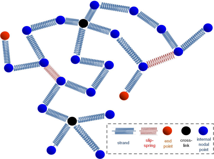 Figure 1
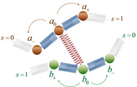 Figure 2
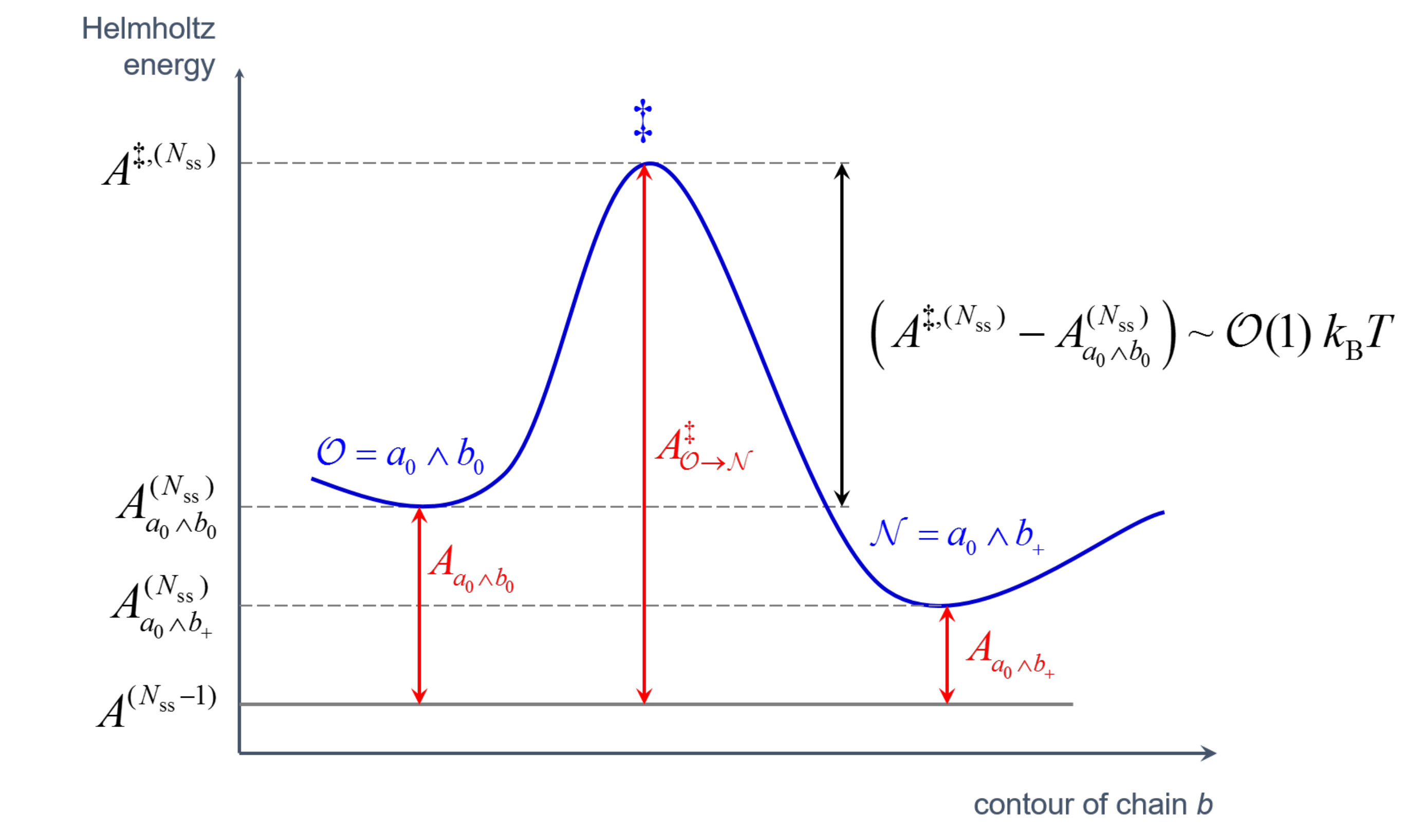 Figure 3
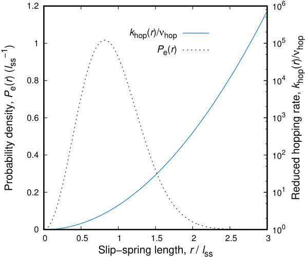 Figure 4
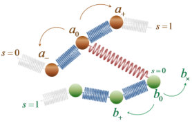 Figure 5
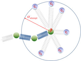 Figure 6
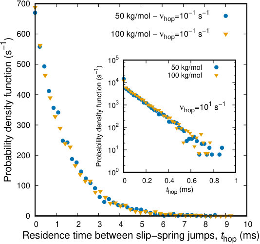 Figure 7
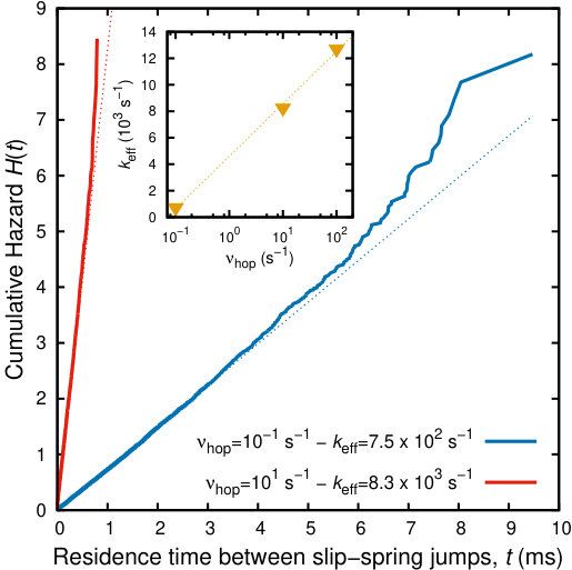 Figure 8
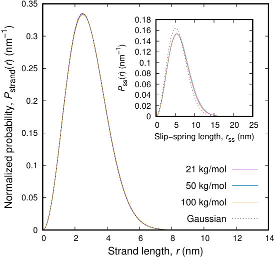 Figure 9
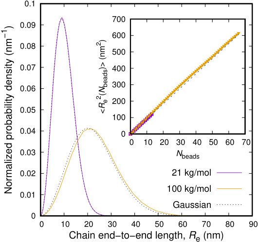 Figure 10
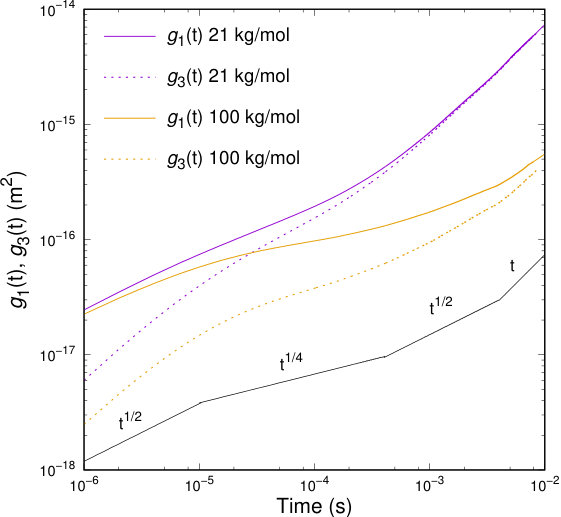 Figure 11
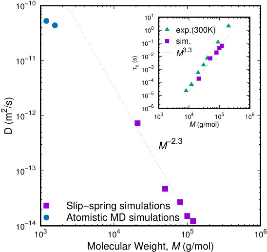 Figure 12
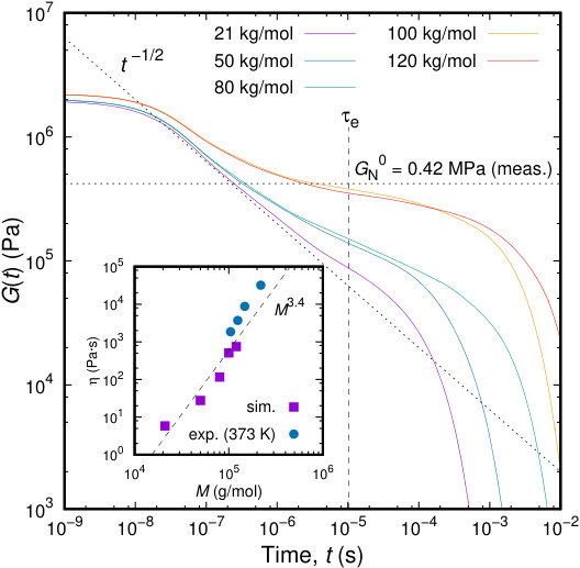 Figure 13
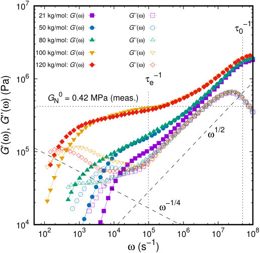 Figure 14
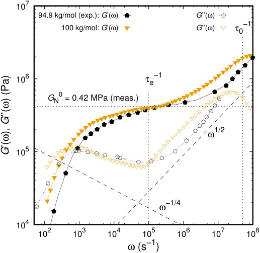 Figure 15
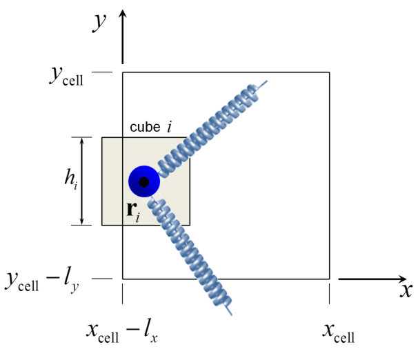 Figure 16
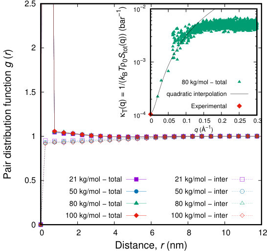 Figure 17
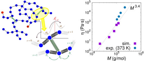 Figure 18
Peer Reviews
No public reviews on file for this paper yet. If you reviewed it on a platform where reviews are public (OpenReview, ICLR, NeurIPS, ICML), you can paste yours below so the community can read it here.
Videos
No videos yet. Explain this paper in a talk, walkthrough, or lecture? Add one.
Equation of State-based Slip-spring Model for Entangled Polymer Dynamics
Georgios G. Vogiatzis
Grigorios Megariotis
Doros N. Theodorou
[
Abstract
A mesoscopic, mixed particle- and field-based Brownian Dynamics methodology for the simulation of entangled polymer melts has been developed. Polymeric beads consist of several Kuhn segments and their motion is dictated by the Helmholtz energy of the sample, which is a sum of the entropic elasticity of chain strands between beads; slip-springs; and non-bonded interactions. Following earlier works in the field (Phys. Rev. Lett. 2012, 109, 148302) the entanglement effect is introduced by the slip-springs, which are springs connecting either non successive beads on the same chain, or beads on different polymer chains. The terminal positions of slip-springs are altered during the simulation through a kinetic Monte Carlo hopping scheme, with rate-controlled creation/destruction processes for the slip-springs at chain ends. The rate constants are consistent with the free energy function employed and satisfy microscopic reversibility at equilibrium. The free energy of nonbonded interactions is derived from an appropriate equation of state and it is computed as a functional of the local density by passing an orthogonal grid through the simulation box; accounting for it is necessary for reproducing the correct compressibility of the polymeric material. Parameters invoked by the mesoscopic model are derived from experimental volumetric and viscosity data or from atomistic Molecular Dynamics simulations, establishing a “bottom-up” predictive framework for conducting slip-spring simulations of polymeric systems of specific chemistry. Initial configurations for the mesoscopic simulations are obtained by further coarse-graining of well-equilibrated structures represented at a greater level of detail. The mesoscopic simulation methodology is implemented for the case of cis-1,4 polyisoprene, whose structure, dynamics, thermodynamics and linear rheology in the melt state are quantitatively predicted and validated without a posteriori fitting the results to experimental measurements.
NTUA]School of Chemical Engineering, National Technical University of Athens, 9 Heroon Polytechniou Street, Zografou Campus, GR-15780 Athens, Greece
1 Introduction
One of the fundamental concepts in the molecular description of structure - property relations of polymer melts is chain entanglement. When macromolecules interpentrate, the term entanglements intends to describe the topological interactions resulting from the uncrossability of chains. The fact that two polymer chains cannot go though each other in the course of their motion changes their dynamical behavior dramatically, without altering their equilibrium properties. Anogiannakis et al.1 have examined microscopically at what level topological constraints can be described as a collective entanglement effect, as in tube model theories, or as certain pairwise uncrossability interactions, as in slip-link models. They employed a novel methodology, which analyzes entanglement constraints into a complete set of pairwise interactions (links), characterized by a spectrum of confinement strengths. As a measure of the entanglement strength, these authors used the fraction of time for which the links are active. The confinement was found to be mainly imposed by the strongest links. The weak, trapped, uncrossability interactions cannot contribute to the low frequency modulus of an elastomer, or the plateau modulus of a melt.
In tube model theories,2, 3, 4, 5 it is postulated that the entanglements generate a confining mean field potential, which restricts the lateral monomer motion to a tube-like region surrounding each chain. In polymer melts the confinement is not permanent, but leads to a one- dimensional diffusion of the chain along its tube, called reptation.6 An alternative, discrete, localized version of the tube constraint is utilized in models employing slip-links. 7, 8, 9, 10, 11, 12, 13 The tube is replaced by a set of slip-links along the chain, which restrict lateral motion but permit chain sliding through them. The real chain is represented by its primitive path, which is a series of strands of average molar mass connecting the links.
Hua and Schieber11, 12 considered that the molecular details on the monomer or Kuhn-length level are smeared out in the slip-link model, while the segmental network of generic polymers is directly modeled, by introducing links between chains, which constrain the motion of segments of each chain into a tubular region. The motion of segments is updated stochastically, and the positions of slip-links can either be fixed in space, or mobile. When either of the constrained segments slithers out of a slip-link constraint, they are considered to be disentangled, and the slip-link is destroyed. Conversely, the end of one segment can hop towards another segment and create another new entanglement or slip-link. The governing equations in the slip-link model can be split into two parts: the chain motion inside its tube is governed by Langevin equations and the tube motion is governed by deterministic convection and stochastic constraint release processes. Based on the tube model,4 it is assumed that the motion of the primitive path makes the primary contribution to the rheological properties of entangled polymer melts. Therefore, from the microscopic information given by the slip-link model, these authors could precisely access the longest polymer chain relaxation time. Moreover, by employing an elegant formulation, the macroscopic properties of polymer melts, i.e., stress and dielectric relaxation can be extracted from the ordering, spatial location and aging of the entanglements or slip-links in the simulations.
Later, Schieber and co-workers studied the fluctuation effect on the chain entanglement and viscosity using a mean-field model.14 Shanbhag et al.15 developed a dual slip-link model with chain-end fluctuations for entangled star polymers, which explained the observed deviations from the “dynamic dilution” equation in dielectric and stress relaxation data. Doi and Takimoto16 adopted the dual slip-link model to study the nonlinear rheology of linear and star polymers with arbitrary molecular weight distribution.
Likhtman17 has shown that the standard tube model cannot be applied to neutron spin-echo measurements because the statistics of a one-dimensional chain in a three-dimensional random-walk tube become wrong on the length scale of the tube diameter. He then introduced a new single-chain dynamic slip-link model to describe the experimental results for neutron spin echo, linear rheology and diffusion of monodisperse polymer melts. All the parameters in this model were obtained from one type of experiment and were applied to predict other experimental results. The model was formulated in terms of stochastic differential equations, suitable for Brownian Dynamics (BD) simulations. The results were characterized by some systematic discrepancies, suggesting possible inadequacy of the Gaussian chain model for some of the polymers considered, and possible inadequacy of the time - temperature superposition (TTS) principle.
Del Biondo et al.18 extended the slip link model of Likhtman17 in order to study an inhomogeneous system. These authors studied the dependence of the relaxation modulus on the slip link density and stiffness, and explored the nonlinear rheological properties of the model for a set of its parameters. The crucial part of their work was the introduction of excluded volume interactions in a mean field manner in order to describe inhomogeneous systems, and application of this description to a simple nanocomposite model. They concentrated on an idealized situation where the fillers were well dispersed, with a simple hardcore interaction between the fillers and the polymer matrix. However, addressing real situations where the fillers are poorly dispersed and partially aggregated was clearly possible within their framework.
Masubuchi et al.19 performed several multichain simulations for entangled polymer melts by utilizing slip links to model the entanglements. These authors proposed a primitive chain network model, in which the polymer chain is coarse-grained into a set of segments (strands) going through entanglement points. Different segments are coupled together through the force balance at the entanglement node. The Langevin equation is applied to update the positions of these entanglement nodes, by incorporating the tension force from chain segments and an osmotic force caused by density fluctuations. The entanglement points, modeled as slip-links, can also fluctuate spatially (or three dimensionally). The creation and annihilation of entanglements are controlled by the number of monomers at chain ends. The longest relaxation time and the self-diffusion coefficient scaling, as predicted from the model, were found in good agreement with experimental results. Later on, the primitive chain network model was extended to study the relationship between entanglement length and plateau modulus.20, 21, 22, 23 It was also extended to study star and branched polymers,24 nonlinear rheology,25, 26, 27 phase separation in polymer blends,28 block copolymers,29 and the dynamics of confined polymers.30 Recently, Masubuchi has compiled an excellent review of simulations of entangled polymers.31
Coarse graining from an atomistic Molecular Dynamics (MD) simulation to a mesoscopic one results in soft repulsive potentials between the coarse-grained blobs, causing unphysical bond crossings influencing the dynamics of the system. The Twentanglement uncrossability scheme proposed by Padding and Briels,32, 33 was introduced in order to prevent these bond crossings. Their method is based on considering the bonds as elastic bands between the bonded blobs. As soon as two of these elastic bands make contact, an “entanglement” is created which prevents the elastic bands from crossing. In their method, entanglements were defined as the objects which prevent the crossing of chains. Only a few of them were expected to be entanglements in the usual sense of long-lasting topological constraints, slowing down the chain movement. Simulations of a polyethylene melt32 showed that the rheology can be described correctly, deducing the blob-blob interactions and the friction parameters from MD simulations.
Chappa et al.34 proposed a model in which the topological effect of noncrossability of long flexible macromolecules is effectively taken into account by slip-springs, which are local, pairwise, translationally and rotatationally invariant interactions between polymer beads that do not affect the equilibrium properties of the melt. The slip-springs introduce an effective attractive potential between the beads; in order to eliminate this effect the authors introduced an analytically derived repulsive compensating potential. The conformations of polymers and slip springs are updated by a hybrid Monte Carlo (MC) scheme. At every step, either the positions of the beads are evolved via a short Dissipative Particle Dynamics (DPD) run or the configuration of the slip-springs is modified by MC moves, involving discrete jumps of the slip-springs along the chain contour and creation or deletion at the chain ends. The number of slip-springs can vary during the simulation, obeying a prescribed chemical potential. That model can correctly describe many aspects of the dynamical and rheological behavior of entangled polymer liquids in a computationally efficient manner, since everything is cast into only pairwise-additive interactions between beads. The mean-square displacement of the beads evolving according to this model was found to be in favorable agreement with the tube model predictions. Moreover, the model exhibited realistic shear thinning, deformation of conformations, and a decrease of the number of entanglements at high shear rates.
Müller and Daoulas were the first to introduce the hopping of slip-springs by means of discrete MC moves.35 These authors thoroughly investigated the ability of MC algorithms to describe the single-chain dynamics in a dense homogeneous melt and a lamellar phase of a symmetric diblock copolymer. Three different types of single-chain dynamics were considered: local, unconstrained dynamics, slithering-snake dynamics, and slip-link dynamics. Ramírez-Hernández et al.36, 37 replaced the discrete hopping of a slip-spring along the chain contour by a one-dimensional continuous Langevin equation. In their method, slip-springs consist of two rings that slip along different chain contours, and are connected by a harmonic spring. The rings move in straight lines between beads belonging to different chains, scanning the whole contour of the chains in a continuous way. Comparison with experimental results was made possible by rescaling the frequency and the modulus, in order to match the intersection point of storage and loss moduli curves of polystyrene melts. More recently, Ramírez-Hernández et al.38 presented a more general formalism in order to qualitatively capture the linear rheology of pure homopolymers and their blends, as well as the nonlinear rheology of highly entangled polymers and the dynamics of diblock copolymers. The number of slip-springs in their approach remained constant throughout the simulation, albeit their connectivity changes. These authors have later presented a theoretically informed entangled polymer simulation approach wherein the total number of slip-springs is not preserved but, instead, it is controlled through a chemical potential that determines the average molecular weight between entanglements.39
The idea of slip-springs was in parallel used by Uneyama and Masubuchi,40 who proposed a multi-chain slip-spring model inspired by the single chain slip-spring model of Likhtman.17 Differently from the primitive chain network model of the same authors, they defined the total free energy for the new model, and employed a time evolution equation and stochastic processes for describing its dynamical evolution. All dynamic ingredients satisfy the detailed balance condition, and are thus capable of reproducing the thermal equilibrium which is characterized by the free energy. The number of slip-springs varies. Later, Langeloth et al.41, 42 presented a simplified version of the slip-spring model of Uneyama and Masubuchi,40 where the number of slip-springs remains constant throughout the simulation.
Working on a different problem than melt rheology, Terzis et al.43, 44, 45 have invoked the microscopic description of entanglements and the associated processes envisioned in slip-link models, in order to generate entanglement network specimens of interfacial polymeric systems and study their deformation to fracture. The specimens were created by sampling the configurational distribution functions derived from a Self Consistent Field (SCF) lattice model. The specimens generated were not in detailed mechanical equilibrium. To this end, these authors developed a method for relaxing the network with respect to its density distribution, and thereby imposing the condition of mechanical equilibrium, without changing the network topology.45 The free energy function of the network was minimized with respect to the coordinates of all entanglement points and chain ends. Contributions to the free energy included (a) the elastic energy due to stretching of the chain strands and (b) the free energy due to the repulsive and attractive (cohesive) interactions between segments. The latter was calculated by superimposing a simple cubic grid on the network and taking into account contributions between cells and within each cell. A density functional was used for non-bonded interactions depending on a segment density field derived from coarse-grained particle positions tracked in a simulation.
Laradji et al.46 originally introduced the concept of conducting particle-based simulations with interactions described via collective variables and also two ways of calculating these collective variables: grid-based and continuum weighting-function-based. Along the same lines, Soga et al.47 investigated the structure of an end-grafted polymer layer immersed in poor solvent through MC simulations based on Edward’s Hamiltonian, incorporating a third-order density functional. Pagonabarraga and Frenkel48 carried out Dissipative Particle Dynamics (DPD) simulations of nonideal fluids. In their work the conservative forces needed for the DPD scheme were derived from a free energy density obtained from an equation of state (EOS) (e.g. the van der Waals EOS). Later on, Daoulas and Müller49 have also employed the density functional representation of nonbonded interactions in order to study the single chain structure and intermolecular correlations in polymer melts, and fluctuation effects on the order-disorder transition of symmetric diblock copolymers. In the present work we introduce a grid-based density field-based scheme for dealing with nonbonded interactions in coarse grained simulations which takes into account a specific equation of state.
The purpose of this work is twofold. First, our main goal is to develop a consistent and rigorous methodology capable of simulating polymeric melts over realistic (i.e., ) time scales. In our previous works,50, 51 we have developed a methodology in order to generate and equilibrate (nanocomposite) polymer melts at large length scales (on the order of 100 nm). This coarse-grained representation is based on the idea that the polymer chains can be described as random flights at length scales larger than that defined by the Kuhn length of the polymer. Now, we develop a methodology to track the dynamics of the system at a coarse-grained level, by invoking a free energy functional motivated by an EOS capable of describing real polymeric materials, where both conformational and nonbonded contributions are taken into account. The EOS-based nonbonded free energy allows us to simulate a compressible model which, in principle, can deal with equation of state effects, phase transitions (e.g., cavitation) and interfaces. It is computed as a functional of the local density by passing an orthogonal grid through the simulation box. The voxels of the grid employed are large enough that their local thermodynamic properties can be described well by the chosen macroscopic EOS. The validity of this assumption is tested. At our level of description, i.e. beads consisting of 50 chemical monomers, forces among beads are not pairwise-additive and many-body effects are likely to be important.52, 53, 54 Pairwise additive effective potentials between beads55, 56 may not work well under conditions of high stress, where phase separation phenomena such as cavitation take place, or near interfaces, where long-range attractions are important in shaping structure. Thus, resorting to drastically coarse-grained models based on collective variables is a promising route.49 Introducing a nonbonded compensating potential like Chappa et al.,34 eliminates the problem of chain conformations, caused by the artificial attraction of the slip-springs. Here, we refrain from explicitly including a term of this kind, in order to check whether the use of our non-bonded energy functional can provide an alternative way for avoiding unphysical agglomerations.
Once the free energy is known, BD simulations driven by the free energy functional can be used in order to obtain thermodynamic averages and correlation functions. When macromolecules interpenetrate, the term entanglement intends to describe the interactions resulting from the uncrossability of chains. At this level of description, we introduce the entanglements as slip-springs connecting beads belonging to different chains. In the course of a simulation, the topology of the entanglement network changes through the introduction of elementary kinetic Monte Carlo (kMC) events governed by rate expressions which are based on the reptation picture of polymer dynamics and the free energy defined.
Our second objective concerns parameterizing this methodology in a bottom-up approach, avoiding the introduction of non-meaningful parameters and ad-hoc fitting of the results. All ingredients of our model are based on either more detailed (atomistic) simulations or experimental findings. For every parameter we introduce, we thoroughly explain its physical meaning and provide rigorous guidelines for estimating its exact value or its range of variation.
Our work is different from the extensive current literature on the subject in a number of ways. All observables stem out of an explicit Helmholtz energy functional. The stress tensor of the model, a necessary ingredient for rheology calculations, is rigorously derived from the free energy functional including all contributions (bonded and nonbonded). Its special characteristics are presented and discussed. In contrast to previous relevant studies, a rigorous kinetic MC scheme (with rate constants defined in terms of the free energy) is used for tracking slip-spring hopping dynamics in the system. A hybrid integration scheme allows for rate-controlled discrete slip-spring processes to be tracked in parallel with the integration of equations of motion of the polymeric beads. A new density field-based scheme for dealing with nonbonded interactions in coarse grained simulations, reproducing a specific equation of state, is presented and its numerical application is thoroughly reviewed. All necessary links to more detailed levels of simulation and experimental observables are established, without introducing a posteriori tuning of the parameters. Finally, extensive quantitative validation against existing experimental findings is performed.
2 Model and Method
2.1 Polymer Description
Our melt consists of linear chains, represented by specific points or beads (i.e. internal nodal points, end points, or permanent crosslink points) along their contour, connected by entropy springs. Each coarse-grained bead represents several Kuhn segments of the polymer under consideration. Our construction results in a set of nodes for each chain, where each node has a specific contour position along the chain, positional vector in three-dimensional space, , and pairing with other nodes, as shown in Figure 1. The piece of chain between two nodes (blue spring in Figure 1) is referred to as a strand. This paper will be concerned with melts of linear chains, so permanent crosslink points will not be considered further.
We introduce the effect of entanglement by dispersing slip-springs,34 which are designed to bring about reptational motion of chains along their contours, as envisioned in theories and simulations of dynamics in entangled polymer melts and as observed by topological analysis of molecular configurations evolving in the course of MD simulations.1 In more detail, a slip-spring connects two internal nodal points or chain ends on two different polymer chains and is stochastically destroyed when one of the nodes it connects is a chain- end. To compensate for slip-spring destruction, new slip springs are created stochastically by free chain ends in the polymer network. Along with the BD simulation of the bead motion in the periodic simulation box, a parallel simulation of the evolution of the slip-springs present is undertaken. The rates used for the kMC procedure are described in detail in the following paragraphs. The initial contour length between consecutive entanglement points (slip-spring anchoring beads) on the same chain is commensurate with the entanglement molecular weight, , of the simulated polymer.
With the above mesoscopic model, the relative importance of reptation, constraint release (CR) and contour-length fluctuation (CLF) mechanisms depends on the specific melt of interest. As expected, in a monodisperse sample of long molecules, reptation plays a dominant role. In contrast, in a bidisperse sample composed of short and long macromolecules, CR and CLF may dominate the relaxation process. 57, 58, 59, 60
2.2 Model Free Energy
We postulate that the entangled melt specimen of given spatial extent, defined by the edge vectors of our periodic simulation box (, , ), under temperature , is governed by a Helmholtz energy function, , which has a direct dependence on the set of local densities , the temperature, , and the separation vectors between pairs of connected polymer beads, :
[TABLE]
The first term on the right-hand side of eq 1, , is the contribution of bonded interactions, whereas the second one, , is the contribution of the nonbonded interactions to the Helmholtz energy. It should be noted that we employ the full free energy (including ideal gas contribution), and not the excess free energy in our formulation. In the discussion of the nonbonded contribution to the Helmholtz energy, , we will elaborate further on our choice of employing the full Helmholtz energy, rather than the excess one (with reference to an ideal gas of beads).
We start by considering the bonded contribution to the Helmholtz energy, which can be written as a sum over all bonded pairs, , where is connected to with either intramolecular springs or slip-springs:
[TABLE]
The sum runs over all pairs, where each pair is thought to interact via a distance-dependent Helmholtz energy, . The elastic force depends on the coordinates of the nodes, but it does not depend on the local network density. The elastic force between connected beads arises due to the retractive force acting to resist the stretching of a strand. This force originates in the decrease in entropy of a stretched polymer strand. In this approximation, the force on bead , due to its connection to bead is:
[TABLE]
The Gaussian approximation to can be used for most extensions.61 The conformational entropy of strands is taken into account via a simple harmonic expression:
[TABLE]
where is the number of Kuhn segments assigned to the strand, the Kuhn length of the polymer, and the Boltzmann constant. The summation is carried over all pairs which lie along the contour of the chains. The Helmholtz energy of slip-springs, which are included to account for the entanglement effect, is described by the following equation:
[TABLE]
where is an adjustable parameter (i.e. root mean square equilibrium slip-spring length) which should be larger than the Kuhn length, , and smaller than or equal to the tube diameter of the polymer under consideration, .
In order to account for nonbonded (excluded volume and van der Waals attractive) interactions in the network representation, we introduce a Helmholtz energy functional:
[TABLE]
where is a free energy density (free energy per unit volume) and is the local mass density at position . Expressions for may be extracted from equations of state. Local density, , will be resolved only at the level of entire cells, defined by passing an orthogonal grid through the simulation domain. Thus, eq 6 will be approximated by a discrete sum over all cells of the orthogonal grid:
[TABLE]
where is the accessible volume of cell . The cell density, , must be defined based on the beads in and around cell . The spatial discretization scheme employed for nonbonded interactions is thoroughly presented in Appendix A.
In deriving nonbonded forces (see eq 13 below), it would have been more correct to use the excess Helmholtz energy density (relative to an ideal gas of beads), rather than the total Helmholtz energy density and to rely on the particle-based simulation for effectively including the contribution of translational entropy. Our formulation uses the total, rather the excess Helmholtz energy density, thereby missing the translational entropy associated with allowing the beads which reside in one voxel to visit other voxels. However, we have validated our results against those obtained by employing the excess Helhmoltz energy. They are practically identical, because, in our implementation, the cells of the discretization grid are so large that they behave almost as macroscopic domains. The translational entropy associated with exchange of a bead between voxels is negligible in comparison with the entropy associated with roaming of the bead within a voxel.
In this work we invoke the Sanchez-Lacombe equation of state,62 which gives for the Helmholtz energy:
[TABLE]
where is the reduced density with being the mass density of the melt and the close packed mass density. The temperature of the melt is denoted by and corresponds to a equivalent temperature defined in terms of which is the nonbonded, mer-mer interaction energy ( being Boltzmann’s constant). The chains of the melt, whose molecular weight per chain is , are thought to be composed of Sanchez Lacombe segments each (“-mers”). Finally, is a parameter quantifying the number of configurations available to the system. The last term in eq 8 does not depend on the density of the system, being an ideal gas contribution (please see discussion in Appendix B). All Sanchez-Lacombe parameters are presented in Table B1 of Appendix B.
The Helmholtz energy density, , can be calculated as:
[TABLE]
where the denotes the Helmholtz energy per unit mass of the system. Based on eq 8, we can calculate the above:
[TABLE]
and by using and the above expression becomes:
[TABLE]
The Helmholtz energy density (free energy per unit volume), is:
[TABLE]
where everything is cast in terms of the reduced variables , , and the molecular weight of a chain, . Upon integration over the domain of a system with given mass, the last term within the brackets of eq 12, which is strictly proportional to density, yields a density-independent contribution. Thus, it does not affect the equations of motion or thermodynamic properties. All needed parameters (i.e. , , ) can be obtained from experimental studies.63
The force due to non-bonded interactions on a bead is given by:
[TABLE]
with the derivative of with respect to density being:
[TABLE]
and the derivative given by eq A6 in Appendix A. The terms of the Helmholtz energy density containing the parameter (or the thermal wavelength as those derived in Appendix B), which are linear in the density, do not contribute to the forces. Upon integration over the entire domain of the primary simulation box, these terms give a constant contribution to the Helmholtz energy and their gradient with respect to any bead position is zero.
2.3 Generation of Initial Configurations
Initial configurations for the linear melt are obtained by field theory - inspired Monte Carlo (FT-i MC) equilibration of a coarse-grained melt, wherein chains are represented as freely jointed sequences of Kuhn segments subject to a coarse-grained Helfand Hamiltonian which prevents the density from departing from its mean value anywhere in the system.50, 51 The coarse-graining from the freely jointed chain model to the bead-spring model involves placement of beads at regular intervals along the contour of the chains obtained after the MC equilibration. As already discussed in the previous section, at the new (coarser, mesoscopic) level of description, the polymer is envisioned as a network of strands connecting internal nodal points and end points.
Starting from a well equilibrated configuration , obtained from a FT-i MC simulation, we determine the box size and shape for which the Gibbs energy function:64
[TABLE]
becomes minimal under the given, externally imposed . By prescribing the stress tensor, , we minimize the free energy with respect to the positions of the nodal points, , which we assume to follow the macroscopic strain in an affine way. The presence of any symmetry element in the stress tensor reduces the number of minimization parameters, and in the special case where only hydrostatic pressure is applied on the system, the sum of the last two terms in eq 15 is equivalent to , letting the volume of the deformed configuration be the only parameter for the Gibbs energy minimization. In that case, the volume is expressed as . The Gibbs energy function, eq 15, is, of course, valid only for small deformations away from the reference state. In our case, we let the system relax under atmospheric hydrostatic pressure, starting from an equilibrated configuration at the average density for the temperature under consideration. Slip-springs have not been introduced yet at this point.
Slip-springs can either be placed randomly in the initial configuration, or they can be allowed to be created, following the fluctuating kMC scheme described in Appendix E. In the former way, the number of slip-springs is chosen so as to be consistent with the molar mass between entanglements, , of the polymer under consideration. Every possible pair of beads in the melt can be coupled by a slip-spring, given that their separation distance is less than (eq 5). Otherwise, the initially slip-spring-free configuration is used as an input and slip-springs are generated on the go by utilizing the fluctuating kMC scheme (Appendix E) with a hopping pre-exponential factor, , at the upper limit of the allowed range (Appendix D). In this way, slip-springs are introduced in an unbiased and rigorous way while the melt is in parallel equilibrated. The procedure is interrupted at the point where the number of entanglements (slip-springs) reaches the desired value, and the frequency factor is fixed at the value that ensures conservation of the number of slip-springs. Once the slip-springs have been introduced, the Gibbs energy of the system (eq 15) can be minimized again in their presence, at fixed topology of the entanglement network, in order to ensure the proper simulation box dimensions. However, slip-springs contribute little (on the order of 1%) to the stress tensor of the system.
2.4 Brownian Dynamics
When simulating a system of coarse-grained particles, some degrees of freedom are treated explicitly, whereas other are represented only by their stochastic influence on the former ones. In our model the effect of the surrounding melt on the motion of the coarse-grained beads is mimicked by introducing a stochastic force plus a frictional force into the equations of motion of the beads. When the stochastic force contains no correlations in space or time, one obtains the simplest form of stochastic dynamics, called Brownian Dynamics (BD).65, 66, 67 The theory of Brownian motion was developed to describe the dynamic behavior of particles whose mass and size are much larger than those of the host medium particles. In this case the position Langevin equation becomes:
[TABLE]
The systematic force is the explicit mutual force between the particles and represents the effect of the medium on the particles. Each particle is characterized by its mass and the friction coefficient , measured in kg/s. The systematic force, , is to be derived from the free energy following eqs 3 and 13:
[TABLE]
with the expression of the Helmholtz energy as given in eq 1. The stochastic force is assumed to be stationary, Markovian and Gaussian with zero mean and to have no correlation with prior velocities nor with the systematic force. For large values of in the diffusive regime, when the friction is so strong that the velocities relax within , the BD algorithm of van Gunsteren and Berendsen68, eq 18 can be used:
[TABLE]
where the random variable is sampled from a Gausssian distribution with zero mean and width:
[TABLE]
The time derivatives of the forces, , are estimated by finite differences. However, more sophisticated schemes, like Smart Monte Carlo, have been developed.35
2.5 Slip-spring Kinetic Monte Carlo
Chain slippage through entanglements is modeled as hopping of slip-springs along the contours of the chains they connect, without actual displacements of their beads. Let the ends of a slip-spring connect beads and along chains and (see Figure 2). In order to track hopping events in the system, we use a discretized version of the kinetic Monte Carlo (kMC) algorithm, which runs in parallel with the BD integration of beads’ equations of motion. The dynamics of slip-spring jumps is envisioned as consisting of infrequent transitions from one state to another, with long periods of relative inactivity between these transitions. We envision that each state corresponds to a single free energy basin, and the long time between transitions arises because the system must surmount an energy barrier, , to get from one basin to another. Then, for each possible escape pathway from an original to a destination basin (e.g. ), there is a rate constant that characterizes the probability, per unit time, that an escape from state to a new one, , will occur. These rate constants are independent of what state preceded state .
We sample slip-spring transitions at regular pre-defined time intervals which are multiples of the timestep used for the BD integration, . Every steps of the BD integration along the trajectory of the system, we freeze the coordinates of all beads and calculate the transition probabilities, for all possible transitions of the slip-springs. The kMC time interval, , is chosen such that the number of transitions performed at every kMC step is much smaller than the number of slip-springs present in the system and preferably on the order of unity (i.e., infrequent events governed by Poisson process statistics). The kMC step consists in visiting all slip-springs of the system and computing the probabilities for them to perform a jump, considering all possible states accessible from their current one. A probability is assigned to every possible transition, . The transition is undertaken only if exceeds a pseudo-random number sampled from a uniform distribution in the interval . The use of small kMC timesteps, , ensures that at every step kMC is attempted. In the following we will present a microscopically reversible and physically meaningful formulation for calculating all rates connected with slip-spring jumps, slip-spring destruction and formation. Our formulation is further elaborated to Appendices D, E and F, where detailed considerations are presented.
In order to develop a formalism for elementary events of slip-spring hopping, creation or destruction, we need expressions for the rate of slippage along the chain backbone. We concentrate on the slip-spring connecting beads and . The Helmholtz energy of the system is denoted as , where in our notation we have incorporated both the number of slip-springs present and the connectivity the particular slip-spring finds itself at. An individual jump of one end of a slip-spring along the chain backbone, e.g. from bead to bead , takes place with rate:
[TABLE]
conforming to a transition state theory (TST) picture of the slippage along the backbone as an infrequent event, which involves a transition from state to state over a barrier of free energy, (c.f. Figure 3). Since the connectivity of the slip-springs does not change during the transition, we can define as the difference between the total Helmholtz energy of the configuration with a slip spring at the transition state, , and the total Helmholtz energy of a configuration that is missing the particular slip spring but is otherwise identical, , i.e., . Accordingly, the free energy of the starting configuration can be split as . All configurations depicted in Figure 3 are identical but for the presence and end point positions of the -th slip-spring. We use the logical conjunction operator “” to denote the connectivity of the system. As depicted in Figure 2, in the case considered none of the nearest neighbor beads of the ends of the slip-spring is a chain end. Double jumps (e.g. and ) are disallowed, which is a reasonable approximation for small timesteps, .
Based on the proper (following Appendix D) selection of the pre-exponential factor , the number of steps between two successive kinetic Monte Carlo steps, , should be chosen such that the overall probability, , is less than 1 for every slip-spring in the system. Based on the selected and we set . Any number smaller than that can be used and any number larger than that renders hopping probabilities per kMC step of the order of unity and thus has to be avoided. Our results are insensitive to within the aforementioned range.
Assuming that all slip-springs attempting to jump face the same free energy barrier, , on top of , eq 20 can be more conveniently rewritten as:
[TABLE]
where the rate of hopping, , depends directly on the energy stored in the slip-spring at its initial state (not of the entire configuration), , while the dependence on the height of the free energy at the barrier (i.e. ) has been absorbed into the pre-exponential factor , with . Eq 21 leaves us with only one adjustable parameter to be determined, the pre-exponential frequency factor . In Appendix D, a simple theoretical guideline in order to arrive to an estimate of is presented, given the fact that the average hopping rate , can be accessed.
The representation of slip-springs in terms of entropic Gaussian springs allows for a direct estimation of the expected hopping rate, . The distribution of the length of the slip-springs, , and the corresponding hopping rate, , are presented in Figure 4. Given the probability distribution, the expected average rate of hopping per slip-spring can be estimated as . By assuming a maximum extension of slip-springs up to , a distance excluding less than of the cumulative probability distribution, the expected hopping rate is roughly equal to .
Let us assume that the ends of the slip-spring connect beads and as those are depicted in Figure 5. One of the beads connected by the slip-spring (e.g. ) is a chain end. One end of the slip spring can hop along the chain, while the second can either hop moving away from the chain end or be destroyed. The rate of destruction of a slip-spring is equal to the rate of hopping along the chain, . This assumption keeps the necessary adjustable parameters of our model to an absolute minimum. Through the intrinsic dynamics of the system, it is possible for a slip-spring end to leave its chain. This process mimics the disentanglement at the chain ends and the process of CR. The process of slip-spring destruction is introduced in the model in order to represent the chain disentanglement, as that is envisioned by the polymer tube theories. In the case that both ends of a slip-spring are attached to chain ends, based on the scheme we have introduced, there are equal probabilities for any of them sliding across any of the chain ends and getting destroyed.
As far as the event of creation of a slip-spring is concerned, two schemes have been developed; the former preserves the number of slip springs, while the latter allows a fluctuating number of slip springs obeying microscopic reversibility. For the sake of clarity, we will present the constant scheme here, while the fluctuating scheme is presented in Appendix E. Since both schemes yield identical trajectories for the systems studied we will refrain from further distinction between them in the following. In order to preserve the number of slip-springs constant throughout the simulation, we assume that a new slip-spring is created whenever an existing slip-spring is destroyed through slippage past a chain end. In creating a new slip-spring, a free end of a chain can be paired to another bead if they are separated by a distance less than . Thus, in order to ensure microscopic reversibility, a slip-spring can be destroyed only if its extent is less than at the time the destuction is decided to take place.
If a slip-spring is considered for destruction, all possible connections of (i.e., the bead that is not a candidate for slippage along its chain contour, see Figure 5) with other beads lying inside a sphere of radius centered at are identified. If no such beads can be found, the destruction/creation move is rejected, due to violation of the microscopic reversibility, since the system would not be able to access its present state through the kMC moves. The Rosenbluth weight of the old configuration is accumulated, by iterating over all neighboring beads , . A chain end in the system is randomly selected with probability , with being the total number of chains. All possible connections of with beads lying inside a sphere of radius centered at it are identified and the Rosenbluth weight is accumulated. From all candidate anchoring points, , for the slip-spring emanating from chain end , one is chosen to serve as the end of the new slip-spring, with probability . The new connectivity of the system is finally accepted with probability:
[TABLE]
If the creation of a new slip-spring is rejected, based on the criterion of eq 22, the slip-spring remains as is, i.e. anchored to beads and . Otherwise, the actual probability for a specific slip-spring destruction/creation event to take place at any point in the simulation where changes in slip-spring ends are considered is:
[TABLE]
where as defined in eq 21 and is the elapsed time from the previous kMC step. By design the overall destruction/creation scheme satisfies microscopic reversibility. The corresponding proof can be found in Appendix F.
2.6 Simulation Details
In this section we will discuss the parameterization of our methodology in a bottom-up approach. During the development of the model we have tried to keep its adjustable parameters to an absolute minimum, without introducing new parameters which cannot be mapped to physically relevant observables. We will elaborate on how values of the parameters are obtained with respect to structure, thermodynamics (e.g., equation of state), entanglement density, and friction/hopping rates, either from experimental evidence, or from more detailed simulation levels. The systems considered were cis-1,4 polyisoprene (natural rubber) melts in the range of molar masses, to . All simulations were carried out in the canonical statistical ensemble, at the temperature of , where rheological measurements are available.69 The simulation box was cubic with varying edge length from to .
The mean squared end-to-end distance of a PI chain can be either expressed in terms of the number of isoprene units or Kuhn lengths:
[TABLE]
where is the characteristic ratio of PI, is the length of the chain measured in monomers, is the root mean-squared average carbon-carbon bond length over an isoprene monomer and is the Kuhn length of polyisoprene. The factor of 4 is required because each isoprene contains four backbone bonds. Using Mark’s 70 values for and of and , respectively, we obtain and isoprene units per Kuhn length.71 The effective length of an isoprene unit has been shown to have a slight temperature dependence, 72 however, we ignore this effect in our model. Each bead in our representation consists of PI Kuhn segments. Thus, its mass is and its characteristic mean-square end-to-end distance (if considered as a random walk) should be .
As far as the parameterization of the slip-springs is concerned, Fetters et al. 69 have estimated the entanglement molecular weight of PI, to be , thus allowing us to define the average required number of slip-springs present in the system as:
[TABLE]
with being the number of chains present and . Based on the chain discretization we have introduced above, the average distance between the slip-springs is roughly four coarse-grained beads. It is not at all clear or well defined what a slip-spring is. In this work we try to relate the parameters of the slip-springs to quantities obtainable from atomistic simulations or experiments, so as to reduce the number of adjustable parameters. However, one slip-spring may not correspond to exactly one entanglement. Other interpretations can be invoked, i.e. thinking of the slip-spring as a soft constraint of the motion of the chain perpendicular to its contour and not as a “kink” in the primitive path.
The stiffness of the slip-springs can be tuned by the parameter , introduced in eq 5. We set this equal to a reasonable estimate of the entanglement tube diameter of PI, .73
At this point, we should stress an important design rule for the degree of coarse-graining to be chosen. In order for the chains to preserve their unperturbed fractal nature in the melt, entropic springs along them should be stiffer than slip-springs, i.e., . If this is not the case, should be tuned (i.e., the degree of coarse-graining should be adjusted) in order to ensure that entropic attraction between beads belonging to the same chain is at least an order of magnitude stronger than attraction due to slip-springs (connecting mostly beads belonging to different chains).
We have used the parameters of the Sanchez-Lacombe equation of state, given by Rudolf et al.63 who have conducted measurements on several polymers under isothermal conditions, above their glass transition temperature. These authors suggest , and for molten polyisoprene of . Based on these values, the density of polyisoprene at is estimated as .
Klopffer et al. 74 have characterized the rheological behavior of a series of polybutadienes and polyisoprenes over a wide range of temperatures. The viscoelastic coefficients resulting from the time-temperature superposition principle were determined. A Rouse theory modified for undiluted polymers was used to calculate the monomeric friction coefficient, . The monomeric friction coefficient, , characterizes the resistance encountered by a monomer unit moving through its surroundings. It was concluded that, within experimental error, a single set of Williams-Landel-Ferry (WLF) parameters75 at was adequate to characterize the relaxation dynamics irrespective of the vinyl content of the polybutadienes and polyisoprenes. These authors proposed that the variation of the monomeric friction coefficient with temperature can be given by:
[TABLE]
with the parameters , , and . At a temperature of 298 K, , while at a temperature of 400 K,
If we think of the friction coefficient as being proportional to the mass of the entity it refers to, we can estimate the friction coefficient of our coarse-grained beads as:
[TABLE]
where refers to the molar mass of a PI monomer. The friction coefficient of a coarse-grained bead, at the temperature of is:
[TABLE]
Moreover, Doxastakis et al. 76, 77 have estimated the self-diffusion coefficient of unentangled PI chains consisting of 115 carbon atoms, at to be:
[TABLE]
The length of these chains corresponds to monomers (or PI Kuhn segments). If we use the Rouse model 78 to predict the diffusivity of these chains, based the parameters we have chosen above, that would be:
[TABLE]
where is the chain length measured in monomers and the monomeric friction coefficient. Our estimation of the self-diffusivity of Rouse chains, based on the model parameters we have introduced coheres with what Doxastakis et al. have measured both experimentally and by all-atom MD simulations.
Finally, as far as the implementation of the model is concerned, we integrate the equations of motion, eq 18, by employing a timestep and up to at least with . The kMC scheme is carried out every steps, thus resulting in . The frequency factor needed for the hopping rates of the kMC scheme is allowed to vary in the range and is kept constant for the whole range of molecular weights studied. In the following, its optimal value will be thoroughly discussed.
3 Results and Discussion
3.1 Hopping Dynamics
At first we study the distribution of residence times between successive slip-spring jumps, in the course of a BD/kMC simulation. The probability density functions presented in Figure 7 include a number of salient points which should be discussed. Based on our picture of slip-spring hops as infrequent transitions, the hopping process should follow Poisson statistics, which is evident from the inset to the figure, where the distributions of residence times are clearly straight lines in semi-logarithmic axes. There are minor deviations at long time scales, which are expected, since the population of slip-springs being stationary till that time is extremely small. We have studied two molecular weights, namely and . It is evident that the distribution of residence times is independent of the molecular weight of the chains. The use of the same pre-exponential frequency factor, , yields indistinguishable results, as far as the individual motion of the slip-springs is concerned. This is crucial for the methodology we have developed, since we will employ the same across different molecular weights and we expect the differences in chain dynamics to arise from the difference of their sizes (as they should) and not from tuning the slip-spring dynamics.
In order to evaluate the effective hopping rate of the slip-springs, , we invoke a hazard-plot analysis 79, 80, 81 of the hopping events which have taken place along the BD trajectory. The hazard rate, , is defined such that is the probability that a slip-spring which has survived a time in a certain state since its last transition, will undergo a transition (i.e., jump) at the time between and . The cumulative hazard is defined as . By assuming a Poisson process consisting of elementary transitions with first order kinetics from one state to the other, the Poisson rate can be extracted as the slope of a (linear) plot of the cumulative hazard versus the residence time. Thus, the effective rate constant of the slip-spring hopping can be obtained from the hazard plot of the residence time of the slip-springs at a specific topology (i.e. the elapsed time between consecutive slip-spring jumps), which is presented in Figure 8. At first, we can confirm that the hopping processes follow Poisson statistics, since the main parts of the plots are straight lines. However, there is a significant error related to fitting the hazard plots, due to the fact that at short time scales a lot of short-lived events are monitored. Given eq 20, knowledge of which is a controlled parameter and the effective rate of slip-spring jumps from the hazard plots (i.e., ) allows us an estimation of the average free energy of the slip-springs, , entering eq 20. The effective hopping rate, , is barely sensitive to the frequency factor, , as can be observed in the inset to Figure 8. The dependence of the former on the latter seems logarithmic, a rule of thumb that can be used if fine tuning of the dynamics of the model is needed. This observation seems to be in apparent contradiction to the discussion connected with Figure 4. However, it is fully justified, since when deriving a theoretical simplified estimate of the average hopping rate on the pre-exponential frequency factor, a number of assumptions were made. The entanglement creation and destruction processes were not taken into account. If, for example, a slip-spring to be destroyed does not find the proper candidates for its new anchoring points, it remains as is, perturbing the statistics. Moreover, slip-spring jumps are not fully independent events. The jump of a slip-spring at a specific timestep may help (or hinder) the remaining ones to relax in the course of the simulation or vice versa. Finally, the slope of the hazard plots that we have used in order to estimate the hopping rate is sensitive to the recrossing events taking place at short time scales (e.g. a specific slip-spring jumping back and forth). Summarizing, the effective hopping rate presented in Figure 8 incorporates cooperative effects between different slip-springs and reduction of slip-spring jumps due to slip-spring creation rules employed. However, we expect that the linear dependence may be recovered for higher frequency factors.
3.2 Structural Features
We start by examining the structure of the melt chains at the level of individual strands, where we refer to a strand as the distance between successive beads along the contour of a chain. The distribution of the length of the strands (entropic springs) that connect the beads along the contour of the chains is depicted in Figure 9. The entropic springs along the chain are considered Gaussian with an unperturbed length which equals the total length of the Kuhn segments represented by a coarse-grained bead. The conformational features, at least at the strand level, continue to be respected during the BD simulation. Moreover, the distribution of strand lengths during the simulation coincides with a Gaussian distribution centered at the unperturbed strand length, as is theoretically expected. Our simulation scheme seems to produce trajectories of the system consistent with the imposed Helmholtz energy function, eq 2.
In the inset to Figure 9 we examine the distribution of slip-spring lengths. Slip-springs represent entanglements of a chain with its surrounding chains. The polymer tube model considers a tube formed around the primitive path of the chain, which fluctuates in time. Recent simulations have shown that the probability of finding segments of the neighboring chains inside the tube of the chain under consideration is Gaussian.82 This is also the case in our simulations. The use of Gaussian entropic springs for describing the free energy of the slip-springs results in a Gaussian distribution of slip-spring lengths, conforming to the picture obtained by more detailed simulations and theoretical arguments. The distributions obtained from the simulations are slightly shifted to higher distances. However, they are independent of the molecular weight of the chains under consideration.
Finally, we examine the chain dimensions, as those can be quantified by the end-to-end length, . In Figure 10 we examine the distribution of end-to-end distances for two molecular weights, lying at the extremes of our range of study. Shorter chains, of , behave extremely close their unperturbed, Gaussian statistics. This is not the case for larger chains which become conformationally stiffer compared to the theoretical prediction. End-to-end departures occur at distances commensurate or larger than the average distance between slip-spring anchoring beads. At this length scale, slip-springs bring up an extension of the chains. However, even this extension does not affect the scaling law of the end-to-end length of the chains, as can be observed in the inset to Figure 10, where the end-to-end distance is calculated as a function of the number beads of sub-chains. Polymer chains, in both cases, behave as random walks, with a larger “Kuhn” step, though. Our minimalistic approach has significantly reduced, but not eliminated, perturbations in chain conformations caused by the unphysical attraction introduced by the slip-springs. This attraction is not causing obvious problems under the considered conditions, but is always present in our simulations. The only way of restoring chain conformations is by introducing a compensating potential as that of Chappa et al.,34 which fully compensates the effect of slip-springs on equilibrium properties.
3.3 Thermodynamics
Thermodynamics is naturally introduced in our model, via the nonbonded energy which is dictated by a suitable equation of state (e.g., the Sanchez-Lacombe equation of state). Several thermodynamic properties can be calculated. As a proof of concept, the compressibility of our PI melts can be calculated. We can calculate the time evolution of local densities at the cells of our computational grid, as presented in Appendix A. By treating each cell of the grid as a system capable of exchanging mass with its surroundings, compressibility can be estimated by the following fluctuation formula:
[TABLE]
where the averages are taken over all cells of the grid and along the trajectory of the simulation. The averages appearing in the numerator and denominator of eq 31 are the variance and the mean number of Kuhn segments assigned to each cell, respectively. It should be noted that local densities of grid cells are obtained via the smearing scheme introduced in Appendix A. The isothermal compressibility, estimated from our simulations varies from to for samples from to , respectively. On the other hand, starting from the macroscopic equation of state, the compressibility is:
[TABLE]
which is equal to . The small difference (lower compressibility in our simulation) is probably attributable to the additional contributions to the Helmholtz energy, i.e., entropy springs and slip-springs. Our model can faithfully reproduce the compressibility of polymeric melts with reasonable accuracy. Realistic compressibility is missing from the majority of coarse-grained models and methods.
3.4 Polymer Dynamics
A rigorous way of studying the mobility of a polymeric melt is to calculate the mean-squared displacement (MSD) of the structural units of the chains. In order to avoid chain end effects,83, 84 only the innermost beads along the chain contribute to the calculations:
[TABLE]
with the value of the parameter quantifying the number of innermost atoms, on each side of the middle segment of each chain that are monitored. In our case, is set in such a way that we track more than half of the chain, excluding one-fifth of the chain close to one end and one-fifth close to the other end. Moreover, the motion of the chains can be described in terms of the mean-squared displacement of their centers of mass, :
[TABLE]
Figure 11 contains results for the time dependence of the mean-square displacements, and for two PI melts of different molecular weights.
To a first approximation, the dynamics of short chains in a melt can be described by the Rouse model.78 As far as the lower molecular weight chains are concerned, it can be seen in Figure 11 that the mean-square center-of-mass displacement, , remains almost linear at all times; this means the intermolecular forces between polymers are too weak to affect diffusive behavior and play a minor role compared to the bonded interactions. However, small departures are fully justified due to the few slip-springs present even it the short-chain system. The bead mean-squared displacements, , exhibit a subdiffusive behavior that arises from chain connectivity, and is characterized by a power law of the form . After an initial relaxation time where a change in occurs, a regular diffusive regime is entered, where . This sequence of scaling trends is predicted by the Rouse theory. The limiting behavior of the chains’ center-of-mass displacement can yield an estimate of the diffusivity of the chains: , which has been found in excellent agreement with the diffusivity predicted by all-atom MD simulations of PI chains of the same molecular weight by Doxastakis et al.76 The introduction of slip-springs in those short-chain systems does not seem to affect the scaling laws of the unentangled melt significantly.
Moreover, Figure 11 includes results for the mean-square displacements, and , as a function of time, obtained from the simulation of a 100 kg/mol PI melt with slip-springs present. At short time scales, the segmental MSD curves, , for both melts coincide. However at longer time scales, the characteristic signature of an entangled polymer system can be observed in the longer-chain system. It can be seen that at short times the bead mean-square displacement, , shows a scaling regime with a power law ; at intermediate times, a regime with a power law appears; eventually we observe a crossover to regular diffusion at long times. The mean-square displacement of the chain center-of-mass, , also exhibits subdiffusive behavior at intermediate times, with a scaling behavior , as predicted by the tube model; at long times, regular diffusion is achieved. From the long time behavior of , we can estimate the longest relaxation time, . It should be noted that all transitions between scaling regimes are very smooth in our model. Despite the fact that crossovers between the scaling regions are not accurately discerned in our results, the scaling of polymer melts, as expected from tube theory, is observed.
From the long time behavior of the mean-square displacement of the center of mass of the chains, , we compute the diffusion coefficient and the longest relaxation time (disengagement time), , as a function of molecular weight. The results are presented in Figure 12. As expected, is a monotonically decreasing function of (or ) with a power scaling law of -2 (tube model) or -2.3 (experimental observations 85) for well entangled melts. Our slip-spring simulations can recover the aforementioned scaling behavior of the diffusion coefficient and their predictions lie in the correct order of magnitude, cohering with the results from detailed atomistic simulations of Doxastakis et al.77 In the inset to Figure 12, the molecular weight dependence of the disengagement time, , is presented. For large (or ), the longest relaxation time should grow as (as predicted from the tube model) or with slightly higher exponents (around 3.586). Our results fit well to a scaling law of 3.3 which is reasonable. Experimental results at a significantly lower temperature86 are also included for comparison. The exponent of the experimental measurements is slightly larger (around 3.5) for PI measurements at a temperature of 300 K.
3.5 Rheology
Linear rheological properties can be characterized through the shear relaxation modulus, , with being a small shear deformation and two orthogonal axes. In computer simulations, the most convenient way of evaluating is to use the fluctuation-dissipation theorem:87
[TABLE]
where stand for any two orthogonal directions. One can show that the stress relaxation after any small deformation will be proportional to , and thus fully characterizes the linear rheology of a polymeric system with given external parameters. However, the stress autocorrelation function (acf) is notoriously difficult to calculate due to huge fluctuations at long times. In order to improve the accuracy of our calculations, we average over all possible ways of selecting a pair of perpendicular axes and .87 We compute the time correlation functions in eq 35 by using the multiple-tau correlator algorithm of Ramírez et al.88
Let us first consider Figure 13, which displays the time evolution of the shear relaxation modulus, as defined in eq 35, for PI melts of different chain lengths. The initial value of the modulus is , with being the mean density of the polymer melt (slightly higher for longer chains). The relaxation of the shortest chains (21 kg/mol) considered is typical of unentangled polymer melts, and is close to the shear relaxation modulus predicted by the Rouse model. In particular, the intermediate time scale behavior of the stress acf is consistent with the Rouse model scaling, , while the long time decay is exponential, with a time constant characterizing the longest stress relaxation time in the system. It is clear that the longest relaxation time from the stress autocorrelation function follows the same power law scaling with as the end-to-end vector relaxation time. Upon increasing the chain length, a plateau starts to appear; this indicates that the viscoelastic character of polymer melts is captured by our model. However, we should note the log-log scale of Figure 13, which implies that the rubbery plateau still involves significant relaxation, even for .
The shear viscosity, , can be computed from the stress relaxation function through a Green-Kubo relation:
[TABLE]
In the inset to Figure 13 we present the viscosity as a function of the molecular weight. The viscosity, , is a monotonically increasing function of , which exhibits a scaling behavior , as experimental data suggest.89 It should be noted that the tube model predicts a dependence of viscosity. Our simulation results seem to cohere with the scaling. Moreover, there is very good quantitative agreement with available experimental data for the same system. Experimental results have been obtained at a slightly lower temperature, that being the reason for higher viscosity values for the same molecular weight. It is very promising that our methodology, parameterized in a bottom-up approach, captures the correct values of viscosity without any adjustment or rescaling of the shear relaxation function.
The precise scaling of viscosity of polymer melts is still elusive and remains an open question for theoretical, simulation and experimental studies.90 The results presented by Auhl et al.86 imply a scaling law for polyisoprene melts, in contrast to the established scaling of the early experimental studies. A slip-spring simulation scheme can capture modes of entangled motion beyond pure reptation ( scaling). In linear response contour length fluctuation (CLF), the Brownian fluctuation of the length of the entanglement path through the melt, modifies early-time relaxation. Similarly, the process of constraint release (CR), by which the reptation of surrounding chains endows the tube constraints on a probe chain with finite lifetimes, contributes to the conformational relaxation of chains at longer times. Both processes of CLF and CR exist in slip-spring models and their relative importance contributes to the quantitative prediction of linear rheology. In our case, achieving a scaling law can be considered as a balance between all relaxation mechanisms involved in the rheology of linear melts.91, 92 Thus, compared to the recent experimental results, we may reasonably underestimate the exponent (slope in the log-log plot of versus ), given that the slope in the log-log plot of versus is reasonable. Furthermore, our simulation results are in good agreement with previous slip-spring simulations of other research groups,40, 18 which exhibit the same or even lower scaling exponent.
In experimental practice, the cosine and sine Fourier transforms of can be measured:
[TABLE]
by applying small oscillatory deformation and recording the in-phase and out-of-phase responses and , respectively, which are called storage and loss moduli. A straightforward way to obtain the Fourier transform of is to fit it with a sum of exponentials:
[TABLE]
where and are the amplitude and the relaxation time of the mode number (often called the Maxwell modes). Our results for the storage and loss moduli of the PI melts under study are presented in Figure 14.
The forms of the and curves for PI are typical of terminal and plateau responses for monodisperse linear polymers in the entangled region.93, 89 For short chains of , relaxation is rather fast; the longest relaxation time being on the order of . For longer chains, several important features arise. At low frequencies, and , providing values of the zero-shear viscosity and steady-state recoverable compliance, :94
[TABLE]
When moving to higher frequencies, passes through a shallow maximum, at . The terminal loss peak becomes progressively more well-defined (especially for and ), i.e., further separated from the transition response, with increasing chain length. The plateau modulus, can be determined by an integration over a fully resolved terminal loss peak:89
[TABLE]
which is in excellent agreement with the measured plateau modulus, . The majority of the plateau modulus values reported in the literature have been obtained by this method.69, 95, 96 Even for the longest chains, the loss modulus (open symbols in Figure 14) shows that some relaxation is nevertheless present, revealing a power law close to .
It is often observed that rheological response measured at different temperatures can be reduced to a single master curve at the reference temperature if one shifts the time (or frequency) appropriately. According to the time-temperature superposition (TTS) principle, the complex relaxation modulus of rheologically simple polymers, defined as , measured at different temperatures, obeys:
[TABLE]
where is the reference temperature, and and are horizontal and vertical shift factors for this particular reference temperature.94 The range of validity of TTS include only those processes whose rates are proportional to the rate of one particular basic process (e.g. monomer diffusion), which in turn depends on temperature. In polymer melts, the shift factors are usually given by empirical equations:
[TABLE]
with the former being the Williams-Landel-Ferry (WLF)75 equation (with two material constants and ), and the latter incorporating the dependence of polymer density on temperature. In our case, we use the experimentally derived curves of Auhl et al.86, horizontally and vertically shifted to our temperature of interest (). The values of the relevant parameters are: , , and with measured in .86 The relation for the temperature dependence of the PI density was obtained from the Sanchez-Lacombe equation of state used for describing the nonbonded interactions of the our coarse-grained model.
In Figure 15, the predicted moduli of the polyisoprene sample of 100 kg/mol are compared against the experimental measurements of Auhl et al86 shifted to the temperature of the simulations following the TTS principle described in the previous paragraph. Despite the fact that experimental measurements have been conducted for a slightly lower molecular weight, , the predicted moduli are in quantitative agreement with the experimental observations. The minor discrepancies observed can be attributed to several reasons. In the case of our simulations, polyisoprene melts are strictly monodisperse, which does not hold for the experimental studies, where a finite polydispersity exists. The plateau value obtained from the simulation curve around is the same as the one measured by rheological experiments, as well as the shape of the whole storage modulus curve in the frequency range of to . The use of the kMC scheme for the slip-spring hopping introduces a relaxation time scale on the order of , which accounts for the different slope of the simulated storage modulus curve with respect to the experimental in the range . As far as the loss modulus is concerned, discrepancies start to appear at high frequencies (close to the shortest relaxation time, ), which correspond to glassy behavior that cannot be captured by a coarse grained model which omits truly microscopic, atomistic processes. Experimental loss modulus curves are monotonically increasing with a power law at high frequencies, which is not the case for our soft, coarse-grained model.
4 Summary and Conclusions
The first steps towards a consistent coarse-grained model capable of reproducing the rheological properties of polymer melts have been presented. The methodology and the corresponding computer code have been developed for the case of a pure polymer melt. Chains are modeled as sequences of beads, each bead encompassing approximately 10 Kuhn segments. The Helmholtz energy of the system is written as a sum of three contributions: entropy springs, representing the entropic elasticity of chain strands between beads; slip-springs, representing entanglements; and non-bonded interactions. The Helmholtz energy of non-bonded interactions is estimated by invoking an arbitrary equation of state and is computed as a functional of the local density by passing an orthogonal grid through the simulation box. Slip-springs are envisioned as connecting nodes on different polymer chains or on the same chain. Equations for a stochastic description of the dynamics are derived from the coarse-grained Helmholtz energy function. All beads execute Brownian motion in the high friction limit. The ends of the slip-springs execute thermally activated hops between adjacent beads along chain backbones, these hops being tracked by kMC simulation. In addition, creation/destruction processes are included for the slip-springs. A slip spring is destroyed when one of its ends slips past the free end of a polymer chain. A new slip spring is formed when a chain end captures a bead of another chain lying within a certain radius from it, according to a prescribed rate constant. Parameters needed in the model are derived from experimental volumetric and melt viscosity data or from atomistic molecular dynamics simulations. Initial configurations for the network are obtained from MC simulations of linear melts. Tests of the simulation code on molten linear (non-crosslinked) cis-1,4 polyisprene of high molar mass at equilibrium have given satisfactory results for the mean square displacement of beads and for the shear relaxation modulus.
By following the rigorous procedures described before, a consistent methodology has been set in place. To implement this methodology we have developed a general purpose in-house software program to simulate polymer melts of abstract geometry. Predicting the rheology of binary blends of chains of different geometries poses formidable challenges for tube and slip-link models. 97 Nonlinear rheology can also be studied with the formulation developed in this work and strain rate experiments can be conducted.98 The methodology has already been implemented to study tensile deformations of crosslinked cis-14 polyisoprene, with very encouraging results.99 Morover, it can be readily extended to systems containing solid surfaces, particles or cavities.100 Therefore, when all relevant relaxation processes are correctly treated, the viscoelastic response of the melt should be fully obtained from the simulation findings.
5 Appendix A: Discrete Nonbonded Interactions Scheme for Slip-Spring Simulations
The simplest option for relating the positions and masses of the beads to is to envision each bead as a cube containing mass , of edge length , centered at position , as shown in Figure 16. Our scheme was designed to permit fast analytical calculation of nonbonded forces. It ensures continuity of the nonbonded forces as functions of bead position, but not of the derivatives of these forces (which are not needed in our simulation setup). It has proven satisfactory for use in the Brownian Dynamics simulations conducted in this work and can be readily extended to systems containing solid surfaces, particles or cavities. Other schemes for determining the instantaneous density field from the particle positions,51 including gridless ones,101 seem not to be straightforwardly usable in the aforementioned cases.
The cell dimensions along the , and directions will be denoted as , , and , respectively. We will focus on a cell extending between and along the -direction, between and along the -direction, and between and along the -direction. In the regular grid considered, if is taken as one of the grid points, , , and will be integer multiples of , and , respectively. In the following, we assume that .
The mass contributed by the node to the cell is:
[TABLE]
with being the volume of the intersection of cube , associated with bead , and the considered cell, while is the volume of cube .
Under the condition , is obtainable as:
[TABLE]
As defined by eq A2, is a linear function of the bead coordinates. Clearly, if cube lies entirely within the cell, and, consequently, . If however, the borders of the cube intersect the borders of the considered cell, then node will contribute a mass to the cell. The total mass contributed by bead to all cells in which it participates will always be .
The density in the considered cell is estimated as:
[TABLE]
Clearly, only beads whose cubes have a nonzero overlap with the considered cell will contribute to the summation of eq A3. The position vectors of these nodal points will necessarily lie within the considered cell or its immediate neighbors.
The precise conditions for cube to have common points with the considered cell are:
[TABLE]
According to the above approach, the force on node due to nonbonded interactions is:
[TABLE]
From eqs A1, A2 and A3 one can obtain the components of . Along the direction,
[TABLE]
and similarly for and
The derivatives are bounded but not continuous. To make them continuous, an extension of the “smearing scheme” for beads which uses a continuous density distribution for the contribution of each bead would be required. Two nodes whose cubes lie entirely within a cell experience the same nonbonded force (zero). This is not true, however, of nodes whose cubes intersect cell borders.
The edge length of the cube assigned to node , , can be set approximately equal to the root mean square end-to-end distance of the strands assigned to a node:
[TABLE]
where and are the mass and the length of a Kuhn segment of the polymer under consideration.
Figure 17 shows the variation of the total and the intermolecular pair distribution functions with the distance between polymeric beads. On very short length scales, the total distribution function diverges as because of the intramolecular contribution dictated by the Gaussian chain model. This spike formed is an artificial effect, caused by the fact that chain self-intersection is not prevented in the Gaussian chains used in our calculations. If an atomistic description were used, this spike would be replaced by a series of intramolecular peaks reflecting the bonded geometry and conformational preferences of polyisoprene molecules. In the regime of small distances, segments of other molecules are expelled from the volume of a reference chain and this gives rise to a slight “correlation hole” effect in the intermolecular . For large length scales, the intermolecular distribution function approaches unity, as the intramolecular distribution function approaches zero. The use of the non-bonded scheme employed in this work leads to a uniform density profile throughout the volume of the simulation box (the non-bonded discretization length employed for Figure 17 was 5 nm).
In a dense polymer melt, density fluctuations are strongly suppressed on large length scales, resulting in the screening of excluded volume interactions among the polymer beads. The correlations of local segment density in homopolymer melts are characterized by the structure factor , i.e. the Fourier transform with respect to distance of the density correlation function , where brackets denote averaging in the canonical ensemble. Since our simulations deal with explicit particle coordinates, can be calculated according to:
[TABLE]
where stands for the position vector of bead . The limiting value of the total structure factor at large length scales, , is directly connected to the compressibility of the system:
[TABLE]
where is the mean segment density and the isothermal compressibility. By calculating for a range of -vectors, the compressibility of the system can be estimated as a function of the observation length scale. In the inset to Figure 17 the compressibility of a polyisoprene system is plotted as a function of the scattering vector used for the calculation of the total structure factor. Coarse-grained simulations with soft interactions are performed with potential expressions and parameters which yield more compressible systems than their atomistically simulated counterparts. This applies to our simulations, too. It is evident that the compressibility of the system deviates from the macroscopic one (), as increases (i.e., as one moves to smaller length scales). However, at large length scales compressibility values lie in the range expected for experimental systems.
Appendix B: Equation of State Considerations
One of the most widely-used equations of state (EOS) for polymer fluids is the one derived by Sanchez and Lacombe.62 These authors have employed a lattice formulation, wherein the polymer chains are occupying discrete lattice sites, while there also exist vacant lattice sites (holes). The Gibbs energy, based on the Sanchez-Lacombe equation of state can be expressed in dimensionless variables as:
[TABLE]
where , , and are the reduced temperature, pressure, volume and density. The parameter is connected to the number of different configurations available to a system of -mers. It will be examined in detail later. The Sanchez-Lacombe parameters are presented in Table B1.The corresponding equation of state (EoS) can be extracted, by minimizing :
[TABLE]
which yields the equation of state for the system:
[TABLE]
It should be noted that, in the isothermal-isobaric ensemble, and are the independent variables, while is the dependent one. Therefore, eq B3 defines the value of at given that minimizes the free energy. Equations B1 and B3 contain the complete thermodynamic description of the model fluid.
Since the Sanchez-Lacombe theory is not a corresponding states theory, the state parameters are predicted to vary with chain length. It has been shown that thermal expansion coefficients, compressibilities and free volumes are predicted by the Sanchez-Lacombe EoS to decrease with increasing degree of polymerization, in agreement with experiment. The decrease of the free volume with increasing molecular weight is supported by the observation that the glass temperature increases with increasing molecular weight.102
If we wish to obtain some physical insight into the parameter , we can compare the Sanchez - Lacombe EoS with the ideal gas EoS. The former should reduce to the latter, in the limit of zero molecular density, :
[TABLE]
where we have used and to denote the Helmholtz energy obtained from the Sanchez-Lacombe and the ideal gas EoS, respectively.
The Helmholtz energy can be obtained from eq B1:
[TABLE]
hence, the limit appearing in the left-hand side of eq B4 reduces to:
[TABLE]
On the other hand, the Helmholtz energy of an ideal gas can be written as:
[TABLE]
with being the thermal wavelength of atom of a molecule of the fluid and the configurational integral of a single molecule with respect to all but three translational degrees of freedom. The molar mass of the molecule is denoted by . At this point we can introduce the density of molecules, , in eq B7 and consider its limit at :
[TABLE]
Finally, by setting the right-hand side term of eq B6 equal to the right-hand side term of eq B8 we obtain:
[TABLE]
which results in:
[TABLE]
that connects the parameter with the thermal wavelengths of the molecules and their intramolecular configurational integral, . The molecular weight, , enters eq B10 because refers to the critical mass density of the equation of state.
6 Appendix C: Derivation of the Model Stress Tensor
We consider the free energy per unit mass, of the system. The thermodynamic stress tensor, is:103, 104
[TABLE]
where is the Helmholtz energy, is the total mass in the system and denotes the deformation gradient tensor. The same equation can be written in component form as:
[TABLE]
If we assume that our simulation box does not exchange mass with its environment, the stress tensor can further be simplified:
[TABLE]
where is the volume of the simulation box in the reference state . In general the prefactor should be with being the current volume of the system. The density, , generally changes with and .
In our model, the free energy per unit mass, A\big{(}\left\{\mathbf{r}_{ij}\right\},\left\{\rho\left(\mathbf{r}\right)\right\},T\big{)}/m, is a function of the separation vectors between all connected beads, , local densities, and temperature, . The thermodynamic stress tensor, is given by eq C1:
[TABLE]
where is the total Helmholtz energy (eq 1) and is the total mass in the system. It should be noted that density, , refers to the reference, , configuration of the system. denotes the deformation gradient tensor defined through a mapping of an infinitesimal vector of the initial configuration onto the infinitesimal vector after the deformation. Equation C4 can be written in component form as:
[TABLE]
Invoking the functional dependence of our Helmholtz energy (eq 1):
[TABLE]
where
[TABLE]
is the bonded contribution to the stress tensor, and
[TABLE]
is the nonbonded contribution to the stress tensor.
We start by calculating the bonded contribution to the stress tensor, which depends only on the distances between connected pair of atoms, , and temperature, :
[TABLE]
where we have made use of the fact that the partial derivative of the Euclidean norm of a vector with respect to one of its components, , is:
[TABLE]
It should be noted that eq C9 is valid for any kind of deformation (both affine and nonaffine).
We envision that, at a certain time, a homogeneous deformation is applied on the polymer that displaces bond ends affinely, in the sense that their positions are changed in the same way as material points in a macroscopic continuum description. Straight parallel lines in the reference configuration map to straight parallel lines in the deformed configuration Let and be the positions of the start and the end of the bonded beads before the deformation and and the positions of the same beads after the deformation, then:
[TABLE]
By subtracting eq C12 from eq C11, we get:
[TABLE]
Thus, one component of the deformed vector is connected to the components of the undeformed through the relation:
[TABLE]
and the derivative appearing in eq C9 can now be calculated:
[TABLE]
Eq C9 takes the form:
[TABLE]
where the virial theorem is recovered.105
We now move to the estimation of the nonbonded contribution to the stress tensor, . We calculate the stress by taking the derivative of the equation-of-state free energy density, , with respect to the deformation gradient tensor, , considering the set of space discretization voxels (introduced in Appendix A) as a permanent scaffold into which beads would be reassigned upon deformation. In that approach, a tensile deformation in a periodic system would amount to extending the system such that it occupies an additional layer of voxels, for example. This would indeed be infinitesimal for a very large model system. There are practical problems with this, however, so we consider our voxels as a means of spatial discretization in integrating the free energy density over 3-dimensional space, allowing them to deform affinely following the macroscopically applied deformation. This may not be too bad if the voxel size exceeds the correlation length of density fluctuations in the polymer. Following our assumptions, the nonbonded contribution to the stress tensor can be cast as:
[TABLE]
where is the nonbonded Helmholtz energy density in cell . The term in brackets is the negative of the pressure, as that is predicted by the equation of state (eq B3) under given density and temperature, . At this point we have to calculate the derivatives expressing the variation of the volume of a cell with respect to an element of the deformation gradient tensor, .
The determinant of the deformation gradient tensor is the ratio of volumes or densities of the deformed and initial configurations:
[TABLE]
where the use of primes denotes the deformed configuration. The derivative of the determinant of with respect to the tensor itself is calculated by the following equation:106
[TABLE]
Finally, the nonbonded contribution to the stress tensor, substituting the above terms in eq C17 is:
[TABLE]
where all volumes, and refer to the undeformed (reference) state of the system. Eq C20 could be fully anticipated. The contribution of the equation of state to the stress tensor of the system is limited to the diagonal components and its magnitude is the negative of the weighted average pressure over the cells of the grid, with volumes being the weights multiplying the individual contributions.
7 Appendix D: Initial Estimation of the Hopping Frequency Factor
The mean square displacement of a slip-spring in time is , where the mean square displacement of the chain along the primitive path due to the slip-springs is:
[TABLE]
with and being the total number of beads and slip-springs in the system, respectively, and the number of chains. The factor 2 is included because a slip-spring is attached to two chains. is the chain length measured in number of Kuhn segments. The chain diffusivity by means of slip-spring jumps is:
[TABLE]
while the corresponding diffusivity, according to the Rouse model:
[TABLE]
for the above two to become equal, it should hold:
[TABLE]
The last expression provides an upper limit to the hopping rate, in the case the diffusion of the polymer chains was based only on their motion along their primitive paths. Following the discussion of the main text, an estimate of the average hopping rate, in the case of Gaussian slip-springs, is:
[TABLE]
which, in view of eq D4, allows us for an upper limit for :
[TABLE]
The exact value of to be used during the simulation is the one ensuring conservation of the average number of slip-springs when implementing the fluctuating number of slip-springs scheme (Appendix E).
8 Appendix E: Microscopic Reversibility in Slip-spring Formation and Destruction
(fluctuating number of slip-
springs scheme)
Consider a specific configuration bearing a slip-spring connecting an end of a chain contained in it with a bead of the same or another chain (which may be either an interior or an end bead). Let us call this configuration , for simplicity. Consider also a configuration which is identical to , the only difference being that the slip-spring connecting and is missing. Let us call that configuration (see Figure 5).
If is not a chain end, the only way in which one can go from to is slippage of the slip-spring past the chain end . The probability per unit time for observing the transition is:
[TABLE]
with being the a priori probability of state and being the rate constant for hopping of the slip-spring along the chain in one of the two directions away from chain end in configuration . In the reverse transition, the only way in which one can go from to is formation of a slip-spring off of the chain end . The probability per unit time for observing a transition from to is:
[TABLE]
At equilibrium, we demand detailed balance:
[TABLE]
which enables us to define in terms of :
[TABLE]
In the fluctuating number of slip-springs scheme the probability distribution of configurations is dictated by an ensemble which is canonical with respect to the chains and grand canonical with respect to the slip-springs. Multiple slip-springs connecting the same pair of beads are, in principle, possible and are considered indistinguishable. 34 The probabilities and satisfy the following proportionalities with the same proportionality constant:
[TABLE]
where is the total number of slip-springs in the starting configuration, and is the total number of slip-springs (usually 1) connecting beads and in that configuration. and are the total Helmholtz energies of the configuration including and not including the slip-spring, respectively (c.f. Figure 3). is the fugacity of the slip-springs, connected to the chemical potential of the slip-springs by:
[TABLE]
[TABLE]
According to the approach we have introduced in the main text, all hopping moves take place with the same frequency factor, , surpassing a constant free energy barrier, , for all slip-springs. This ensures microscopic reversibility during slip-springs moves. In other words, we assume:
[TABLE]
with being the free energy stored in the considered slip-spring connecting and (not of the entire configuration). With this approach, the imposition of detailed balance, eq E3, gives:
[TABLE]
or
[TABLE]
since
[TABLE]
For the slip-spring chemical potentials considered here, multiple connections between the same two beads are extremely improbable; the quantity is practically equal to 1 in all cases. Thus, amounts to a configuration-independent constant.
The total rate of slip-spring formation off of the chain end is:
[TABLE]
and is proportional to the number of candidate segments, , with which end can be bridged through a new slip-spring. In our scheme, since the candidate bridging sites are selected among all sites within a radius from (Figure 6), no slip-springs longer than should be allowed to slip past an end in the reverse, slip-spring destruction, move.
The slip-spring creation move can proceed as follows. For each chain end, we maintain a list of all bridgeable beads (either belonging to same or different chains) lying within distance from it, including other chain ends. For each end and candidate partner , we attempt construction of a slip-spring between them at a constant rate . This could be implemented by considering each chain end and deciding whether a new slip-spring will be constructed off of it with probability:
[TABLE]
where is the number of bridgeable beads around and is the time span between successive implementations of kMC events. For each picked end , pick one of its bridgeable beads at random and construct a slip-spring. Clearly, should be small enough for the probability to be considerably smaller than . This would also make the construction of double slip-spring bridges between chain ends very unlikely.
9 Appendix F: Microscopic Reversibility in Slip-spring Formation and Destruction
(constant number of slip-springs scheme)
Following the main text and the preceding Appendix E, we consider a specific configuration bearing a slip-spring connecting an end of a chain contained in it with a bead of the same or another chain (which may be either an interior or an end bead). We have denoted this configuration with , for simplicity. Moreover, we consider also a configuration which is identical to , the only difference being that the slip-spring connecting and has been replaced by a slip-spring connecting beads and . Let us call that configuration . The process driving us from the former to the latter configuration is by destroying the slip-spring and subsequently creating the slip-spring . The coupled destruction/formation process ensures the conservation of the number of slip-springs during the simulation.
In the following we will consider only the case where the one end of the slip-spring is a chain end, for clarity. However, the same procedure applies to the case where both ends of the slip-spring are chain ends. If is not a chain end, the only way in which one can go from to is slippage of the slip-spring past the chain end . The probability per unit time for observing the transition is:
[TABLE]
with being the a priori probability of state and being the rate constant for hopping of the slip-spring along the chain in one of the two directions away from chain end in configuration . At this point we should recall the distinction between which is the total free energy of a configuration whose -th slip-spring finds itself connecting beads , and and that is the free energy stored in the considered slip-spring connecting and (not of the entire configuration). Following the constant number of slip-springs scheme introduced in the main text, we should also multiply by the probability of selecting the pair as the new configuration, , once the slip-spring has passed through the chain end and is considered for destruction. The final term in eq F1, , is the acceptance probability of the combined destruction/creation move. Equivalently, the probability of destroying a slip-spring anchored at and and subsequently creating a slip-spring anchored at and is:
[TABLE]
In order to create a new slip-spring, we randomly select one of the end beads (with being the number of chains) available in the system. We then try to create a new slip-spring emanating from the selected chain end, e.g. . This is accomplished with probability:
[TABLE]
After searching for candidates inside a sphere of radius centered at , one of them, e.g. , is selected with probability:
[TABLE]
with being the corresponding Rosenbluth weight:
[TABLE]
with running over all possible candidates lying in the vicinity of , . The overall probability of choosing to create a new slip-spring connecting with is:
[TABLE]
In a completely analogous way, the probability of creating a slip-spring anchored at and , once a slip-spring anchored at and is considered for destruction, is:
[TABLE]
with running over all anchoring candidates of .
At equilibrium, we demand detailed balance:
[TABLE]
which, after replacing all factors yields:
[TABLE]
At this point, by recalling the definitions of the free energy levels introduced in Figure 3, we can replace and . Thus, eq F8 can be simplified to:
[TABLE]
which is the necessary requirement for microscopic reversibility. For the detailed balance condition to hold, eq F9 implies that a combined destuction/creation move leading from configuration to a configuration , should be accepted with probability:
[TABLE]
which is eq 22 of the main text.
{acknowledgement}
This work was funded by the European Union through the project COMPNANOCOMP under grant number 295355. G.G.V. thanks the Alexander S. Onassis Public Benefit Foundation for a doctoral scholarship. During the course of this research G.M. and D.N.T. have been funded by the Volkswagen Foundation in the context of the project “Mesoscopic Simulations of Viscoelastic Properties of Networks”. These authors also thank the Limmat Foundation for giving them the opportunity to extend the present research to polymer networks (under the project entitled “Multiscale Simulations of Complex Polymer Systems”). The authors thank Mr. Aris Sgouros (National Technical University of Athens) for his help with improving parts of the methodology and the associated computer code. Fruitful and stimulating discussions with Prof. Dr. Marcus Müller (Georg-August-Universität Göttingen), and Mr. Ludwig Schneider (Georg-August-Universität Göttingen) are gratefully acknowledged.
The reference list from the paper itself. Each links out to its DOI / PubMed record.
- 1Anogiannakis et al. 2012 Anogiannakis, S. D.; Tzoumanekas, C.; Theodorou, D. N. Microscopic Description of Entanglements in Polyethylene Networks and Melts: Strong, Weak, Pairwise, and Collective Attributes. Macromolecules 2012 , 45 , 9475–9492
- 2Edwards 1967 Edwards, S. F. The statistical mechanics of polymerized material. Proc. Phys. Soc. 1967 , 92 , 9
- 3De Gennes 1979 De Gennes, P. Scaling Concepts in Polymer Physics ; Cornell University Press: Ithaca, USA, 1979
- 4Doi and Edwards 1990 Doi, M.; Edwards, S. The Theory of Polymer Dynamics ; The International Series of Monographs on Physics Series; Oxford University Press: New York, USA, 1990
- 5Edwards and Vilgis 1988 Edwards, S. F.; Vilgis, T. A. The tube model theory of rubber elasticity. Rep. Prog. Phys. 1988 , 51 , 243
- 6de Gennes 1971 de Gennes, P. G. Reptation of a Polymer Chain in the Presence of Fixed Obstacles. J. Chem. Phys. 1971 , 55 , 572–579
- 7Doi and Edwards 1978 Doi, M.; Edwards, S. F. Dynamics of concentrated polymer systems. Part 2.-Molecular motion under flow. J. Chem. Soc., Faraday Trans. 2 1978 , 74 , 1802–1817
- 8Graessley and Pearson 1977 Graessley, W. W.; Pearson, D. S. Stress-strain behavior in polymer networks containing nonlocalized junctions. J. Chem. Phys. 1977 , 66 , 3363–3370