On the minimum output entropy of random orthogonal quantum channels
Motohisa Fukuda, Ion Nechita

TL;DR
This paper investigates the asymptotic behavior of output entropy in sequences of random orthogonal quantum channels, revealing that maximally entangled states minimize output entropy for even tensor powers, contrasting with unitary-based channels.
Contribution
It demonstrates that maximally entangled states minimize output entropy in random orthogonal channels for even tensor powers, a novel finding differing from unitary channel behavior.
Findings
Maximally entangled states minimize output entropy for even tensor powers.
Distinct behavior from Haar-random unitary channels.
Formulation of conjectures on regularized minimum output entropy.
Abstract
We consider sequences of random quantum channels defined using the Stinespring formula with Haar-distributed random orthogonal matrices. For any fixed sequence of input states, we study the asymptotic eigenvalue distribution of the outputs through tensor powers of random channels. We show that the input states achieving minimum output entropy are tensor products of maximally entangled states (Bell states) when the tensor power is even. This phenomenon is completely different from the one for random quantum channels constructed from Haar-distributed random unitary matrices, which leads us to formulate some conjectures about the regularized minimum output entropy.
Click any figure to enlarge with its caption.
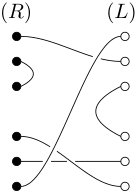 Figure 1
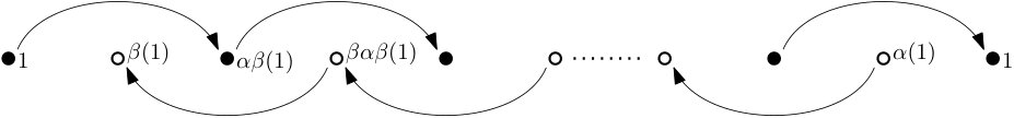 Figure 2
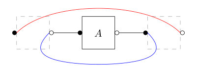 Figure 3
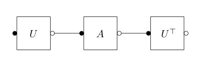 Figure 4
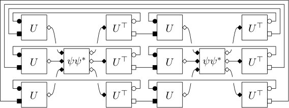 Figure 5
Peer Reviews
No public reviews on file for this paper yet. If you reviewed it on a platform where reviews are public (OpenReview, ICLR, NeurIPS, ICML), you can paste yours below so the community can read it here.
Videos
No videos yet. Explain this paper in a talk, walkthrough, or lecture? Add one.
On the minimum output entropy of
random orthogonal quantum channels
Motohisa Fukuda
MF: Yamagata University, 1-4-12 Kojirakawa, Yamagata, 990-8560 Japan
and
Ion Nechita
IN: Zentrum Mathematik, M5, Technische Universität München, Boltzmannstrasse 3, 85748 Garching, Germany and CNRS, Laboratoire de Physique Théorique, IRSAMC, Université de Toulouse, UPS, F-31062 Toulouse, France
Abstract.
We consider sequences of random quantum channels defined using the Stinespring formula with Haar-distributed random orthogonal matrices. For any fixed sequence of input states, we study the asymptotic eigenvalue distribution of the outputs through tensor powers of random channels. We show that the input states achieving minimum output entropy are tensor products of maximally entangled states (Bell states) when the tensor power is even. This phenomenon is completely different from the one for random quantum channels constructed from Haar-distributed random unitary matrices, which leads us to formulate some conjectures about the regularized minimum output entropy.
Contents
- 1 Introduction
- 2 Basics from quantum information theory
- 3 Combinatorial aspects of permutations and pairings
- 4 Invariant integration over the orthogonal group
- 5 Output states for tensor powers of random Haar-orthogonal quantum channels
- 6 Optimal sequences of input states
- 7 Discussion
1. Introduction
One of most important questions in quantum information theory is to determine the optimal rate of transmission of classical information through noisy quantum channels. Unlike its classical counterpart, no closed formula has been found yet for the classical capacity of quantum channels. Since the capacity is defined as the maximum rate at which classical information can be sent reliably over the channel in a way that the probability of error approaches zero as the length of codes goes infinity, naturally the capacity of a quantum channel has an asymptotic formula [Hol98, SW97]
[TABLE]
where is the Holevo capacity. Here, we assume that the errors appearing in the transmission of information are independent along the uses of the quantum channels , and it is represented by the tensor power in the formula.
For some classes of channels, such as depolarizing channels [Kin03a], entanglement breaking channels [Sho02, Kin03b], Hadamard channels [KMNR07], and unital qubit channels [Kin02], the above formula (1) can be simplified. This is a consequence of the following additivity property proved in the above cited papers: for any
[TABLE]
Additivity for the Holevo capacity yields a closed formula (called a single-letter formula) for the classical capacity for such channels: .
However, the above simplification does not hold for all quantum channels. In a breakthrough paper [Has09], Hastings showed violation of additivity for another quantity, the minimum output entropy, which implies that (2) does not hold for some quantum channels. These two concepts of minimum output entropy and Holevo capacity are originally different; the former only cares about single output states, while the latter deals with ensembles of outputs (see Section 2 for the exact definitions). However, previous to Hastings’ work, Shor showed [Sho04] that additivity properties for those two quantities are globally equivalent to each other, allowing the translation of counter-examples from one setting to the other.
In this paper, we focus on the minimum output entropy , which has close conceptual connection to . We inquire what kind of inputs states will minimize the output entropy for randomly chosen quantum channels. We explain briefly our methodology in three main points.
First, we choose to focus on random quantum channels. The interest in the study of random quantum channels comes mainly from the fact that, to date, violation of additivity is proved only through random techniques (typically with random unitary quantum channels generated by random unitary matrices), see [Has09, FKM10, FK10, ASW11, BCN12, Fuk14, BCN16, Col16]. Non-random counter-examples have been obtained only for -Rényi minimum output entropies, see [WH02, GHP10].
Second, our main results concern random orthogonal quantum channels. As is explained in Section 2, any quantum channel can be dilated to a unitary closed evolution on a larger space. In this work, we only consider the case where closed dynamics comes from an orthogonal rotation. The reason for this choice is that it allows us to consider identical copies of a random quantum channel, whereas if one uses the more general unitary evolutions, then one needs to take pairs of a channel and its complex conjugate to witness additivity violations:
[TABLE]
where the complex conjugation are applied to the unitary matrix which defines the channel . To translate this result into a violation inequality for two copies of the same channel
[TABLE]
one needs to restrict themselves to the real case, where the complex conjugate does not make any difference (unless one employs a particular symmetrization operation, see [FW07]).
Third, we shall fix a sequence of input states, and study the asymptotic behavior of the output states. In order to obtain the exact value of the minimum output entropy, one has to optimize over all input states for a fixed realization of the random quantum channel, but our current techniques do not allow this setting. This is indeed a drawback of our method, but in this setting we can obtain quite precise results on the possible outputs in the asymptotic limit. The current setting, where a universal, channel-independent encoding is considered, is related to the coding theory for compound quantum channels, see e.g. [DD07, BB09, Mos15].
Our main results (Theorem 6.1 and Corollary 6.2) can be informally stated as follows.
Theorem**.**
Consider random quantum channels obtained by partial-tracing the action of Haar-distributed random orthogonal matrices, where is the system dimension. Then, among fixed sequences of input states, the ones achieving minimum output entropy (asymptotically, as ) for the channels are tensor products of maximally entangled states (Bell states).
The paper is organized as follows. In Sections 2 and 3 we recall, respectively, some basics notions and facts from quantum information theory and from the combinatorial theory of permutations and pairings. In Section 4 we present the theory of invariant integration over the orthogonal group, using the graphical tensor notation. We discuss then in Section 5 the model of random quantum channels we are studying. Sections 5 and 6 are the technical core of the paper, in which we characterize the asymptotical output states for an arbitrary fixed sequence of inputs, and then we optimize over input sequences. Finally, we discuss our results and a few conjectures in the closing Section 7.
Acknowledgement. We would like to thank the referees for their very helpful comments which helped improve the quality of the presentation. I.N.’s research has been supported by a von Humboldt fellowship, the ANR project StoQ ANR-14-CE25-0003-01. M.F. was financially supported by JSPS KAKENHI Grant Number JP16K00005. I.N and M.F. are both supported by the PHC Sakura program (project number: 38615VA), implemented by the French Ministry of Foreign Affairs, the French Ministry of Higher Education and Research and the Japan Society for Promotion of Science. Both authors acknowledge the hospitality of the TU München, where this research was conducted.
2. Basics from quantum information theory
We review in this section some basic definitions and facts from quantum information theory. Some excellent references on the subject are [NC10] and [Wil17].
A quantum state is a positive semidefinite matrix with unit trace; we denote the set of quantum states by
[TABLE]
Rank one projections (here, , ) are the extremal points of the convex body of quantum states. In the case of bipartite composite systems, the state space is the tensor product . Of particular importance is the maximally entangled state , which is also called Bell state. Here,
[TABLE]
is a vector of norm (hence the normalization factor in the formula for ). We denote by the un-normalized version of . One can extend, using functional calculus, the notion of (Shannon) entropy to quantum states:
[TABLE]
a quantity which is called the von Neumann entropy of the quantum state .
Quantum channels are the most general transformations of quantum states allowed by the laws of quantum mechanics. Mathematically, quantum channels are completely positive, trace preserving maps between two matrix algebras (remember that we are concerned here only with finite-dimensional quantum systems). By the celebrated Stinespring dilation theorem [Sti55], all quantum channels can be obtained as
[TABLE]
where is an isometry, and is a parameter (called the ancilla dimension) which can be taken to be .
As explained in the introduction, quantum Shannon theory is concerned with information transmission tasks in the quantum world. One of the fundamental information processing protocols is the transmission of classical information through a noisy quantum channel. The classical capacity of a quantum channel is defined as the optimal rate (# bits transmitted) / (# uses of channel), assuming that the probability of successfully decoding the transmitted information approaches one. The mathematical theory was developed in [Hol98] and [SW97], see also [Wil17, Section 20] for a textbook presentation. The definition of the classical capacity of a given quantum channel is
[TABLE]
where is the Holevo capacity of given by
[TABLE]
where the maximum is taken over all ensembles of probability weights and input quantum states (actually, ensembles of size , where is the dimension of the input space of are enough).
The question whether the quantity is additive, i.e.
[TABLE]
is known as the additivity problem [KR01]. Shor has shown in [Sho04] that the additivity of is equivalent to the additivity of a much simpler quantity, the minimum output entropy
[TABLE]
Much of the work on the additivity problem was about the quantity , proving either that additivity holds for particular classes of channels, or providing counter-examples (see discussion and references in Section 1). The focus of the current paper is to understand, for a random orthogonal quantum channel , how additivity is violated and to find input states achieving .
3. Combinatorial aspects of permutations and pairings
As the reader shall see in the next section, the theory of invariant integration over the orthogonal group is intimately connected to the combinatorial theory of pairings and permutations. We gather in the current section the necessary definitions and basic facts from combinatorics, as well as some useful lemmas.
We denote by the symmetric group on elements. For a permutation , we denote by the number of its cycles (including fixed points). The quantity is called the length of , and it can be shown to be equal to the minimal number of transpositions that multiply to . Also, is the distance between and the identity permutation inside the Cayley graph of generated by all transpositions. Permutations satisfy triangle inequality: , and when the equality holds, we say that is on a geodesic connecting and , and express it as
[TABLE]
We write for the set of products of disjoint transpositions. The set is in bijection with the set of pairings of . To any permutation , we associate an unoriented graph , which has vertex set and edge set . It is obvious that each vertex has degree 2 (a loop at a vertex contributes degree 2 to that vertex) and that the cycles of are in bijection with the connected components of . In particular, it holds that has connected components. We investigate next a similar setting, where the permutation is replaced by a set of pairings.
To a pair of pairings of the set , encoded by permutations , we associate an unoriented graph having vertex set , and edge set given by
[TABLE]
with the convention that we allow multiple (in our case, at most 2) edges between two vertices. The following lemma is implicit in [CŚ06, Lemma 3.5]
Lemma 3.1**.**
The number of connected components of the graph is .
Proof.
First, note that for . Indeed, choose so that is non-crossing, but it implies that
[TABLE]
based on the well-known fact on non-crossing permutations [NS06].
Next, we count the number of connected components of for . To do so, we analyze the connected component which includes . Suppose a number, say, is connected to in the graph . Then, we have the following two exclusive cases.
[TABLE]
i.e. we can reach by applying and in turn because of the idempotent property: . Hence, we now have identified the connected component which includes as a disjoint union of two sets of vertices:
[TABLE]
Indeed, we have
[TABLE]
Hence, a connected component in the graph always consists of two loops generated by and for some , so that the number of connected components is . In fact,
[TABLE]
This completes the proof. ∎
To understand the proof more intuitively see Figure 1. All numbers connected to are represented by black and white dots, where from left to right for some . The left part of (8) corresponds to the black dots and the right the white dots. Note that and those arrows represent applications of .
4. Invariant integration over the orthogonal group
Since the technical core of the paper consists of moment computation for random, Haar distributed orthogonal matrices, we review in this section the Weingarten formula for averaging over the orthogonal group.
Following the work of Weingarten [Wei78], the modern mathematical formulation was developed by Collins and Śniady in [CŚ06]; some further elements can be found in [CM09, Ban10]. The orthogonal Weingarten formula provides a combinatorial expression for the average of a monomial in the entries of a Haar orthogonal matrix.
Theorem 4.1**.**
[CŚ06, Corollary 3.4]** For every choice of indices and , we have
[TABLE]
The odd moments vanish:
[TABLE]
The Weingarten function is a combinatorial function, which can either be seen as the matrix inverse of the loop counting matrix in the Brauer algebra or as a sum over Young diagrams, see [CŚ06]. The values of this function for can be found in [CŚ06, Section 6]. In [CŚ06, Theorem 3.13], the authors also compute the leading order in the large asymptotic expansion of the orthogonal Weingarten function:
[TABLE]
where is the Möbius function that we define next (see [CŚ06, Section 3.3]). Let be the number of cycles of the permutation having length (this number is indeed even, see Lemma 3.1). Then, define
[TABLE]
where is the -th Catalan number
[TABLE]
In [CN10] and [CN11], the authors introduced a graphical calculus for computing expectation values of expressions involving random unitary matrices and, respectively, random Gaussian matrices. We present next an natural extension of these ideas to integrals over the orthogonal group with respect to the Haar measure. We shall be brief in our exposition, since the procedure is very similar to the one in [CN10], also described at length in [CN16, Section III.C]. We shall encode tensors (i.e. vectors, linear forms, matrices, bipartite matrices, etc.) by boxes having labels attached to them corresponding to the respective vector spaces. Empty labels are associated to duals of vector spaces (linear forms, or “inputs” of matrices), while filled labels correspond to primal spaces (that is vectors, or “outputs” of matrices). Wires connect an empty label with a filled one of the same shape, corresponding to the same vector space. In other words, wires encode tensor contractions . Presented with a diagram (a collection of boxes and wires) containing boxes associated to a Haar distributed random orthogonal matrix , we can interpret the Weingarten formula (11) as a graph expansion corresponding to the sum over the pairings and . To each term in the sum we associate a new diagram which is obtained by deleting the boxed corresponding to the random matrix , and adding wires encoding the product of delta functions in (11). For each pair contained in , a wire is added between each primal vector space (i.e. filled label) of the boxes corresponding to the -th and the -th matrix . Similarly, wires are added between the empty labels, according to the permutation . We have thus, assuming contains -boxes,
[TABLE]
Let us showcase the formula above using a simple example. Let , and let us compute , for a Haar orthogonal matrix . Here, , so there is only one possible pairing . The original diagram and the graph expansion are represented in Figure 2. We conclude that
[TABLE]
5. Output states for tensor powers of random Haar-orthogonal quantum channels
We consider the following model of random quantum channels. We fix an integer and a real number , which are the parameters of the model. For each integer , consider the random quantum channel , where and
[TABLE]
where is a Haar distributed random isometry. Note that although is a real matrix, the matrix in (15) is an element of . The random isometry can be obtained by truncating a Haar-distributed random orthogonal matrix .
Now we investigate the sequence of random matrices, which are output states of tensor powers of random Haar-orthogonal quantum channels, with some fixed sequence of input states. More precisely, given a fixed sequence of input states , with , , let
[TABLE]
Our goal in this section will be to characterize the asymptotic behavior of the sequence of random matrices . In this setting, the parameters are fixed.
The first result is a formula for the moments of the random matrices . Let be the order of the moment and we wish to compute . We shall use the graphical orthogonal Weingarten formula from Section 4. We have depicted the diagram for , in the case , in Figure 3.
The diagram corresponding to the -th moment contains random orthogonal matrices . We shall index these matrices by a triple , where
- •
the label indicates the index of the copy of the matrix the box belongs to;
- •
the label denotes the index of the channel in the tensor power;
- •
the position label indicates whether the box appears on the “left” side of the picture or on the “right” side (i.e. the matrix appears without or with a transposition in (15)).
We introduce now two permutations which encode the initial wiring (tensor contractions) appearing in the diagram. To this end, we identify the set of integers with the set of triples described above. We put
[TABLE]
In the second equation above, we abuse notation and write for any index and position . It is important to notice that both permutations above are products of disjoint transpositions, so . As we shall see, the permutations encode the wirings corresponding to the partial trace (for each quantum channel) and, respectively, to the trace appearing in the moment of .
The graphical formulation of the Weingarten formula for integrals over the orthogonal group gives
[TABLE]
where the sum ranges over pairs of pairings of the set of boxes containing the random isometry ; the permutation is responsible for pairing the “outputs” of the boxes (corresponding to black labels), while pairs the inputs (i.e. white labels). Let compute explicitly the content of a given diagram :
- (1)
Loops corresponding to the partial traces in the quantum channel. Since the original wiring of the boxes corresponding to these loops is encoded by the permutation , the contribution of these loops is , by Lemma 3.1. 2. (2)
Loops coming from the matrix multiplication, giving a total contribution of (for the same reasons as above). 3. (3)
The contribution of the input state, let us call it for now.
Let us bound the contribution of the input state . To this end, notice that , where is a matrix encoding the pairing , having inputs corresponding to labels and outputs corresponding to labels , see Figure 4 for an example.
Let us define, for a pairing where , its number of bumps as the number of pairs inside which connect elements on the “side”. For the pairing in Figure 4, we have , since there is only one “bump” on the side. It is obvious that the number of “bumps” on the side is also , and that, up to multiplying from the left and from the right with some unitary operators, the matrix is a tensor product of unnormalized maximally entangled states with the identity operator up to rotations. In particular, we have , and thus, using Hölder’s inequality, we conclude that
[TABLE]
In order to get a better understanding of the number of bumps of a pairing, let us call a pairing transverse if it maps the side to the side and vice-versa. In other words, is transverse if for all , , and . Note that transverse pairings have zero bumps. We claim the following expression for the number of bumps of a given pairing :
Lemma 5.1**.**
For
[TABLE]
Moreover, the minimum is achieved if and only if . Here, where for each pair or supports a bump in R or L side, respectively, and where .
Proof.
To prove our claim, we can assume without loss of generality that , i.e., all elements are supporting elements of bumps, and . This is because for each transposition where and are from R and L sides, respectively, we can restrict ourselves to transverse such that in search for the minimum of .
To begin with, we prove in (19). Consider the bumps on side and name the supporting elements in pairs by where . Then, for a transverse we have the following mapping of : for
[TABLE]
for some distinctive elements from side, i.e., for . Suppose consists of disjoint cycles, say, , so that
[TABLE]
where is the cardinality of cycle . Here, we have based on the comment at the beginning of this proof. Now, each mapping in (20) constitutes a part of some cycle. If is related to mappings in (20), then . This implies that
[TABLE]
The equality holds if and only if and . In this case, the condition implies that . This complets the proof. ∎
Lemma 5.2**.**
Given elements , define two permutations in .
[TABLE]
Then, such that is of the form:
[TABLE]
for some . Here we used the notation from (5).
Proof.
We decompose
[TABLE]
and work on each component for the geodesic because and both respect this decomposition. Note that, at fixed , the only elements on the geodesic are the restrictions of and on the 4-element set:
[TABLE]
while the intermediate permutations do not belong to . The proof is now complete, since each block of must be either of type or of type. ∎
With these ingredients in hand, and with the asymptotic formula for the Weingarten function from (12), we can calculate the general term in the sum (17) and upper bound its absolute value as follows (remember our notations of and in (16)):
[TABLE]
By using (19) in Lemma 5.1 the exponent of (the only variable which grows) in the RHS of (27) reads
[TABLE]
where we have used the triangle inequality and the fact that the permutation is transverse. To identify the leading order terms in (17) we then try to ignore as many terms as possible by getting rid of terms which do not saturate the three bounds (18), (28) and (29). Note that we consider the bound (18) only asymptotically, as one can see below.
First, the equality must hold in (29). Since is a transverse, Lemma 5.1 shows that must be of the form
[TABLE]
In other words, must be a product of symmetrical bumps and horizontal wires. Here, , and is defined by a set of particular types of transpositions:
[TABLE]
Also, we abuse notations by writing to denote fixed points in by all transpositions in .
Second, the equality in (28) holds if and only if lies on the geodesic between and . This is equivalent via Lemma 5.2 to the fact that has the following form for such that and:
[TABLE]
In other words, consists of horizontal lines and a subset of the bumps of .
Third, we discuss when the equality in (18) is asymptotically saturated when . To this end, we define the number of “non-trespassing” bumps for defined in (30). For this aim, we define
[TABLE]
where “” means that the left transposition is one of transpositions constituting , so that we have the definition of .
Now, we need a lemma:
Lemma 5.3**.**
For defined in (30), we have the following bound for .
[TABLE]
Proof.
Let be a maximally entangled state associated to , i.e. a tensor product of maximally entangled states, each of which is defined by a transposition in (see Section 2 for the definitions). Then, using the general “linearization trick”
[TABLE]
we get
[TABLE]
where and are reduced density operators of in the first and second spaces, and we have used the trivial matrix inequality . ∎
This means that we can reduce candidates of leading order terms in (17), and for writing purpose we define the set of non-trespassing bumps by
[TABLE]
Note that trivially . Then, finally, we can state the result giving the asymptotic moments of the sequence of random matrices . From here on, we identify with .
Theorem 5.4**.**
*For any given sequence of input states ,
- All moments of are expressed as*
[TABLE]
where
[TABLE]
2) For the first and second moments of one can replace by .
Proof.
For pairings and as in (33), resp. (30), the Möbius function is given by (13):
[TABLE]
Also note that for in (30). Neglecting terms in (26) which vanish according to the above discussions, the general moment an be written, except for the factor, as
[TABLE]
which is the general formula we wanted. Moreover we can replace by for , based on Lemma 5.3 and the remark following it. ∎
Next, we calculate the average output state for a fixed input . To this end, we introduce a useful notation before going onto our theorem. Define for
[TABLE]
where we denote by the (un-normalized) maximally entangled state with , see also Section 2. We write for the operator acting on the copies and of the space . We also abuse notation so that means that stays fixed by transpositions in . Then,
Theorem 5.5**.**
[TABLE]
where
[TABLE]
Proof.
Now we calculate “the first moment without trace”. To this end, we just replace in (40) by . In fact where for . ∎
Theorem 5.6**.**
For a fixed sequence of input states we have the following convergence in probability:
[TABLE]
Proof.
Using the second part of Theorem 5.4, the second moment of is a sum indexed by sets . For such a , we write where these two belong to blocks with respectively, so that, using the notation from Theorem 5.4, we can factorize
[TABLE]
Then, the formula in (40) with , which represents the second moment, up to terms, changes into:
[TABLE]
where are defined by , respectively. Then, Chebyshev’s inequality shows for each
[TABLE]
This completes our proof of the convergence in probability. ∎
Remark 5.7**.**
For some models of random unitary channels, it is possible to show that similar convergence results hold almost surely, a stronger convergence that the convergence in probability proven here. This is enabled by better controlling the error in equations such as (42), up to terms. This is one technical difference between random unitary and random orthogonal matrices: in the former case, the error in the approximation of the Weingarten formula (12) is , while in the latter it is , see [CŚ06].
6. Optimal sequences of input states
Having computed in the previous section the asymptotic behavior of the outputs for a fixed sequence of input state, we turn now to the problem of finding the input sequences giving the outputs with least entropy (asymptotically). Our strategy is to show that for any sequence of input states, the outputs will lie, asymptotically, inside a fixed, deterministic set . We shall then minimize the entropy for states inside this convex set .
We start by writing the expected value of an output state into a more compact form. In what follows we replace by the set of partial parings on because in this section the parameter is more relevant. Starting from in (43), we have
[TABLE]
where the operators and for are defined as follows:
[TABLE]
where one can see the last equality via binomial formula.
Note that equation (47) is close to what we want: to express the output of the channel as a convex combination of simple quantum states. The problem here is that, although the scalars are non-negative, the matrices are not, in general, positive semidefinite. In fact, we have . In order to achieve our goal, we shall apply the Möbius inversion formula [Rot64] to (47). First, it is quite obvious to see that the Möbius function on the lattice is identical to the one for the lattice of subsets: if a partial pairing is contained in another partial pairing , then . Hence, if we define
[TABLE]
we have, via the Möbius inversion formula
[TABLE]
and we can rewrite (47) as
[TABLE]
From (48), we can actually obtain an explicit formula for the matrices :
[TABLE]
where
[TABLE]
is indeed a quantum state (i.e. a positive semidefinite matrix of unit trace); such states, convex mixtures between a maximally entangled state and a maximally mixed state are called isotropic states in the quantum information theory literature.
We have now all the ingredients to state the main result of this section.
Theorem 6.1**.**
Consider a sequence of random quantum channels constructed from random Haar distributed orthogonal matrices , as in Section 5. Furthermore, assume that for some constant and define, for any , the convex set
[TABLE]
Then, for any fixed sequence of input states , the output states converge, in probability, to the convex body : for all ,
[TABLE]
Note that depends on via (51).
Proof.
Let us fix a sequence of input states and use the triangle inequality:
[TABLE]
We have shown in Theorem 5.6 that the second term in the right hand side of the above inequality converges in probability towards zero; it is enough thus to show that the first term also vanishes as . From (49), we have the following decomposition
[TABLE]
To finish the proof, we show next that the weights in the equation above are (asymptotically) non-negative and sum up to one. For the claim about the sum, note that
[TABLE]
proving the claim. The other claim follows from [FN14, Corollary 3.6], where it was shown that the spectrum of the matrices is at distance from the set . The reader should make note of the fact that although the matrices are indexed by different combinatorial objects (partial pairings here and partial permutations in [FN14]), they encode the same linear operators and thus they have the same spectrum. ∎
Corollary 6.2**.**
Let be a maximal partial pairing in , i.e. a pairing consisting of pairs and, when is odd, a singleton. Then, for any fixed sequence of input states , the inputs
[TABLE]
give output states having less entropy than the sequence of inputs : for all ,
[TABLE]
In other words, the sequence of input states consisting of a tensor product of maximally entangled states and, when is odd, a maximally mixed state yields the output sequence with least asymptotical entropy.
Proof.
By the theorem, the outputs belong, when is large, to the set . The extremal points of are precisely the quantum states , with a partial pairing of . Such an extremal state has von Neumann entropy
[TABLE]
where is the bipartite quantum state define in (51); it has entropy strictly less than , more precisely
[TABLE]
where . To finish the proof, we show that the input sequence produces the output sequence . Indeed, from (49), we have
[TABLE]
By direct inspection, and using the fact that is a maximal partial pair pairing, we have that (see also [FN14, Section 3])
[TABLE]
and thus
[TABLE]
finishing the proof. ∎
7. Discussion
In this work, using Weingarten calculus on the orthogonal group, we have shown that among fixed input sequences for a tensor power of a random orthogonal quantum channel, product of maximally entangled states achieve the smallest output entropy. We consider our results to be evidence toward the claim that such random channels do not violate (asymptotically, with high probability) the additivity relation. More precisely, for we conjecture that, almost surely for random orthogonal quantum channels such as the ones in Section 5
[TABLE]
For this conjecture we must refer to a sentence in [Has09]: “This two-letter additivity conjecture would enable us to restrict our attention to considering input states with a bipartite entanglement structure, possibly opening the way to computing the capacity for arbitrary channels”. Hastings conjectures thus the following additivity for quantum channels:
[TABLE]
In [FN14], we have studied this question in the frame work of the current work, but with random unitary quantum channels. Then, we have shown that among a very large class of fixed input sequences, tensor products of maximally entangled states yield the outputs with least entropy. This is a strong supporting mathematical evidence towards Hastings’ conjecture. In the same direction, see [Mon13, FN15] for considerations about upper bounds on the amount of additivity violations for random quantum channels.
Surprisingly, if we compare our calculations with ones for unitary random quantum channels from [CFN12], we are inclined to conjecture that generically entanglement does not help to improve minimum output entropy of tensor powers of random unitary quantum channels, while (only) bipartite entanglement helps for random orthogonal channels: almost surely,
[TABLE]
where and are sequences of respectively unitary and orthogonal random quantum channels.
We also conjecture that similar phenomena might occur for the Holevo capacity too, and we hope that such results might shed light on capacity formulas. Indeed, according to [CFN15], certain random quantum channels satisfy a simple linear relation between their Holevo capacity and their minimum output entropy, while such a linear relation was initially observed in [Hol05] for covariant channels.
The reference list from the paper itself. Each links out to its DOI / PubMed record.
- 1[ASW 11] Guillaume Aubrun, Stanisław Szarek, and Elisabeth Werner. Hastings’ additivity counterexample via Dvoretzky’s theorem. Communications in mathematical physics , 305(1):85–97, 2011.
- 2[Ban 10] Teodor Banica. The orthogonal weingarten formula in compact form. Letters in Mathematical Physics , 91(2):105–118, 2010.
- 3[BB 09] Igor Bjelakovic and Holger Boche. Classical capacities of compound and averaged quantum channels. IEEE Transactions on Information theory , 55(7):3360–3374, 2009.
- 4[BCN 12] Serban Belinschi, Benoît Collins, and Ion Nechita. Eigenvectors and eigenvalues in a random subspace of a tensor product. Inventiones mathematicae , 190(3):647–697, 2012.
- 5[BCN 16] Serban T Belinschi, Benoit Collins, and Ion Nechita. Almost one bit violation for the additivity of the minimum output entropy. Communications in Mathematical Physics , 341(3):885–909, 2016.
- 6[CFN 12] Benoît Collins, Motohisa Fukuda, and Ion Nechita. Towards a state minimizing the output entropy of a tensor product of random quantum channels. Journal of Mathematical Physics , 53(3):032203, 2012.
- 7[CFN 15] Benoit Collins, Motohisa Fukuda, and Ion Nechita. On the convergence of output sets of quantum channels. Journal of Operator Theory , 73(2):333–360, 2015.
- 8[CM 09] Benoît Collins and Sho Matsumoto. On some properties of orthogonal weingarten functions. Journal of Mathematical Physics , 50(11):113516, 2009.