Rapid computation of $L$-functions attached to Maass forms
Andrew R. Booker, Holger Then

TL;DR
This paper introduces an efficient algorithm for computing degree-2 L-functions associated with Maass forms, enabling rapid evaluation of L-values and detailed analysis of their zeros' distribution.
Contribution
The authors develop a novel algorithm that evaluates L-functions on the critical line in near-linear time, facilitating extensive zero distribution studies.
Findings
Successfully computed many consecutive zeros of L-functions.
Observed patterns in zero distribution consistent with conjectures.
Demonstrated the algorithm's efficiency and accuracy.
Abstract
Let be a degree- -function associated to a Maass cusp form. We explore an algorithm that evaluates values of on the critical line in time . We use this algorithm to rigorously compute an abundance of consecutive zeros and investigate their distribution.
Click any figure to enlarge with its caption.
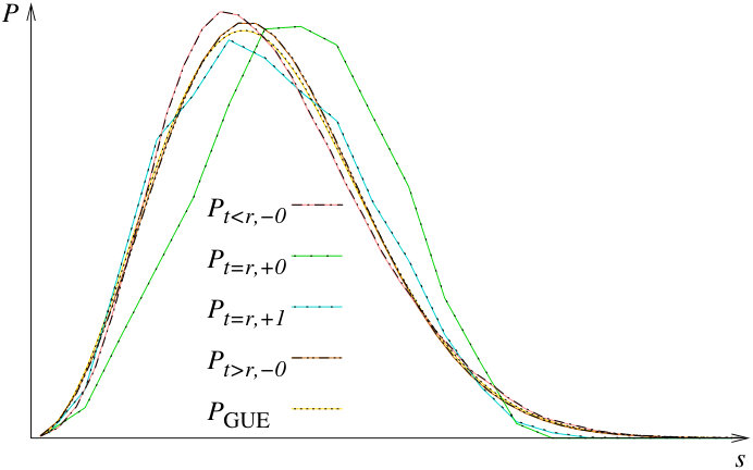 Figure 1
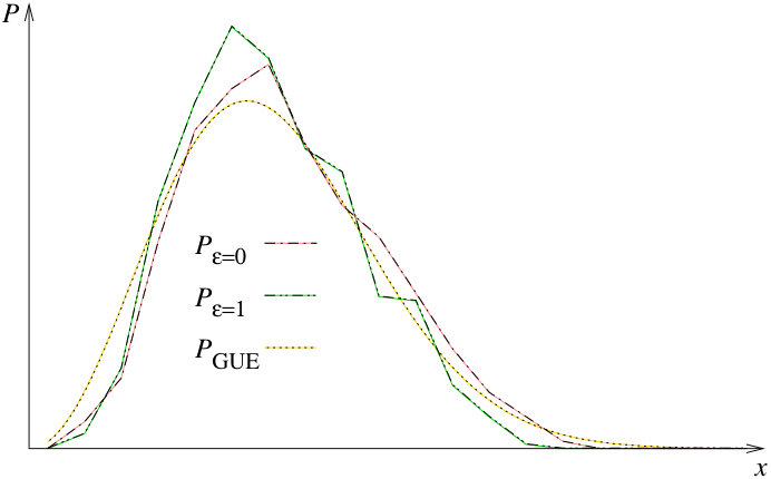 Figure 2
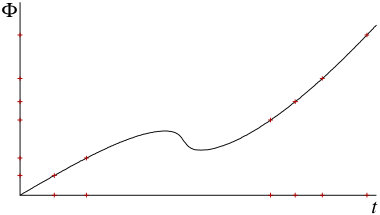 Figure 3
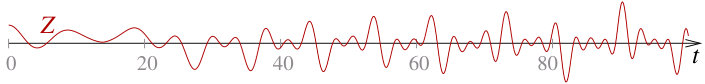 Figure 4
Peer Reviews
No public reviews on file for this paper yet. If you reviewed it on a platform where reviews are public (OpenReview, ICLR, NeurIPS, ICML), you can paste yours below so the community can read it here.
Videos
No videos yet. Explain this paper in a talk, walkthrough, or lecture? Add one.
Rapid computation of -functions attached to Maass forms
Andrew R. Booker
Department of Mathematics, University of Bristol, University Walk, Bristol, BS8 1TW, United Kingdom, e-mail: [email protected]
and
Holger Then
Alemannenweg 1, 89537 Giengen, Germany, e-mail: [email protected]
Abstract.
Let be a degree- -function associated to a Maass cusp form. We explore an algorithm that evaluates values of on the critical line in time . We use this algorithm to rigorously compute an abundance of consecutive zeros and investigate their distribution.
The authors wish to express their thanks to Andreas Strömbergsson and Pankaj Vishe for offering deep insight into their methods. H. T. thanks Brian Conrey, Dennis Hejhal, Jon Keating, Anton Mellit, and Franzesco Mezzadri for inspiring discussions. A. B. and H. T. acknowledge support from EPSRC grant EP/H005188/1.
1. Introduction
In [2], the first author presented an algorithm for the rigorous computation of -functions associated to automorphic forms. The algorithm is efficient when one desires many values of a single -function or values of many -functions with a common -factor. In this paper, we explore the prototypical case of a family of -functions to which that does not apply, namely Maass cusp forms in the eigenvalue aspect.
As described in [2, §5], one of the main challenges when computing -functions is the evaluation of the inverse Mellin transform of the associated -factor. Rubinstein [16] describes an algorithm based on continued fractions that performs well in practice, but for which it seems to be very difficult to obtain rigorous error bounds. On the other hand, the algorithm in [2], following Dokchitser [7], uses a precomputation based on simpler power series expansions that are easy to make rigorous; it works well for motivic -functions of low weight, but suffers from catastrophic precision loss when the shifts in the -factor grow large, as is the case for Maass forms.
A well-known similar problem occurs when one attempts to evaluate an -function high up in the critical strip. Rubinstein, following an idea of Lagarias and Odlyzko [12], has demonstrated that this can be dealt with effectively by multiplying by an exponential factor to compensate for the decay of the -factor; specifically, for a complete -function of degree , one works with for a suitable . This idea can be made to work for general -functions, including those associated to Maass forms (albeit with the problems related to precision loss noted above, if the -factor is not fixed), and Molin [13] has worked out rigorous numerical methods in quite wide generality.
For the specific case of Maass cusp forms, Vishe [19] (see also [8]) has shown that the “right” factor to multiply by to account for the variation in both and the -factor shifts is not the exponential function , but rather the hypergeometric function
[TABLE]
where denotes the parity of the Maass form, and is its Laplacian eigenvalue. To understand the motivation for this factor, consider first the case of a classical holomorphic cuspform , for which the -function is defined via the Mellin transform
[TABLE]
Since is holomorphic and vanishes in the cusp, we can change the contour of integration from to for some ; writing for , we obtain
[TABLE]
Thus, Rubinstein’s exponential factor arises naturally from a contour rotation.
For a Maass form of weight [math] and even parity (say), we similarly have the integral representation
[TABLE]
Since is no longer holomorphic in this case, we cannot simply rotate the contour in this expression, but we are free to start with the rotated integral and try to relate it back to . As we show in §2, this can be done, and the two are related essentially by the factor (1.1).
We analyze this strategy in greater detail in §2, but the upshot is that to compute Maass form -functions for a wide range of values of and , it suffices to compute for suitable values of and . In turn, using modularity to move each point to the fundamental domain, the problem reduces to computing the -Bessel function for various and . Fortunately, that is a problem that underlies all computational aspects of Maass cusp forms and has been well studied; see, for instance, [3].
Numerical results
In §8, using as input the rigorous numerical Maass form data of [1] we compute values of the corresponding Maass form -functions and use the resulting numerical data to test conjectures about the distribution of zeros of Maass form -functions in the - and -aspects. In particular, we show that the phenomenon of zero repulsion around that Strömbergsson observed [18] disappears in the large eigenvalue limit.
We derive rigorous error estimates and use the interval arithmetic package MPFI [15] throughout our computations to manage round-off errors. Thus, modulo bugs in the software or hardware, our numerical results are rigorous.
2. Preliminaries on Maass forms
Let be a cuspidal Maass newform and Hecke eigenform of weight [math] and level . Then has a Fourier expansion of the form
[TABLE]
where is the th Hecke eigenvalue of , is its eigenvalue for the hyperbolic Laplacian , indicates the parity, and
[TABLE]
Moreover, is related to its dual via the Fricke involution, so that
[TABLE]
for some complex number with .
Associated to we have the -function , defined for by the series
[TABLE]
It follows from (2.1) that continues to an entire function and satisfies a functional equation relating its values at and . To see this, let denote the Gauss hypergeometric function
[TABLE]
and consider the family of -factors
[TABLE]
where and is a parameter. By [9, Sec. 6.699, Eqs. 3 and 4], we have
[TABLE]
for . (Note that for a Maass form with odd reflection symmetry, viz. , (2.2) has a removable singularity at ; this is related to the fact that the complete -function is the Mellin transform of rather than .) Making the substitution , we can express the complete -function as the Mellin transform of the Maass form along a ray in the upper half plane:
[TABLE]
Splitting the integral at and employing (2.1) completes the analytic continuation:
[TABLE]
Using that and making the substitution , we obtain the functional equation:
[TABLE]
In particular, for .
3. Rigorous computation of -functions
We describe an algorithm based on the fast Fourier transform that allows one to evaluate quickly, if one is interested in many points.
The integral (2.3) is essentially a Fourier transformation,
[TABLE]
Similarly for the integral (2.2),
[TABLE]
In order to use the fast Fourier transform to compute
[TABLE]
we first need to discretize the integral. To that end, let be parameters such that is an integer. In the Poisson summation formula,
[TABLE]
we solve for , which results in
[TABLE]
[TABLE]
In §4 we will derive precise bounds for this error term.
4. Bounds
Let be the analytic conductor, defined by
[TABLE]
Note that satisfies the recurrence . Further, we define
[TABLE]
so that .
Lemma 4.1**.**
[2, §4]** For in the strip ,
[TABLE]
Remark 4.2**.**
The estimate in Lemma 4.1 is not optimal since, for for large , the right-hand side grows quadratically in , whereas the convexity estimate would give . Moreover, for and the bound becomes useless, since , whereas . Nevertheless, the estimate is clean and uniform in all parameters, and suffices for our purposes if we keep away from .
Corollary 4.3**.**
For in the strip ,
[TABLE]
with
[TABLE]
Proof.
Recall that satisfies the recurrence, reflection, and duplication formulas
[TABLE]
Hence, for and ,
[TABLE]
which yields
[TABLE]
for .
On the critical line we have
[TABLE]
and by the Phragmén-Lindelöf theorem,
[TABLE]
Thus, in the strip we have
[TABLE]
Using the Kim–Sarnak estimate [11] with in the Euler product gives
[TABLE]
Inserting the last three bounds in Lemma 4.1 yields the corollary. ∎
Lemma 4.4**.**
For with and ,
[TABLE]
with
[TABLE]
Proof.
For we have the integral representation (3.1). Since , it is enough to prove the lemma for non-negative .
Making the change of variables and moving the contour of integration back to the real line, we get
[TABLE]
and
[TABLE]
We bound the first integral using the estimates [3, p. 106] and , and the second integral using and . ∎
Lemma 4.5**.**
For with , , and ,
[TABLE]
Proof.
Using Lemma 4.4 together with yields the stated bound. ∎
Lemma 4.6**.**
For with , , and ,
[TABLE]
Proof.
By Corollary 4.3 and Lemma 4.4,
[TABLE]
Applying the estimate and summing up results in the stated bound. ∎
Lemma 4.7**.**
For , , , , and ,
[TABLE]
Proof.
Applying , , and in the Fourier expansion of the Maass form gives
[TABLE]
and by Fricke involution
[TABLE]
For ,
[TABLE]
Writing , , , with and , we have
[TABLE]
Summing the resulting geometric series gives
[TABLE]
for , and similarly for the sum over .
For ,
[TABLE]
Writing , , , with and , we have
[TABLE]
and summing up gives
[TABLE]
∎
Lemma 4.8**.**
*For , , , , and
,*
[TABLE]
Proof.
We have and , so that
[TABLE]
Writing , , , with and , we have
[TABLE]
and summing the geometric series yields
[TABLE]
for .
The argument is slightly different for the sum over . Using that [3, p. 107] and , we have
[TABLE]
for . ∎
The following two Lemmata show that we can circumvent division by zero in .
Lemma 4.9**.**
For any with , is an increasing function of .
Proof.
It suffices to show that . Suppose first that . Then, differentiating Binet’s formula for , we have
[TABLE]
For , this is easily seen to be minimum at , so we obtain
[TABLE]
For we use the reflection formula to see that
[TABLE]
and apply the above to obtain a bound for . We calculate that
[TABLE]
and with a little calculus we see that this is bounded in modulus by . Thus, altogether we have
[TABLE]
for all and . Note that the right-hand side is strictly increasing for . Using the known value , it is straightforward to see that is positive for . ∎
Lemma 4.10**.**
For , , , , and ,
[TABLE]
Proof.
We follow the proof of [17], generalizing it and making the implied constants explicit. Using [9, Sec. 9.132, Eq. 1] and writing
[TABLE]
we get
[TABLE]
By Lemma 4.9, for and ,
[TABLE]
Next,
[TABLE]
and for ,
[TABLE]
Hence for ,
[TABLE]
where stands for a value of absolute size at most .
implies that or . Thus
[TABLE]
Adjusting the phase factor in (4.3) suitably, i.e. taking and with , respectively, completes the proof. ∎
5. Interpolating zeros
We compute values of on a grid, but we are ultimately interested in the zeros, which are not regularly spaced. To zoom in on the zeros, we interpolate
[TABLE]
with and , respectively. The function has the advantage that it decays rapidly at and is approximately bandlimited, which allows us to use the Whittaker–Shannon sampling theorem [5]
[TABLE]
Truncating the sum over and bounding the error of truncation, we get an effective interpolation formula for .
Lemma 5.1**.**
For , , , and ,
[TABLE]
Proof.
For , we have , and for , we bound by (4.1). Hence,
[TABLE]
∎
Lemma 5.2**.**
For , , , and ,
[TABLE]
Proof.
The proof is similar to that of the previous lemma, except that for we bound by Lemma 4.4. ∎
Lemma 5.3**.**
For , , , , and ,
[TABLE]
Proof.
By Fourier convolution,
[TABLE]
with , as defined in (2.3a). Using (4.2) and writing gives
[TABLE]
Changing the order of integration, we have
[TABLE]
Let and set . For , we have and , while for , . Moreover, for , , ,
[TABLE]
while for ,
[TABLE]
Thus,
[TABLE]
Identifying the integrals with the complementary error function and the incomplete gamma function completes the proof. ∎
Lemma 5.4**.**
For , , , , and ,
[TABLE]
Proof.
By Fourier convolution,
[TABLE]
with , as in (2.2a). For , we have [3, p. 107], , and . Hence, writing , we have
[TABLE]
For , we use , and to obtain
[TABLE]
Therefore, after interchanging the order of integration,
[TABLE]
where we have employed for , and otherwise. Evaluating the integrals completes the proof. ∎
6. Detecting zeros
For each Maass form -function under consideration, we compute rigorously many values on the critical line. For instance, Figure 1 shows a graph of
[TABLE]
for the first even Maass form -function on .
Corollary 6.1**.**
Let be the set of zeros on the critical line of the -factor. For values of and chosen according to Lemma 4.10,
[TABLE]
Proof.
This follows immediately from Lemma 4.10. ∎
Remark 6.2**.**
Fixing the value of , say , there is a risk of hitting a zero of (to within the internal precision) when evaluating for some specific value of . In all of our computations, we never observed this in practice, i.e. we never had to deal with division by zero. However, computing at finite absolute precision, we sometimes come close to a zero of and experience some loss of precision in the division by . Since we also compute for a second value of , , chosen according to Lemma 4.10, we may always ensure the accuracy of the computed values of .
For each Maass form -function under consideration, we rigorously compute all zeros on the critical line up to some height. The search for zeros is faciliated by the following lemma.
Lemma 6.3**.**
(a) Let be real valued, and assume it has consecutive simple zeros at , and , with . Then such that the following holds:
[TABLE]
(b) Let be real valued, and assume it has a zero of order at , with . Then such that the following holds:
[TABLE]
for , but .
Proof.
The lemma follows from elementary analysis and the intermediate value theorem. ∎
Algorithm 6.4**.**
Let be real valued. Let be a strictly increasing sequence of real numbers. Refine the sequence until all zeros of are isolated, i.e. there is at most one zero per interval .
Remark 6.5**.**
If the quadrants of for consecutive are not ordered as given in Lemma 6.3(a), there is either a zero of order greater than which is to be investigated according to Lemma 6.3(b), or the sequence is not yet fine enough. We expect the sequence to be fine enough if for successive the quadrants of do change by at most by , and when they change, they do so in agreement with Lemma 6.3.
There is no proof that the expectation in Remark 6.5 holds, and one can construct sequences that contradict the expectation. Nevertheless, with some reasonable choices in the construction of the sequence and its refinements, the expectation turns out to be reliable in practice. Namely, for every Maass form -function that we considered, we never overlooked any zero, as proven after the fact using Turing’s method.
7. Turing’s method
Turing’s method for verifying the Riemann hypothesis for arbitrary -functions is described in [2]. For not the ordinate of some zero or pole of , let
[TABLE]
By convention, we make upper semicontinuous, i.e. when is the ordinate of a zero or pole, we define .
We select a particular branch of by using the principal branch of . With this choice, set
[TABLE]
We further define
[TABLE]
which relates to the number of zeros in the critical strip up to height . For let denote the multiset of zeros with imaginary part in , and let denote their number, counting multiplicity,
[TABLE]
Then, we have
[TABLE]
Theorem 7.1**.**
[2, §4]** For and , define
[TABLE]
and
[TABLE]
Suppose and satisfy
[TABLE]
for some , and set
[TABLE]
Then
[TABLE]
Corollary 7.2**.**
For , assume is a given multiset of zeros with imaginary part in , i.e. . Let
[TABLE]
If
[TABLE]
exceeds the right-hand side of the bound in Theorem 7.1, then the set contains all zeros with imaginary part in . .
Proof.
If were a proper subset of , then we would have , whence . But the integral of the latter is bounded by Theorem 7.1. ∎
8. Numerical results
We consider consecutive Maass cusp forms on . Booker, Strömbergsson, and Venkatesh [4] have rigorously computed the first Maass cusp forms on to high precision. Bian [1] has extended these computations to a larger number of Maass cusp forms. The readily available list of rigorously computed Maass cusp forms is consecutive for the first Maass cusp forms, which covers all Maass cusp forms whose Laplacian eigenvalue falls into the range .
Previous numerical computations of some non-trivial zeros for a few even Maass form -functions were made by Strömbergsson [18]. We extend his results by rigorously computing, for each of the first consecutive Maass form -functions on , many values of , including all non-trivial zeros up to , at least.
Remark 8.1**.**
At the time of Strömbergsson’s work, even the numerical data pertaining to the Maass cusp forms for was not rigorously proven to be accurate, so he had no reason to carry out his computations of the zeros with more than heuristic estimates for the error. Making use of the rigorous data sets described above, we have rigorously verified the correctness of Strömbergsson’s results. In particular his lists of zeros are consecutive and accurate. Moreover, we confirm his observation of a zero-free region on the critical line for near , when is small.
We note that some theoretical results, such as Cho’s theorem [6] on simple zero of Maass form -functions, assumed the correctness of Strömbergsson’s numerical results. With our verification, Cho’s theorem becomes unconditional.
Our lists of zeros contain more than consecutive non-trivial zeros per Maass form -function. All these zeros are simple. The first several zeros of the first five Maass form -functions are listed in Table 1.
Theorem 8.2**.**
For a Maass cusp form on with spectral parameter , all non-trivial zeros with of the corresponding Maass form -function are simple and on the critical line.
Proof.
For each Maass form -function we prove, using Corollary 7.2, that the corresponding list of rigorously computed zeros is consecutive for , and that all the zeros are indeed simple and on the critical line. ∎
According to a conjecture of Montgomery [14], the distribution of non-trivial zeros should follow random matrix theory (RMT) predictions. In case of Maass form -functions, the distribution of non-trivial zeros is expected to conform to that of eigenvalues of large random matrices from the Gaussian unitary ensemble (GUE) [10]. This raises the question of how GUE statistics relate to the zero-free region around observed by Strömbergsson [18]—are the GUE statistics asymptotically correct in the large aspect only?
We investigate this question by distinguishing between zeros with small and large absolute ordinate, respectively. For a given Maass form -function there are only a finite number of zeros with small ordinate, and the resulting statistics would be poor. Knowing the zeros for many Maass form -functions, we can evaluate on a common scale the distribution of zeros for each -function and collate the statistics of many of them together.
Let be a Maass cusp form with spectral parameter and parity . Consider the zeros of the associated Maass form -function. We unfold the zeros,
[TABLE]
in order to obtain rescaled zeros with a unit mean density. Then defines the sequence of nearest-neighbor spacings, which has mean value as . Now, the distribution of nearest-neighbor spacings is given by
[TABLE]
where the index denotes the corresponding Maass cusp form. Distributions of rescaled nearest-neighbor spacings are expected to be independent of the specific parameter values of corresponding Maass cusp forms and can be collated by writing
[TABLE]
To distinguish between zeros with small and large absolute ordinate, we define the respective nearest-neighbor spacings distributions,
[TABLE]
where is a non-negative integer, as well as their collated versions
[TABLE]
For the first Maass form -functions on , the resulting distributions are displayed in Figure 2, in comparison with the Wigner surmise
[TABLE]
As is visible, the distribution of zeros resembles GUE statistics for both small and large absolute ordinate, and there appears to be no distinction between the statistics of the two cases. Only the distribution of zeros that are in absolute size closest to the value of the spectral parameter might show a stronger level repulsion than the Wigner surmize.
However, it is unclear whether this seemingly stronger level repulsion is just an artefact of the limited number of spacings that contribute to the histogram of . If we take three times as many spacings into account, as is the case with , we again find a close resemblance to the Poisson distribution. We speculate that the GUE statistics hold for all , not only in the large aspect.
Since the GUE statistics are based on rescaled zeros, , they do not contradict a zero-free region on the critical line. The density of zeros is described by , and according to the -factor, the density of zeros is smaller for in a neighborhood of . In particular, for small values of the spectral parameter , the density becomes negative for near ; see Figure 3. There are finitely many Maass form -functions on that have such a region where is negative. By inspection, we find that no zero falls into a negative density region. Moreover, the zeros seem to be repelled away from the negative density regions resulting in the zero-free region around .
Finally, we investigate the repulsion from zero of the rescaled first zero in dependence of the parity of the Maass form -function. For this we consider the distributions of the rescaled first zero,
[TABLE]
for . The resulting distributions are displayed in Figure 4. Close to the origin of the plots, they show a stronger level repulsion than the Wigner surmise .
The reference list from the paper itself. Each links out to its DOI / PubMed record.
- 1[1] C. Bian, A. R. Booker, and M. Jacobson, Unconditional computation of the class groups of real quadratic fields, in preparation.
- 2[2] A. R. Booker, Artin’s conjecture, Turing’s method, and the Riemann hypothesis, Experiment. Math. 15 (2006), 385–408.
- 3[3] A. R. Booker, A. Strömbergsson, and H. Then, Bounds and algorithms for the K-Bessel function of imaginary order, LMS J. Comp. Math. 16 (2013), 78–108.
- 4[4] A. R. Booker, A. Strömbergsson, and A. Venkatesh, Effective computation of Maass cusp forms, Int. Math. Res. Notices 2006 (2006), article ID 71281.
- 5[5] J. L. Brown Jr., On the error in reconstructing a non-bandlimited function by means of the bandpass sampling theorem, J. Math. Anal. Appl. 18 (1967), 75–84.
- 6[6] P. J. Cho, Simple zeros of Maass L 𝐿 L -functions, Int. J. Number Theory 9 (2013), 167–178.
- 7[7] T. Dokchitser, Computing special values of motivic L 𝐿 L -functions, Experiment. Math. 13 (2004), 137–149.
- 8[8] A. Good, On various means involving the Fourier coefficients of cusp forms, Math. Z. 183 (1983), 95–129.