Numerical homogenization of elliptic PDEs with similar coefficients
Fredrik Hellman, Axel M{\aa}lqvist

TL;DR
This paper introduces a parallelizable Petrov-Galerkin localized orthogonal decomposition algorithm for efficiently solving sequences of elliptic PDEs with similar, rapidly varying coefficients, applicable in time-dependent and stochastic contexts.
Contribution
The paper develops an adaptive PG-LOD method that selectively recomputes local correctors, improving efficiency for sequences of similar elliptic PDEs.
Findings
The method effectively handles sequences with similar coefficients.
Adaptive recomputation enhances computational efficiency.
Application demonstrated on 3D time-dependent Darcy flow.
Abstract
We consider a sequence of elliptic partial differential equations (PDEs) with different but similar rapidly varying coefficients. Such sequences appear, for example, in splitting schemes for time-dependent problems (with one coefficient per time step) and in sample based stochastic integration of outputs from an elliptic PDE (with one coefficient per sample member). We propose a parallelizable algorithm based on Petrov-Galerkin localized orthogonal decomposition (PG-LOD) that adaptively (using computable and theoretically derived error indicators) recomputes the local corrector problems only where it improves accuracy. The method is illustrated in detail by an example of a time-dependent two-pase Darcy flow problem in three dimensions.
Click any figure to enlarge with its caption.
 Figure 1
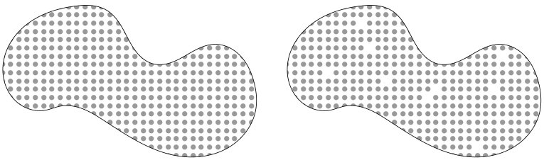 Figure 2
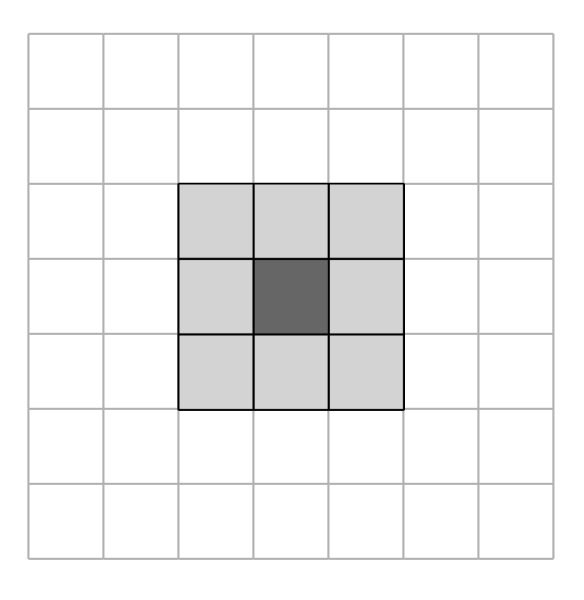 Figure 3
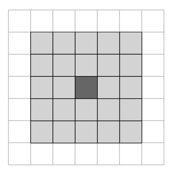 Figure 4
 Figure 5
 Figure 6
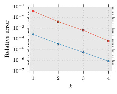 Figure 7
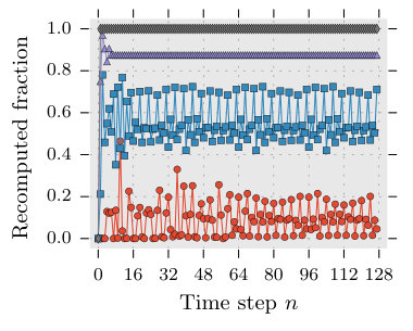 Figure 8
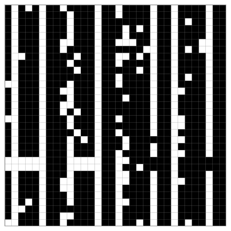 Figure 9
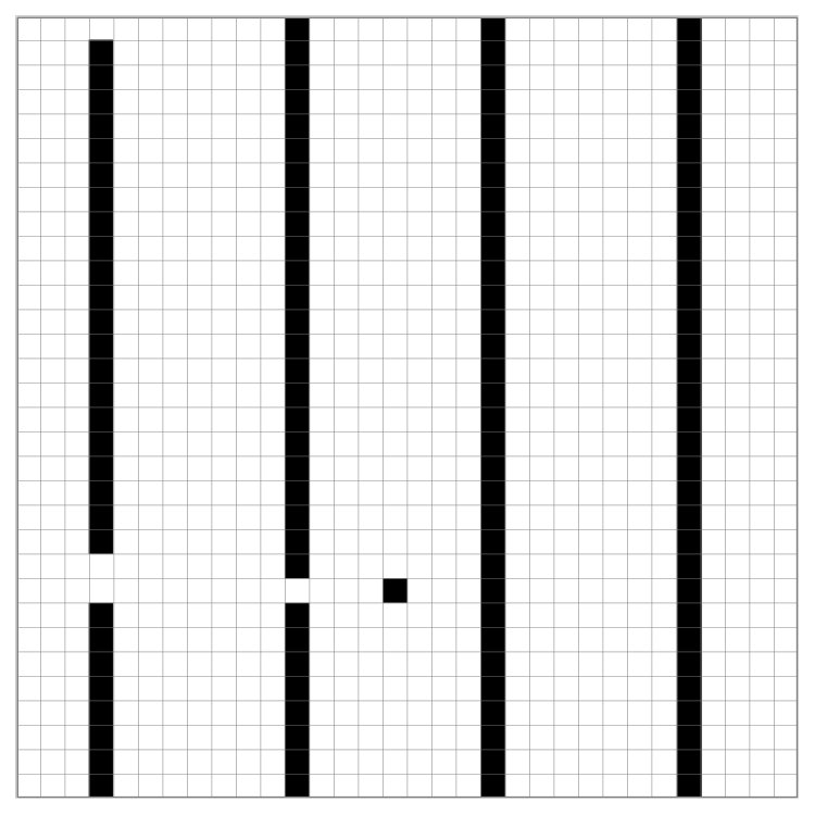 Figure 10
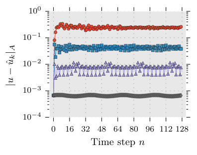 Figure 11
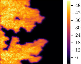 Figure 12
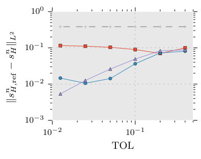 Figure 13
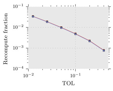 Figure 14
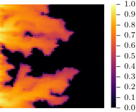 Figure 15
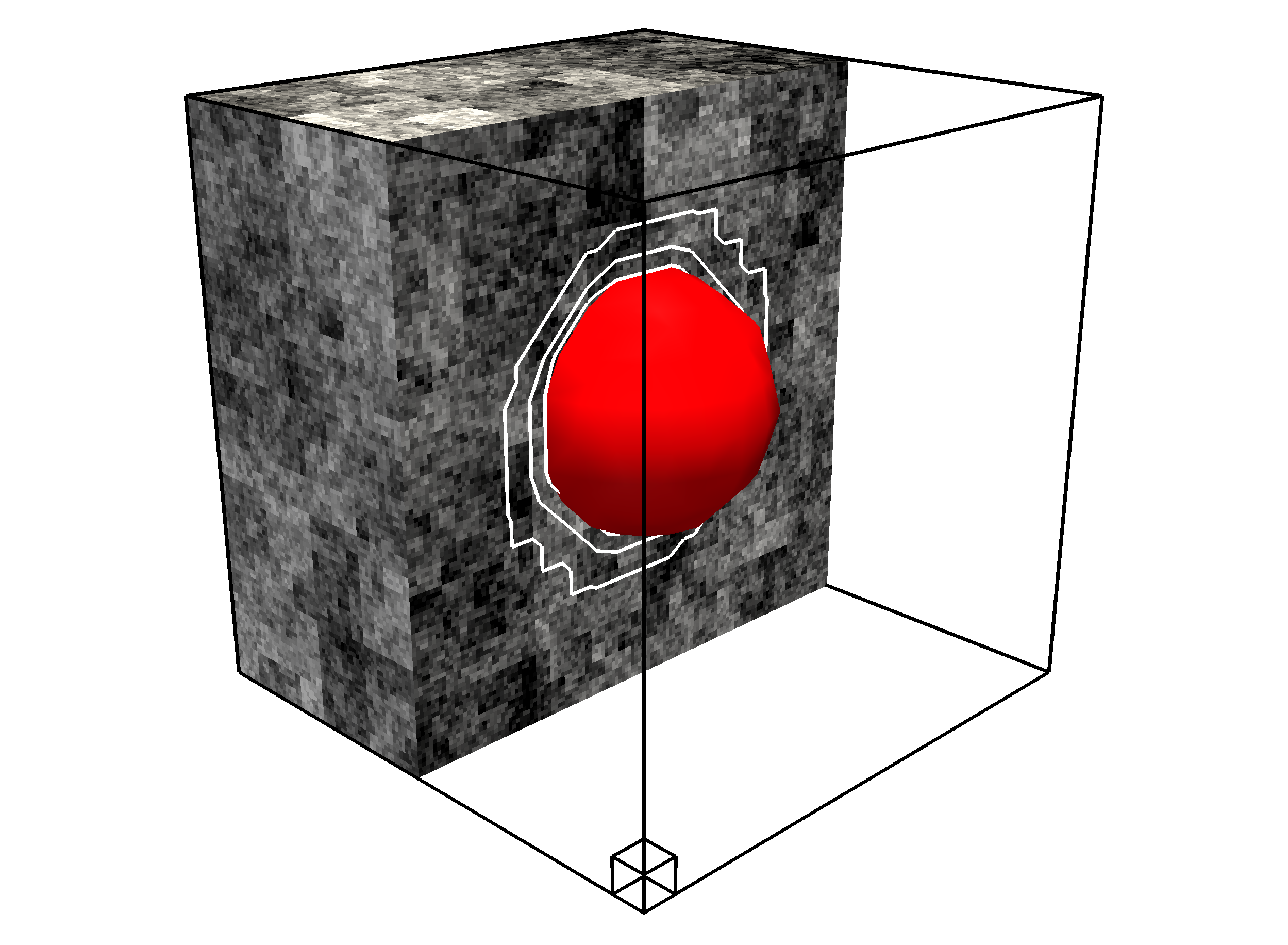 Figure 16
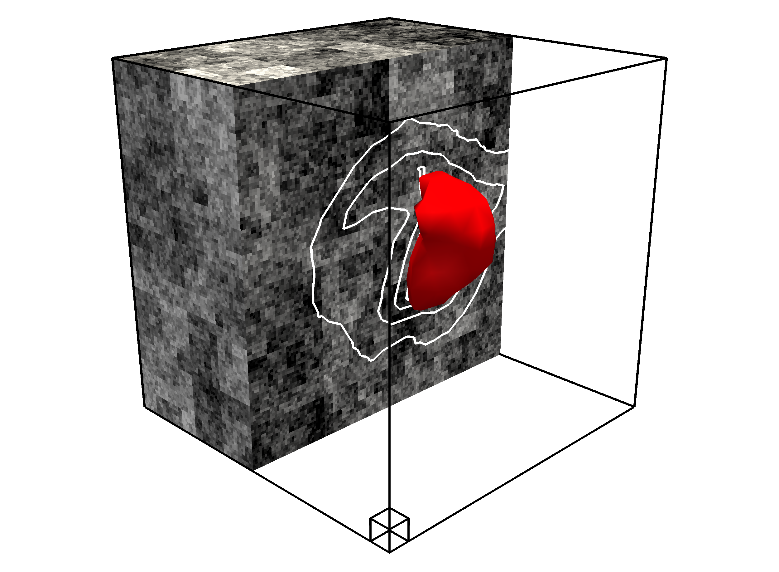 Figure 17
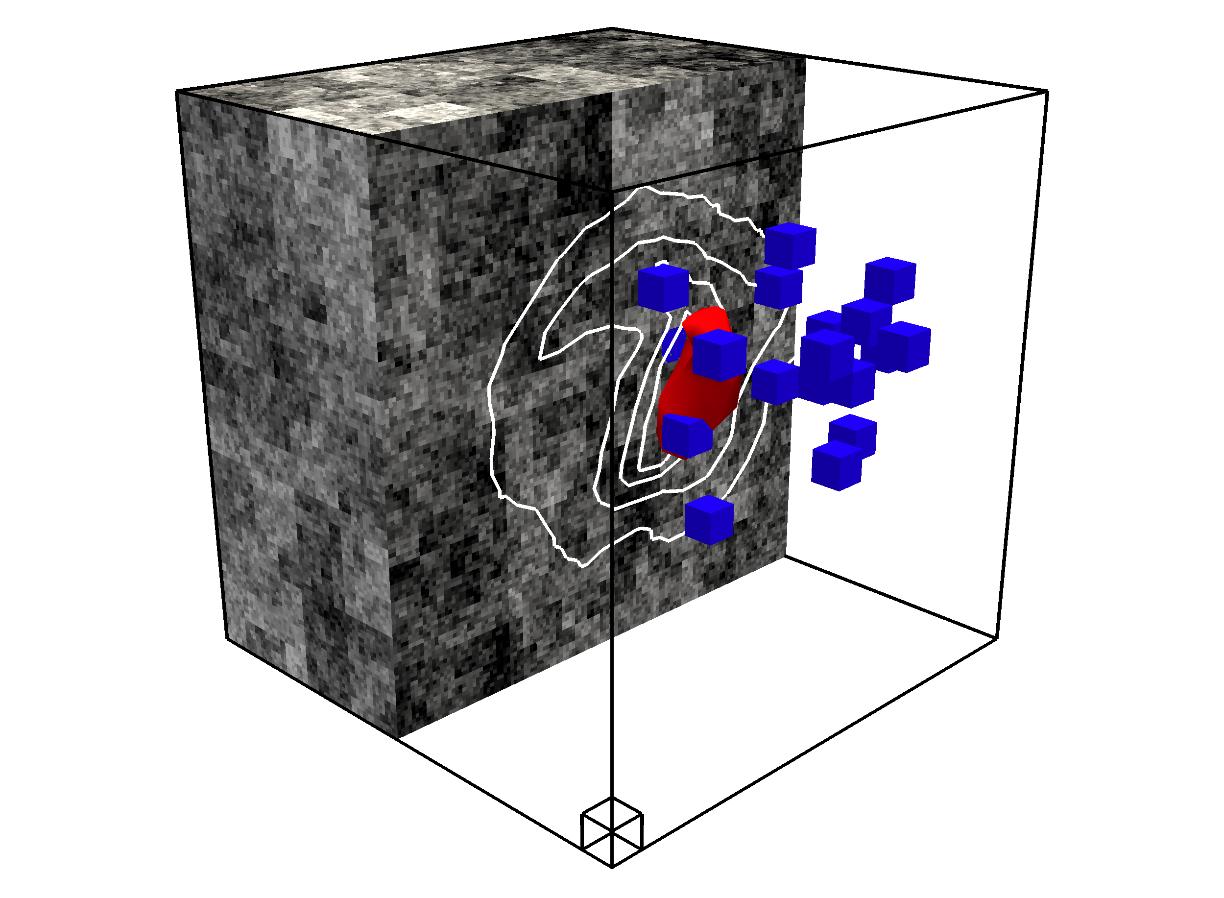 Figure 18
Peer Reviews
No public reviews on file for this paper yet. If you reviewed it on a platform where reviews are public (OpenReview, ICLR, NeurIPS, ICML), you can paste yours below so the community can read it here.
Videos
No videos yet. Explain this paper in a talk, walkthrough, or lecture? Add one.
Taxonomy
TopicsAdvanced Mathematical Modeling in Engineering · Advanced Numerical Methods in Computational Mathematics · Composite Material Mechanics
Numerical homogenization of elliptic PDEs with similar coefficients
Fredrik Hellman Department of Information Technology, Uppsala University, Box 337, SE-751 05 Uppsala, Sweden. Supported by Centre for Interdisciplinary Mathematics (CIM), Uppsala University.
Axel Målqvist Department of Mathematical Sciences, Chalmers University of Technology and University of Gothenburg SE-412 96 Göteborg, Sweden. Supported by the Swedish Research Council.
Abstract
We consider a sequence of elliptic partial differential equations (PDEs) with different but similar rapidly varying coefficients. Such sequences appear, for example, in splitting schemes for time-dependent problems (with one coefficient per time step) and in sample based stochastic integration of outputs from an elliptic PDE (with one coefficient per sample member). We propose a parallelizable algorithm based on Petrov–Galerkin localized orthogonal decomposition (PG-LOD) that adaptively (using computable and theoretically derived error indicators) recomputes the local corrector problems only where it improves accuracy. The method is illustrated in detail by an example of a time-dependent two-pase Darcy flow problem in three dimensions.
1 Introduction
We consider a sequence of elliptic partial differential equations (PDEs) with different, but in some sense similar, rapidly varying coefficients. In some applications, the difference between consecutive coefficients in the sequence is localized, for example for certain Darcy flow applications and in the simulation of random defects in composite materials. This paper studies an opportunity to exploit that the differences are localized to save computational work in the context of the localized orthogonal decomposition method (LOD, [20]).
The accuracy of Galerkin projection onto standard finite element spaces generally suffers from variations in the coefficient that are not resolved by the finite element mesh. The work [3] studies an elliptic equation in 1D with a rapidly varying coefficient and notes that coefficient variations within the element lead to inaccurate solutions for the standard finite element method. Replacing the coefficient with its elementwise harmonic average leads to an accurate method. This result, however, does not easily generalize to higher dimensions. For periodic and semi-periodic coefficients varying on an asymptotically fine scale, a homogenized coefficient can be computed and used for coarse scale computations also in higher dimensions [5]. The early multiscale method [15] is based on homogenization theory and works under assumptions on scale separation and periodicity. Many recent contributions within the field of numerical homogenization can be used without assumptions on periodicity and in higher dimensions, see e.g. [4, 16, 18, 20, 23]. In this work, we consider the LOD technique [20] in the Petrov–Galerkin formulation (PG-LOD) studied in detail in [9].
The fundamental idea of the LOD method is that a low-dimensional function space (multiscale space) with good approximation properties is constructed by computing localized fine-scale correctors to the basis functions of a standard low-dimensional coarse finite element space based on a coarse mesh. Each localized corrector problem is posed only within a patch of a certain radius around its coarse basis function and thus depends only on the diffusion coefficient in that patch. The PG-LOD method has several good properties from a computational perspective. The main advantage is that the PG-LOD corrector problems can be computed completely in parallel with the only communication being a final reduction to form a low-dimensional global stiffness matrix. Further, the fine-scale coefficient only needs to be accessible and stored in memory for one localized corrector problem at a time. Additionally, the method is robust in the sense that both the localized corrector problems and the global low-dimensional problems are typically small enough to be solved with a direct solver.
Once computed, the correctors can be reused for problems with the same or similar diffusion coefficient. We study the case when the diffusion coefficient varies in a sequence of problems. In such situations, there is an opportunity to reuse previously computed localized correctors if the coefficients do not vary too much between consecutive problems. Since the computational cost is proportional to the number of localized corrector problems that have to be recomputed, it is most advantageous if the perturbations of the coefficient are localized. Two practical examples are two-phase flow where the coefficient depends on the saturation of the two fluids, or when the coefficient is a deviation from a base coefficient as in the case with defects in composite materials.
In this work we derive computable error indicators for the error introduced by refraining from recomputing a corrector after a perturbation in the coefficient. The method we propose computes all localized correctors and global stiffness matrix contributions for the first coefficient in the sequence of elliptic PDEs. For the subsequent coefficients, we use the error indicators to adaptively recompute only the correctors that need to be recomputed in order to get a sufficiently accurate solution. The coefficients that have not been recomputed we call lagging coefficients. The method is completely parallelizable over the elements of the coarse mesh. A particularly interesting setting is when only quantities on the coarse mesh are required from the solution, for example upscaled Darcy fluxes in a Darcy flow problem, or the coarse interpolation of the full solution. Any computed fine scale quantities can then be forgotten between the iterations in the sequence and the memory requirement becomes very low.
The paper is divided into five sections: Problem formulation in Section 2, method description in Section 3, error analysis in Section 4, implementation in Section 5, and numerical experiments in Section 6. Both the method description and the error analysis are divided into four steps, with increasing level of approximation in each step: (i) reformulation by variational multiscale method (VMS), (ii) localization by LOD, (iii) approximation of localized correctors by lagging coefficient, and (iv) approximation of global stiffness matrix contribution by lagging coefficient. The main results are the method (12) in Section 3.4, the error bound in Theorem 4 and Algorithm 1.
2 Problem formulation
Let be a polygonal domain in (with or ) with the boundary partitioned into disjoint subsets (for Dirichlet boundary conditions) and (for Neumann boundary conditions). Suppose we have a sequence of elliptic equations: for , solve for , such that
[TABLE]
where , , is the outward normal of the boundary, and is a coefficient varying significantly over small distances. To keep the presentation short, we limit ourselves to the case where and are independent of , however, the analysis in this paper can be generalized to -dependent and . We will refer to the sequence index or rank as time step throughout the paper, although it does not need to correspond to a step from a time-disceratization. For instance, in Section 5 we briefly discuss an application for simulation of weakly random defects in composite materials, where the sequence index corresponds to a Monte Carlo sample member index.
In the remainder of this section and Sections 3–4, we consider a fixed step and drop this index for all quantities. We call the coefficient at the current time step the true coefficient. Ideally, only the true coefficient would be used in the solution at the current time step. However, in order to lower the computational cost, computations from previous time steps will be reused. This means coefficients from previous time steps (lagging coefficients) will enter the analysis through the definition of the localized correctors and in the assembly of the global stiffness matrix. These lagging coefficients will be denoted by . We also want to emphasize that the error indicators derived here are applicable also to situations where the coefficient deviates from a base coefficient, for example within the application of simulations of weakly random defects in composite materials.
We will work with a weak formulation of the above problem. Let . In case is empty, we instead consider only solutions and test functions in the quotient space . Let denote the -scalar product over , and . Further, we define , , and the bilinear form . We let , where and is an extension of the boundary condition to the full domain and seek to find , such that for all ,
[TABLE]
Assuming there exist constants and , so that a.e., is bounded and coercive on and existence of a unique solution is guaranteed by the Lax–Milgram theorem. We further define the energy norm on , and the semi-norm .
3 Method description
In this section, we describe the proposed numerical method in a series of steps, each of which introduces another level of approximation for the problem (2) above.
3.1 Variational multiscale method
The first step is to reformulate the problem using the variational multiscale method [16, 17]. This formulation forms the basis for the LOD approximation and makes it possible to reduce the dimensionality of the problem once the corrector problems have been solved.
Let be a regular and quasi-uniform family of conforming subdivisions of into elements of maximum diameter , and be a family of conforming first order finite element spaces on this mesh, e.g. or depending on the shape of the elements. The choice of a linear projective quasi-interpolation operator defines the fine space as its kernel . We assume there exists a constant independent of so that for all and , it holds
[TABLE]
Here is the union of all neighboring elements to , i.e.
[TABLE]
Since we assume is projective (this is not strictly necessary, see e.g. [9]), we have the decomposition and can decompose the solution and test function and test (2) with the two spaces separately:
[TABLE]
We note that is linear in and , and we define the linear correction operators and , so that , i.e., find and , such that for all ,
[TABLE]
These equations have unique solutions, since is still bounded and coercive on a subspace .
We introduce a new space, the multiscale space, , and note that we have the orthogonality relation . The solutions , , and can be plugged into (4a) and we get the following low-dimensional Petrov–Galerkin problem, find , such that for all ,
[TABLE]
The full solution is then .
Remark 1** (Right hand side correction ).**
It is possible to obtain an approximate solution even if neglecting the right hand side correction term, i.e. letting above. See for example [14, 20].
3.2 Localized orthogonal decomposition
The second step is to localize the corrector computations by means of localized orthogonal decomposition (LOD). The basic idea is to solve the corrector problems (5) only on localized patches instead of on the full domain to reduce the computational cost.
For the localization, we define element patches for , , where . With trivial case , (a -layer element patch around ) is defined by the recursive relation
[TABLE]
See Figure 1 for an illustration of element patches.
We further define localized fine spaces
[TABLE]
consisting of fine functions which are zero outside element patches. Throughout the paper, localized quantities are subscripted with the patch size .
Instead of solving (5), we compute the operators and , with and defined by
[TABLE]
for all and all .
We define the localized multiscale space . Our localized multiscale problem reads find , such that for all ,
[TABLE]
and the full solution for the second approximation is .
3.3 Lagging multiscale space
In the third approximation we compute the localized element correctors using a lagging coefficient rather than the true . This makes it possible to reuse correctors that have been computed at earlier time steps, so that localized correctors only for a small number of elements need to be recomputed.
We define the lagging localized corrector operators and . The element corrector operators are defined such that for all ,
[TABLE]
Note that lagging coefficients are not necessarily the same for all .
Example 1** (Relation between lagging coefficient and time steps).**
As an example, for the current time step , for element the coefficient can be one time step old, i.e. and for three time steps old, i.e. . That is, different lagging localized element correctors may be defined in terms of coefficients from different time steps in history.
In analogy with previous multiscale spaces, we define a lagging multiscale space and the problem is then to find , such that for all ,
[TABLE]
and the full solution for the third approximation is .
3.4 Lagging global stiffness matrix contribution
The fourth approximation involves not only using a lagging multiscale space, but also a lagging coefficient in the assembly of the global stiffness matrix and right hand side. The rationale behind this is that computing the integrals in the stiffness matrix and right hand side for (9) requires that all precomputed element correctors are stored. To circumvent this, we propose the following approximation. First we define a lagging bilinear form (and its elementwise contributor ), based on the same lagging coefficients as was used for the multiscale space in the previous section,
[TABLE]
where is the indicator function for subset . We also define a lagging linear functional (and its elementwise contributor ),
[TABLE]
Then the problem is posed as to find , such that for all ,
[TABLE]
The full solution for the final approximation step is then .
We note that (12) coincides with (9) when for all . Also, we note that the coefficients for the linear system can be computed immediately after and have been computed. This means no correctors need to exist simultaneously.
This method is independent of the true coefficient , if not for any . In order to construct a numerical method with control of the error from this approximation, we use error indicators on the element correctors to determine whether they need to be recomputed or not. Next, we define three computable error indicators, , and , for the error introduced by using a lagging coefficient.
3.5 Error indicators
As can be seen in later Sections 4.3 and 4.4, the differences for , , and constitute the sources to the error in the approximation from using lagging coefficients. In this section, we define three elementwise error indicators (, , and ) and relate them to the above differences in Lemma 2.
Lemma 2** (Error indicators: definitions and bounds).**
The following bounds hold,
[TABLE]
where
[TABLE]
We additionally define
[TABLE]
Proof.
For any , let , then using (7) and (8), we get
[TABLE]
Then, clearly (if it exists) constitute the asserted bound. The following inequality gives a bound for the norm being maximized in the definition of (assuming that ),
[TABLE]
The maximum is thus attained and exists by the extreme value theorem.
Similarly, for , we have
[TABLE]
which motivates the definition of and the asserted bound. The result for holds analogously. ∎
Regarding the computation of these error indicators, both and are straight-forward to compute, being a ratio of two computable norms. The error indicator is also easy to compute. It is the square root of a Rayleigh quotient for a generalized eigenvalue problem (where the restriction removes the singularity of the denominator matrix):
[TABLE]
with the matrices
[TABLE]
for all where is the number of basis functions in (i.e. one of them removed). The squared maximum corresponds to the maximum eigenvalue . We emphasize that the matrices and are very small: the same size as the number of degrees of freedom in the coarse element (minus one for removing the constant), e.g., for 2D simplicial meshes or for 3D hexahedral meshes.
3.5.1 Coarse error indicators
In order to compute the error indicators , , and we need access to the true coefficient and lagging correctors , , and at the same time. This implies all lagging correctors need to be saved in order to compute the error indicators. Since the correctors in practice are defined on patches of a fine mesh, and the patch overlap can be substantial, the memory requirements for saving them might be large. In this section, we construct an additional bound that makes it possible to discard the lagging correctors after they have been computed.
We construct the following bound starting from the definition of in Lemma 2,
[TABLE]
where , and we used that
[TABLE]
in the last inequality. We further define .
The maximum in (13) corresponds to a maximum eigenvalue of a low-dimensional generalized eigenvalue problem, as was the case for in Section 3.5. More specifically, it is the square root of the maximum eigenvalue
[TABLE]
of with the matrices
[TABLE]
for , where is the number of basis functions in . We note that the quantity can be computed directly after corrector has been computed for the basis functions in element . Now, does not need to be saved for computing later, and it can be discarded. In particular, the memory required for storing (which, however, is needed to compute ) scales like .
Still, needs to be available to compute and . This might not be a problem in applications where there is a low-dimensional description of the coefficient, for example if the coefficient is defined by a set of geometric shapes which can be described by location, size, shape and so on. In the section for numerical experiments, we will study an example of upscaled two-phase Darcy flow, where we illustrate a way to avoid saving .
The error indicator can replace in all results and algorithms in this work. Similar coarse error indicators can be derived for and .
4 Error analysis
In this section we study the approximation error of the three approximations , and , and the inf-sup stability for the systems yielding the solutions , , and . Finally, in Theorem 4 in Section 4.4, we present a bound on the error of the full approximation.
We use to denote a constant that is independent of the regularity of , patch size and coarse mesh size . It can, however, depend on the contrast . The value of the constant is not tracked between steps in inequalities. By the notation , we mean .
4.1 Variational multiscale method
Since the varitional multiscale formulation (6) is only a reformulation of the original problem, without any approximations, there is no error. However, the well-posedness of the formulation is still of interest.
4.1.1 Stability
Uniqueness of a solution to (6) is guaranteed by an inf-sup condition for on and ,
[TABLE]
The existence inf-sup condition holds analogously. We let denote the inf-sup stability constant and note that it is depends on the contrast for general . See [12, 24] for corrector localization results independent of the contrast.
4.2 Localized orthogonal decomposition
For the error analysis of LOD we recite previous exponential decay results (first presented in [20]) of the localized corrector operators by means of the following lemmas. For example, the proof in [14, Lemma 3.6] is almost directly applicable here.
Lemma 3** (Localization error).**
Let be a fixed integer and let be the solution of
[TABLE]
for all , where such that for all . Furthermore, we let be the solution of
[TABLE]
for all . Then there exists a constant that depends on the contrast but not on or the variations of , such that
[TABLE]
This lemma can be applied for the localization error of both and . In analogy with the definition of as a sum of , we can define with . Then for any , we can identify with and with in the lemma above (and similarly for ).
4.2.1 Stability
Using Lemma 3, we get the following result for , with ,
[TABLE]
If in addtion , we can use the stability of and continue to get
[TABLE]
Using the result above, we can derive an inf-sup constant for and the pair of spaces and ,
[TABLE]
For sufficiently large , there is a uniform bound . See [9] for more details on stability of this approximation.
4.2.2 Error
For arbitrary , using the equations (6) and (7), we have for all ,
[TABLE]
The inf-sup condition for uniqueness above yields the following approximation result, for arbitrary ,
[TABLE]
In analogy with (15) we get the following result for ,
[TABLE]
Recall that and . Now, if we choose , then and using the approximation result we get
[TABLE]
Then, using , interpolation stability (3) and stability of the continuous problem, we have for the full error
[TABLE]
This result was first shown in [20] and is noteworthy, since the error of the approximation decays exponentially with increasing , independently of the regularity of the solution .
4.3 Lagging multiscale space
For this step, we use a lagging multiscale space and need to establish an inf-sup stability constant for with respect to and . We will use the results from Lemma 2 both for deriving stability and the approximation error. The following full corrector error can be derived using Lemma 2,
[TABLE]
The bounds and hold similarly.
We note that if , then . Obviously, updating a lagging coefficient for an element corrector leads to no error for this element corrector.
4.3.1 Stability
We can now derive an inf-sup constant for on and , using similar techniques as in (16),
[TABLE]
We note that enters the constant, but that it can be compensated by a small . Since is computable, a rule to recompute all element correctors with for some small enough , will (after recomputation) make and . This makes . Following this adaptive rule makes it possible to find a lower bound for sufficiently large and sufficiently small .
4.3.2 Error
Again, we get an approximation result from the inf-sup stability. In complete analogy with (LABEL:eq:through_interpolation) and (18), we get
[TABLE]
4.4 Lagging global stiffness matrix contribution
In the fourth approximation (12), the coefficients for the integration of the global stiffness matrix and (parts of) the right hand side are also lagging.
4.4.1 Stability
We derive an inf-sup constant for (see (10)) with respect to and ,
[TABLE]
Again, enters, but can be compensated by a small according to the discussion in Section 4.3.1. Thus, there is a bound for all sufficiently large .
4.4.2 Error
To study the error , we first note that , since the right hand side and boundary condition corrections are the same in both cases. We form the following difference from (9) and (12),
[TABLE]
Add and subtract and use Lemma 2 to get
[TABLE]
Inf-sup stability for and finally gives, for any ,
[TABLE]
We conclude this section by presenting the main theoretical result of this paper. It gives a bound of the full error of (in energy norm) in terms of the patch size and the error indicators , , and defined in Lemma 2. This theorem forms the basis for the implementation of a method that updates the multiscale space adaptively while iterating through the sequence of coefficients.
Theorem 4** (Error bound for multiscale method with lagging coefficient).**
Assume is sufficiently large, so that holds. Let and (by recomputation of element correctors) . Choose sufficiently small so that , and . Further, let solve (2) and solve (12). Let . Then
[TABLE]
where the hidden constant depends on the contrast but is independent of mesh size , patch size and regularity of the solution .
Proof.
The estimate of the full error is obtained by combining (18), (LABEL:eq:error_falsespace), and (22), and using the triangle inequality,
[TABLE]
and finally using the assumed bounds of , and . ∎
Remark 5** (Selecting parameters , and ).**
The coarse mesh size parameter is typically chosen based the desired accuracy of the computation. The localization parameter is chosen to be proportional to guaranteeing a perturbation of the approximation of the order . Finally, is chosen proportional to . The resulting error bound in energy norm then reads .
5 Implementation
In this section, we present an algorithm for computing approximate solutions to a sequence of problems as described by (1). In a practical implementation we can not let be an infinite dimensional space. We will assume that there is a finite element space based on a mesh that resolves the coefficient, which if used to solve (2), yields an approximate solution with satisfactory small error . The analysis in the previous sections holds also if replacing with , however, the error estimates will then of course be bounding instead of . In the end of the section we discuss the memory requirements of the algorithm.
The key idea is that, as time progresses, we do not update the full multiscale space, but only the parts where it is necessary for a sufficiently small error. If only changes slightly between two consecutive , it is possible that many of the element correctors (, and ) based on lagging coefficients do not need to be recomputed. We use the error indicators , and to determine for which elements to recompute correctors. This results in an algorithm that is completely parallelizable over , except for the solution of the low-dimensional (posed in ) global system. Even the assembly of the global stiffness matrix and right hand side can be done in parallel, as it becomes a reduction over .
The algorithm is presented in Algorithm 1. We denote by , the finite element basis functions spanning .
Note that the if-statement in this algorithm together with properly chosen and , ensures that the conditions for Theorem 4 are fulfilled. The numerical experiment in Section 6.1 investigates the relations between the error and and the fraction of recomputed element correctors.
The memory required to perform the main algorithm grows with in the following manner. Suppose is the number of elements in the fine discretizations, as is the case for quasi-uniform meshes. To compute , and , we need to keep , , , and between the iterations in Algorithm 1 (see Lemma 2). Since the patches overlap by coarse elements, the amount of memory required between the iterations scales like . In high dimensions for very fine meshes, the amount of memory needed for storage can become a limitation. Depending on the application, it is possible to reduce the memory requirements. Below we give two examples of such applications.
Example 2** (Defects in composite materials).**
For simulations on weakly random materials [2], we consider the coefficient of a reference material and a material with random defects shown in Figure 2. If each ball in this material has a certain low probability to be missing (a localized point defect), the proposed method can be used to solve the model problem with the defect material on the right (true coefficient) using correctors precomputed on the reference material on the left (lagging coefficient). In sample based methods for stochastic integration (e.g. Monte Carlo), the proposed method for determining what correctors to recompute can reduce the computational cost for the full simulation.
The lagging coefficient in this example is the single reference coefficient and thus the same for all and all . Because of this, no additional memory is required to store lagging coefficients in this case. If we additionally use the (less efficient) coarse error indicators , , and presented in Section 3.5.1, our memory requirement scales with between the iterations in the algorithm.
Example 3** (Two-phase Darcy flow).**
In a discretization of a two-phase Darcy flow system of equations (pressure and saturation equation) for an injection scenario, the permeability coefficient varies over time indirectly through the dependence on the saturation . Typically, the change in saturation between time steps is localized to the front of the plume of the injected fluid. Thus, most corrector problems can be expected to be reused between iterations. An approach to reducing the memory requirements for the solution of this problem is revisited in detail in Section 6.2.
6 Numerical experiments
In all numerical experiments, we use Lagrange finite elements in 2D or 3D on rectangular or rectangular cuboid elements. The degrees of freedom are the values of the polynomial in the corners of the element.
We define the interpolation operator to be used throughout the experiments. Let denote the polynomials of no partial degree greater than , i.e. for all independent variables if . We define the broken finite element space,
[TABLE]
We denote by the -projection onto and by the boundary condition conforming node averaging operator (Oswald interpolation operator), for all nodes in ,
[TABLE]
where and is the cardinality. Then we define . This operator satisfies (3), see e.g. [8].
6.1 Experiments studying the effects of and
We let , , , , , and as shown in Figure 4(a). was constructed by taking a uniform grid with cells, and assigning each grid cell a value , where was drawn from a uniform distribution between , for each cell independently. Then, the values in cells whose midpoint satisfied were set to . Finally, the values in cells whose midpoint satisfied were set to .
The space is discretized on a finite element space on a uniform grid of size , see Figure 3. The is chosen as a finite element space on the coarse mesh shown in the same figure.
6.1.1 Error decay with
First, we let and solve for for and . We solve for on the fine mesh and use that as reference solution. The exponential convergence in terms of can be observed in Figure 5.
6.1.2 Error decay with
Now we fix and define a sequence of coefficients for ,
[TABLE]
This describes a perturbation of a factor up to over the full domain, sweeping from the left to the right. We emphasize that the difference is nonzero everywhere, which means a strategy to determine which correctors to recompute is necessary. We use Algorithm 1 to compute the approximate solution for every time step . A reference solution is also computed. We do this for four values of , and .
The (relative) error in energy norm versus the time step is plotted to the left in Figure 6. The right plot in the same figure shows the fraction of all element correctors that were recomputed in each time step. We note that the error decreases with decreasing as expected and that the fraction of recomputed element correctors increase with decreasing . Without an adaptive strategy, all element correctors would have to be recomputed in every time step. See Figure 7 for two maps over the recomputed element correctors in time step for two different values of .
6.2 Low-memory Darcy flow upscaling algorithm
In order to continue with two additional numerical experiments (in Section 6.3), we describe an algorithm for pressure solution upscaling for Darcy flows that reduces the space complexity to (from ). This is done by solving the saturation equation on the coarse mesh and the pressure equation with saturation dependent diffusion coefficient on a fine mesh using the proposed adaptive multiscale method. This is possible in a situation where the diffusion coefficient cannot be averaged on the coarse mesh, but the saturation solution can. The low space complexity and the possibility to parallelize the corrector computations enable the solution of large-scale problems of this kind.
6.2.1 A Two-phase Darcy flow model problem
We consider the immiscible non-capillary two-phase Darcy flow problem using the fractional flow formulation [13, 21]. This leads to a system of a coupled pressure and saturation equation
[TABLE]
where space-time functions: , and are pressure, saturation for the wetting phase, and sources/sinks, respectively; space function is intrinsic permeability; and nonlinear scalar functions: and are total mobility and wetting phase mobility, respectively. A common technique used for solving this system is sequential splitting, where the pressure equation and saturation equation are solved separately within a time step . This means that, as we iterate in time, we need to solve a sequence of pressure equations with coefficient . Since the wetting saturation changes only significantly along the plume front between time steps, we are in the setting where consecutive differences in the coefficient is localized.
The permeability varies on a fine scale, requring these variations to be resolved by a fine mesh with mesh size in order to obtain an accurate pressure solution. We consider the case when the saturation equation needs only be solved on a coarser mesh with mesh size to obtain a sufficiently accurate saturation solution. We let the fine mesh be a refinement of the coarse mesh . The pressure and saturation equations are solved sequentially: Given initial data for the saturation, the pressure equation is solved. An approximation of the coarse element face flux is computed and used to solve for the next saturation using a zeroth order upwind discontinuous Galerkin method with explicit Euler forward time-stepping.
We use the same discretization scheme as in [22]. Let be the space of piecewise constants on the elements of . Let denote set of faces of . Each face has a normal direction (outward pointing for boundary faces). We define the jump operator over face as , where and are the outward pointing face normals of the two elements and adjacent to . Let denote the -scalar product when is -dimensional. We let the flow be completely driven by boundary conditions, i.e. . We use the following discretization for the saturation equation. Given , , find such that for all ,
[TABLE]
Here is an upscaled total flux quantity approximating (over face ) ; the sets , , and contain interior faces, Dirichlet boundary faces with outgoing and ingoing flux, respectively; is the saturation boundary condition; and is the upwind saturation
[TABLE]
where and are adjacent to and points from to ; and the function is the so called fractional flow function. The discretization of the pressure equation is: find , so that for all ,
[TABLE]
where . As suggested in [22], we define the non-conservative pre-flux be a harmonic average of the (discontinuous) element face flux at the faces. Then we use the post-processing technique presented in the same paper (with non-weighted minimization) to post-process and obtain the conservative flux used in the saturation equation.
We make two observations on the information exchange between the two equations when using this discretization:
In the pressure equation, we are only interested in the coarse scale saturation from the saturation equation. 2. 2.
In the saturation equation, we are only interested in the upscaled flux from the pressure equation.
6.2.2 Coarse error indicators
The first observation allows us to compute , and from Section 3.5.1, without saving . Suppose that for element , the lagging coefficient is from time step , and . We note that is a coarse quantity, since fine-scale cancels,
[TABLE]
Thus, to compute in (13), only for need to be saved from previous time steps. The memory required to store behaves like . Also, can be used to compute in (13).
To summarize, no lagging fine scale information needs to be stored. Only the coarse quantities and need to be saved between iterations.
6.2.3 Coarse face flux
The second observation is that we only need the coarse element face flux for the saturation equation. Since this quantity is defined on the coarse mesh, we precompute
[TABLE]
for all , for all faces and all basis functions with support in . Here, we used the harmonic average , where and are the two elements adjacent to , if is an interior face, and , where is adjacent to , if is a boundary face. The memory required for storing and scales with , since the two quantities are zero for all pairs except when .
If we now let the coarse component of the multiscale solution be expressed as , then we can compute the upscaled non-conservative face flux by
[TABLE]
The final conservative face flux is then computed using the post-processing technique developed in [22].
We conclude this section by listing the upscaling algorithm (Algorithm 2) for this two-phase Darcy flow problem. In this algorithm, the memory requirements are (where is for the coefficient which can be distributed on different computational nodes). This allows for very refined fine meshes. Also, the coarse element loop is still completely parallel, and this algorithm serves as a good candidate for a scalable memory efficient upscaling algorithm.
6.3 Darcy flow upscaling numerical experiments
In the following two experiments, we investigate the properties of the upscaling algorithm presented in the previous section. We pick the following mobility functions , , and .
6.3.1 2D random field data
We let , , , , . We use a rectangular grid as fine mesh for and a grid as coarse mesh for . The permeability is realized as a piecewise constant function on the fine mesh from a lognormal distribution with exponential spatial correlation and standard deviation , i.e. for a fine element midpoint ,
[TABLE]
where and covariance between points are
[TABLE]
with correlation length and where denotes Euclidian norm. The initial saturation is set to , and boundary conditions are set to on the left boundary, which is the only boundary with ingoing flux. The number of time steps and their size are set to and , respectively.
The upscaling algorithm was run with this setup with and , 0.2, 0.1, 0.05, 0.025, and 0.0125. A reference solution , where the pressure equation was solved on the fine mesh using the standard finite element method in every iteration was computed. To illustrate the need for upscaling, we also computed the pressure equation on the coarse mesh using the standard finite elements. See Figure 8 for plots over the error in the saturaton solution at the final time step and average fraction of recomputed correctors. In the error plot we can see that both parameters and affect the error in the chosen regimes. We note from the recomputation plot that there is no dependency between the fraction of recomputed element correctors and patch size . Figure 9 shows an example of the saturation solution and the number of times correctors have been computed.
6.3.2 3D random field data
We let , , , , . We use a rectangular grid as fine mesh for and a grid as coarse mesh for . We use a sample of independent uniformly distributed random numbers between [math] and . The permeability is a piecewise constant function on the fine uniform mesh and is defined by
[TABLE]
where are the fine element midpoints, and denotes the ceiling function. See Figure 10 for the particular realization used. The boundary conditions are set to on the boundary with ingoing flux, and the initial saturation is set to a piecewise constant function on the coarse mesh with the following values in the coarse element midpoints ,
[TABLE]
The number of time steps are set to and the time step to .
The upscaling algorithm was run for the three parameter combinations I: , , II: , , and III: , . Figure 10 gives an illustration of the solution at and . One of the images shows the recomputed elements as blue boxes and we can see that many elements are not recomputed. In this case, we were not able to compute a reference solution using the available computational resources, but we can estimate the sensitivity of the solutions with respect to the parameters and . Let , , and denote the saturation solutions at time step for the parameter combinations I, II, and III, respectively. We get
[TABLE]
These numbers suggest that the error due to localization (controlled by the parameter ) dominates in this case.
7 Conclusion
Elliptic equations with similar rapidly varying coefficients occur for instance in time-dependent problems for two-phase Darcy flow and in stochastic simulations on defect composite materials. We consider a sequence of elliptic equations, each with different coefficients , . We define a method that computes and updates an LOD multiscale space as we iterate through the coefficients. This is done by the computation of localized element correctors that depend on the coefficient in the vicinity of the element. These computations can be performed completely in parallell. We derive error indicators , , and that indicate whether or not to update the corrector at element while iterating the sequence of coefficients. By selecting a small enough tolerance for the error indicators, the multiscale space will keep its approximation properties through the sequence of coefficients. It is shown analytically and numerically that the error indicators bound the error in energy norm of the solution. We present a memory efficient upscaling algorithm for a particular application of two-phase Darcy flows.
The reference list from the paper itself. Each links out to its DOI / PubMed record.
- 1[1] R. E. Alcouffe, A. Brandt, J. E. Dendy, Jr, and J. W. Painter. The multi-grid method for the diffusion equation with strongly discontinuous coefficients. SIAM J. Sci. Stat. Comput. , 2(4):430–454, 1981.
- 2[2] A. Anantharaman and C. L. Bris. A numerical approach related to defect-type theories for some weakly random problems in homogenization. Multiscale Model. Simul. , 9(2):513–544, 2011.
- 3[3] I. Babuška and J. E. Osborn. Generalized finite element methods: Their performance and their relation to mixed methods. SIAM J. Numer. Anal. , 20(3):510–536, 1983.
- 4[4] M. Bebendorf. Low-rank approximation of elliptic boundary value problems with high-contrast coefficients. SIAM J. Numer. Anal. , 48(2):932–949, 2016.
- 5[5] A. Bensoussan, J. L. Lion, and G. Papanicolaou. Asymptotic Analysis for Periodic Structure , volume 5 of Studies in Mathematics and Its Applications . North-Holland, Amsterdam, 1978.
- 6[6] J. H. Bramble, J. E. Pasciak, J. Wang, and J. X. Convergence estimates for multigrid algorithms without regularity assumptions. Math. Comp. , 57(195):23–45, 1991.
- 7[7] Z. Chen, G. Huan, and B. Li. An improved IMPES method for two-phase flow in porous media. Transp. Porous Media , 54(3):361–376, 2004.
- 8[8] D. A. Di Pietro and A. Ern. Mathematical Aspects of Discontinuous Galerkin Methods . Springer-Verlag Berlin Heidelberg, 2012. Mathématiques et Applications, Vol. 69.