Estimating parameter uncertainty in binding-energy models by the frequency-domain bootstrap
G.F. Bertsch, Derek Bingham
TL;DR
This paper introduces the frequency-domain bootstrap (FDB) as a fast, correlation-aware method for estimating parameter uncertainties in nuclear binding-energy models, improving upon traditional techniques.
Contribution
The paper presents the FDB method for uncertainty estimation, accounting for error correlations, and demonstrates its effectiveness on nuclear binding energy models.
Findings
FDB provides more conservative uncertainty estimates.
FDB aligns better with empirical estimates.
Method is computationally efficient.
Abstract
We propose using the frequency-domain bootstrap (FDB) to estimate errors of modeling parameters when the modeling error is itself a major source of uncertainty. Unlike the usual bootstrap or the simple analysis, the FDB can take into account correlations between errors. It is also very fast compared to the the Gaussian process Bayesian estimate as often implemented for computer model calibration. The method is illustrated drop model of nuclear binding energies. We find that the FDB gives a more conservative estimate of the uncertainty in liquid drop parameters in better accord with more empirical estimates. For the nuclear physics application, there no apparent obstacle to apply the method to the more accurate and detailed models based on density-functional theory.
Click any figure to enlarge with its caption.
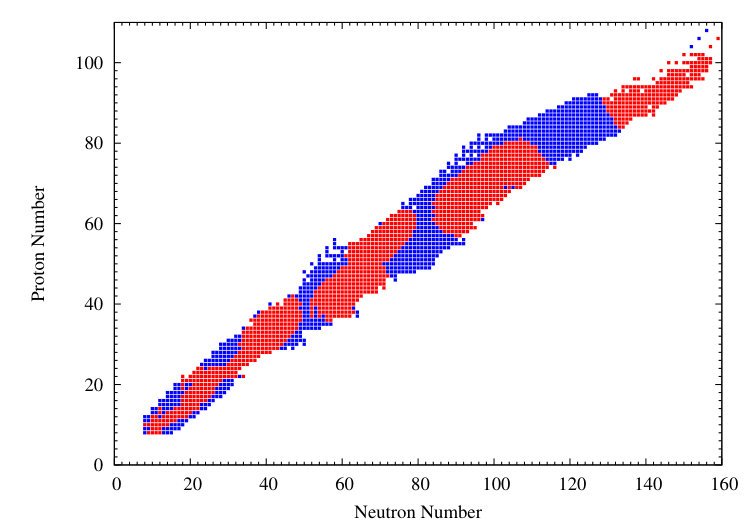 Figure 1
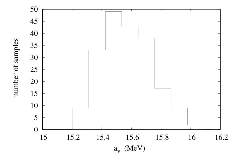 Figure 2
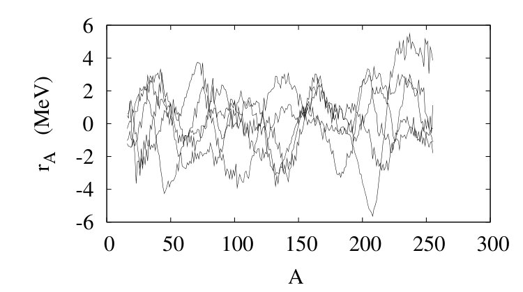 Figure 3
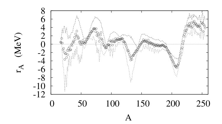 Figure 4
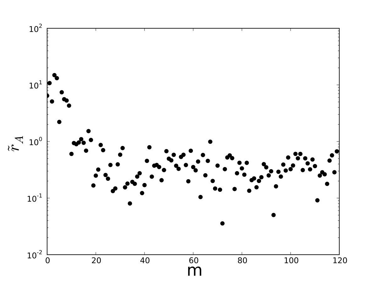 Figure 5
Peer Reviews
No public reviews on file for this paper yet. If you reviewed it on a platform where reviews are public (OpenReview, ICLR, NeurIPS, ICML), you can paste yours below so the community can read it here.
Videos
No videos yet. Explain this paper in a talk, walkthrough, or lecture? Add one.
Estimating parameter uncertainty in binding-energy models by the
frequency-domain bootstrap.
G.F. Bertsch1 and Derek Bingham2
1Department of Physics and Institute of Nuclear Theory, Box 351560
University of Washington, Seattle, Washington 98915, USA
2Department of Statistics, Simon Fraser University, Vancouver, CA
Abstract
We propose using the frequency-domain bootstrap (FDB) to estimate errors of modeling parameters when the modeling error is itself a major source of uncertainty. Unlike the usual bootstrap or the simple analysis, the FDB can take into account correlations between errors. It is also very fast compared to the the Gaussian process Bayesian estimate as often implemented for computer model calibration. The method is illustrated with a simple example, the liquid drop model of nuclear binding energies. We find that the FDB gives a more conservative estimate of the uncertainty in liquid drop parameters in better accord with more empirical estimates. For the nuclear physics application, there no apparent obstacle to apply the method to the more accurate and detailed models based on density-functional theory.
Introduction. The bootstrap method is widely used to estimate sampling distributions of statistics ef77 . We will show here that the frequency-domain bootstrap (FDB) for time series analysis (kr12, , Sect. 6) is well suited for estimating uncertainty in the modeling parameters arising in the theory of nuclear binding energies. Parameters such as the binding energy of nuclear matter and symmetry energy of nuclear matter are needed to construct models of the nuclear equation of state, which is an essential ingredient in the physics of neutron stars. We first describe the method in general terms, and then apply it to the very simple liquid-drop model of nuclear binding energies. The same approach can be applied to more sophisticated models, such those based on density-functional theory re16 , which should provide even narrower limits than can be obtained from the liquid drop description.
* and the basic bootstrap.* Estimating parameters in models and their respective uncertainties is fraught with difficulty. Obviously, if there is theoretical guidance on the functional form of the systematic difference between the system response and the model, it should be incorporated into the parameter estimation. Absent any guidance, the estimation can on be based on the model’s performance; parameters that make the model “look” like data are preferred.
Denote the model function ; it depends on parameters and maps input data variables (which may be vectors) onto output . For the nuclear physics model treated below, the variables are , the proton and neutron numbers, and is the binding energy of the nucleus.
The first step in applying a model is to determine a best-fit parameter vector, , by minimizing the square of the residual differences between the model prediction and the experimental data, . Denote the corresponding vector of the best-fit residuals by . The experimental data for this sort of procedure is implicitly specified as
[TABLE]
where is a correction or error term. The perfect model would have the form , where are the true parameters and .
Now comes the main assumption of the method: The correction terms, , are independent for each () and follow a mean zero Gaussian distribution with equal variances (the equal variance assumption specifies that the experiments have the same uncertainty and is not strictly necessary). The likelihood for the parameters is then
[TABLE]
where is the residual variance.
Broadly speaking, the bootstrap is an approach to estimating the sampling distribution of a statistic that requires few assumptions on the process that generated the data. The basic idea is that the data, or some function of the data, is repeatedly sampled with replacement. For each bootstrap sample, parameters of interest are estimated, and the ensemble of parameter estimates is the corresponding bootstrap distribution. The basic bootstrap in our setting can now be defined as an approximation to sampling distribution of the estimator of without specifying a particular error distribution. To do so, we (i) draw samples, with replacement, of residuals from the entries in the vector and (ii) reestimate . Doing this many times gives the bootstrap distribution of values. From this bootstrap distribution, functionals such as uncertainty estimates or confidence intervals can be computed.
Dealing with correlations. The , or basic bootstrap method for that matter, greatly underestimates the uncertainty of the parameter distribution in many circumstances. The reason is that the assumed ensemble has no correlation between the residuals at different points; an unlikely occurrence because if the model overestimates the system mean response at a given , it is also likely to overestimate the mean at nearby ’s as well. If the residuals are correlated, that needs to be taken into account in constructing the sampling distribution function for the estimator of , otherwise the variance in the derived sampling distribution will be too small.
Correlations can be taken into account by a Gaussian process ensemble of residuals ke01 and this method has become an accepted tool in nuclear physics mc15 ; hi15 ; pr15 ; be16 and elsewhere in physics recent under the heading of computer model calibration. This amounts to an attempt to consider any systematic signal in the residuals, as a function of , that is not accounted for by the model. The specification a Gaussian process requires that a mean function (usually taken to be a constant) and a correlation function must be chosen.
The specification in (1) is essentially the same as adopted in ke01 where their correction term is the sum of a discrepancy function and experimental error. In the applications we consider, the experimental error is a negligible component of and can be safely ignored. Therefore, is analogous to their discrepancy function. The frequency-domain bootstrap that we advocate here is an alternative way to include correlations. Furthermore, it is computationally much more efficient to the Gaussian process approaches in ke01 ; hi15 .
The Frequency-Domain Bootstrap. As before, we start with a parameter fit producing a residual vector . We need to have a measure of distance between data points, , and we assume for the moment that is one-dimensional array of contiguous integers. This allows us to define the discrete Fourier transform of the residual vector . For a residual vector of dimension , the discrete Fourier transform (and its inverse) may be expressed
[TABLE]
with in the range . The Fourier transform can also be expressed with pure real variables as
[TABLE]
If there are strong correlations of short range in , the magnitudes of the residuals will be enhanced for . On the other hand, if there are no correlations between difference points we expect the components of to be Gaussian distributed with a variance independent of . We have no information about the phases, , and we assume that they are uniformly distributed in the interval to construct the FDB ensemble. For the “bootstrap” ensemble, we sample, with replacement, the values of from the set of residuals. The uncertainties are calculated as before: (i) sample the ensemble; (ii) refit the model to get a sample ; and (iii) extract the statistical uncertainty by the variance of the samples.
Similar to the Gaussian process ensemble approach of Kenney and O’Hagan ke01 , our approach has an implicit Gaussian assumption for . The main difference is that they view the correction as a realization of a stationary Gaussian process with a specifically chosen covariance function to relate the values of at inputs and . While our approach also assumes an underlying Gaussian process, we do not have to specify the correlation function. In hi15 , the chosen correlation function specifies that is infinitely differentiable. The FDB does not make this smoothness assumption. In this sense, the proposed it is more flexible and contains the specification in hi15 as a special case. Furthermore, the Gaussian process approach adopted by ke01 ; hi15 requires the inversion of an correlation matrix for each evaluation of the Gaussian likelihood. To implement their method can require tens-of-thousands of such inversions, each with order ka11 . For the liquid drop model in the next section, the sample size, is in the thousands, thereby making their approach less computationally appealing. The proposed approach, on the other hand, makes computations in the order of .
Application to the liquid drop model. A standard formulation of the liquid drop model of nuclear binding energies is
[TABLE]
where and are the proton and neutron numbers respectively, and . The coeffients of the terms in Eq. (5) have clear physical interpretations. The nuclear matter binding energy and the asymmetry term are the only ones to survive in the nuclear matter limit, providing the Coulomb energy term is externally compensated (as in a neutron star). It should be emphasized that this should be considered a toy model for the physical problem due to the omission of shell effects. They are included in models based on nuclear energy density functionals; those models achieve a factor of two better accuracy at a cost of a factor of two in the parameter count be05 .
We first determine the parameter set by least-squares minimization of the residuals. The data set is the experimental binding energies of 2037 nuclei from the 2003 nuclear mass table audi . The resulting fit gives MeV and MeV, with a variance of the binding energy residuals MeV. The nuclear matter binding energy has hardly changed by the additional data of the last 50 years. The first fit that included an error estimate my66 found MeV. Their error estimate was “say to 1 or 2 % .”
We first carry out the estimate of the parameter uncertainties, with the result for shown as the top line in Table I. We next carry out the basic bootstrap, randomly assigning the residuals to different and re-optimizing the parameters. The results, shown on the second line of the Table, confirm that the method is a good approximation to .
However, the estimated uncertainty, , is wildly unrealistic. This may be seen from alternative formulations of the liquid drop model Z2 or from improved models that include more of the actual physics. Examples using parametered energy-density functionals are on the bottom two rows of the Table. The quoted uncertainties are 5 times larger than the naive estimates in the Table.
The problem of course is that the ordinary bootstrap assumes that the residuals are uncorrelated–true for experimental data but not for model errors. This may be seen in Fig. 1 showing the nuclei in the data set with the sign of indicated by color.
More quantitatively, Fig. 2 shows the residuals as a function of , averaging over the nuclei in the data set with given .
The central circles are the average residual of fixed , where in the number of data. The two curves delimit the variance of the residuals for a fixed . Obviously, the residuals are obviously highly correlated.
We now construct the FDB ensemble. We take to be the variable in the Fourier transform and as the data set. The Fourier-transformed residuals are plotted in Fig. 3.
We take samples of the distribution by inverse Fourier transforming where is chosen to be uniform in the interval . Several samples are shown in Fig. 4. We see that the locations of the peaks and troughs can be different from sample to sample.
Before we can refit within our new ensemble we have to decide how to deal with the dependence of the full residual function on . The problem of correlations is less severe here because, as may be seen in Fig. 1, the chains of nuclides in the direction are quite short. We choose to deal with the degree of freedom by taking a distribution of residuals about . The variance of the distribution is taken from the data set,
[TABLE]
Following this procedure, we generated parameter sets from 200 samples. A histogram of values is shown in Fig. 5.
The distribution is much broader than that of the ordinary bootstrap. The variance in values comes out to be MeV, which appears to be quite reasonable compared with the results from the better models quoted in the last columns of Table I.
Comparison with the GP method. As mentioned earlier, ensembles of residuals based on the Gaussian process have become very popular. We have implemeted the fully Bayesian estimate outlined in hi04 to estimate parameter uncertainties using a 5-parameter Gaussian process as part of the distribution, with results shown on the fourth line of the Table. The uncertainty is somewhat smaller than the FDB estimate. That is perhaps to be expected. The Fourier transform can capture many degrees of freedom for the correlations, while the GP is limited to the number of parameters in the Bayesian ensemble. Put another way, the methods outlined in ke01 ; hi04 posits a specific type of correlation structure for the function , while the FDB considers a broader class of Gaussian process models. The result of the increased flexibility is additional uncertainty in the estimated form of . Whether or not this is a good thing or not depends on how strongly one believes in the more restrictive choice of correlation function in ke01 ; hi04 .
*Discussion. * We have demonstrated that the FDB gives a better estimate of parameter uncertainty than the method, which is very well known to unrealistic in the description of nuclear properties do14 . Certainly, the uncertainties obtained via the FDB attempt to capture the correlations that the standard method ignores. Whether the FDB estimate is large enough to be realistic can still be questioned. We have compared with the results from one family of density functional models, but other models can give larger deviations. Broadly speaking, the advantages of the FDB approach are computational and a broader exploration of correlation models than methods in ke01 ; hi04 . We expect to generally encounter more parameter uncertainty as a result of this broader exploration.
Acknowledgment. This work was stimulated by the program “Bayesian methods in nuclear physics” at the Institute for Nuclear Theory at University of Washington. GB also acknowledges helpful discussion with W. Nazarewicz and J. Margueron. The research was partially funded by the Natural Sciences and Engineering Research Council of Canada.
The reference list from the paper itself. Each links out to its DOI / PubMed record.
- 1(1) B. Efron, Annals of Statistics 7 1 (1979).
- 2(2) J-P. Kreiss and S.N. Lahiri, Handbook of Statistics 30 3 (2012).
- 3(3) P.G. Reinhard and W. Nazarewicz, Phys. Rev.C 93 , 051303 (2016)
- 4(4) M.C. Kennedy and A. O’Hagan, J. R. Statist. Soc. B 63 425 (2001).
- 5(5) J.D. Mc Donnell, N. Schunck, D. Higdon, J. Sarich, S.M. Wild, and W. Nazarewics, Phys. Rev. Lett. 114 122501 (2015).
- 6(6) D. Higdon, D. Mac Donnell, N. Schunck, J. Sarich and S. Wild, J. Phys. G 42 034009 (2015).
- 7(7) S. Pratt, et al., Phys. Rev. Lett. 114 202301 (2015)
- 8(8) J. Bernard, et al., ar Xiv:1605.0395 (2016).