Testing independence with high-dimensional correlated samples
Xi Chen, Weidong Liu

TL;DR
This paper introduces a simple, tuning-free test for independence among high-dimensional correlated samples, proves its optimality, and applies it to improve large-scale multiple testing of correlations.
Contribution
It proposes a novel independence test statistic for high-dimensional data with correlated samples and develops a de-correlation method for more accurate multiple testing.
Findings
The test statistic has a known limiting null distribution.
The method achieves minimax optimality in power.
The de-correlation approach effectively controls false discovery rates.
Abstract
Testing independence among a number of (ultra) high-dimensional random samples is a fundamental and challenging problem. By arranging identically distributed -dimensional random vectors into a data matrix, we investigate the problem of testing independence among columns under the matrix-variate normal modeling of data. We propose a computationally simple and tuning-free test statistic, characterize its limiting null distribution, analyze the statistical power and prove its minimax optimality. As an important by-product of the test statistic, a ratio-consistent estimator for the quadratic functional of a covariance matrix from correlated samples is developed. We further study the effect of correlation among samples to an important high-dimensional inference problem --- large-scale multiple testing of Pearson's correlation coefficients. Indeed, blindly using classical…
Click any figure to enlarge with its caption.
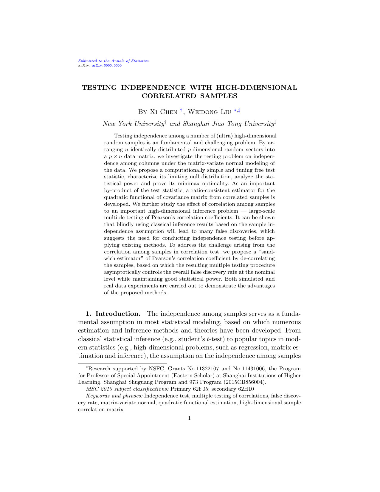 Figure 1
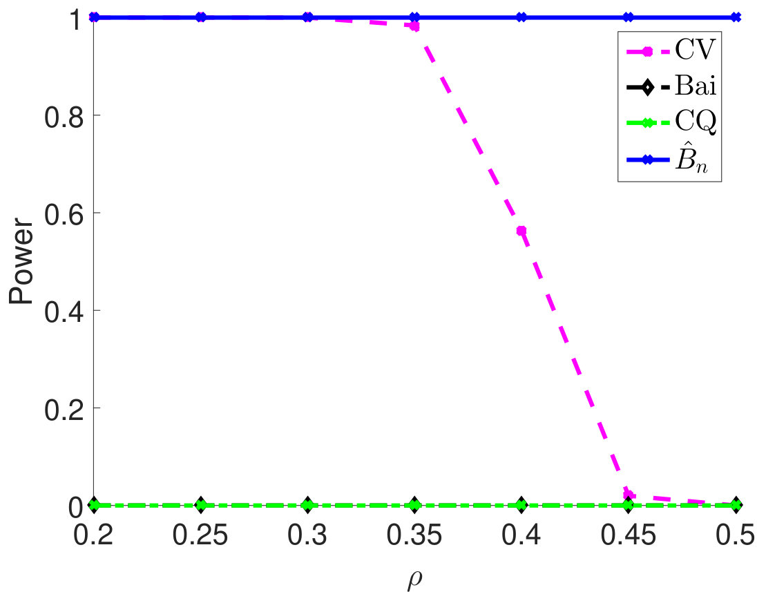 Figure 2
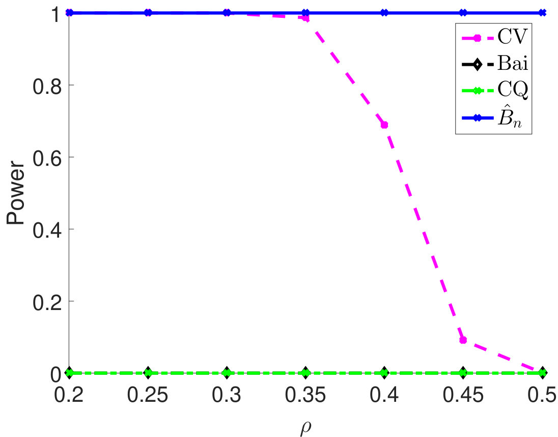 Figure 3
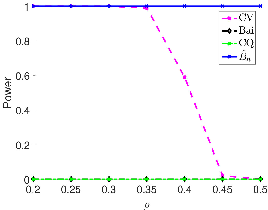 Figure 4
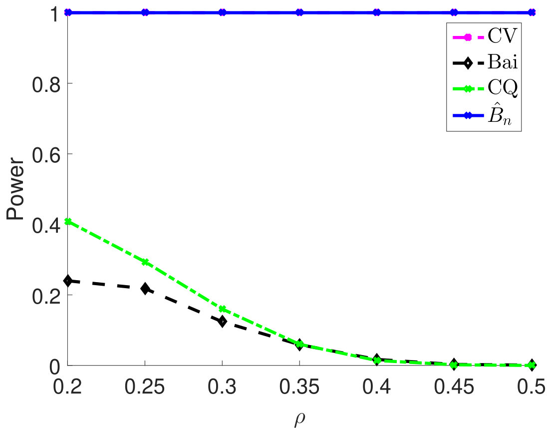 Figure 5
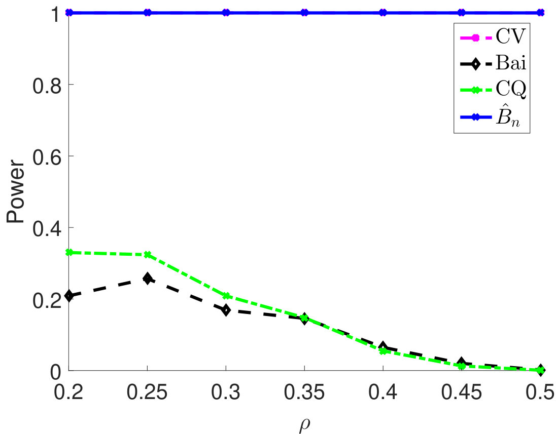 Figure 6
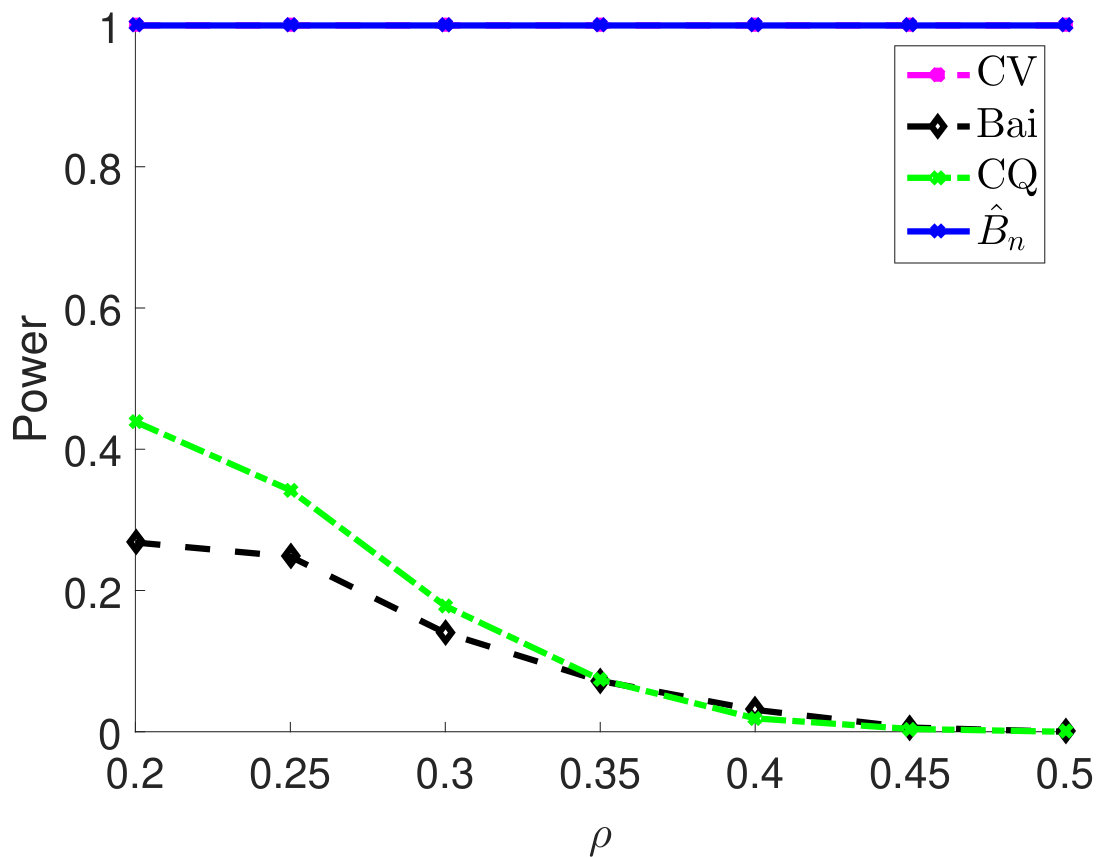 Figure 7
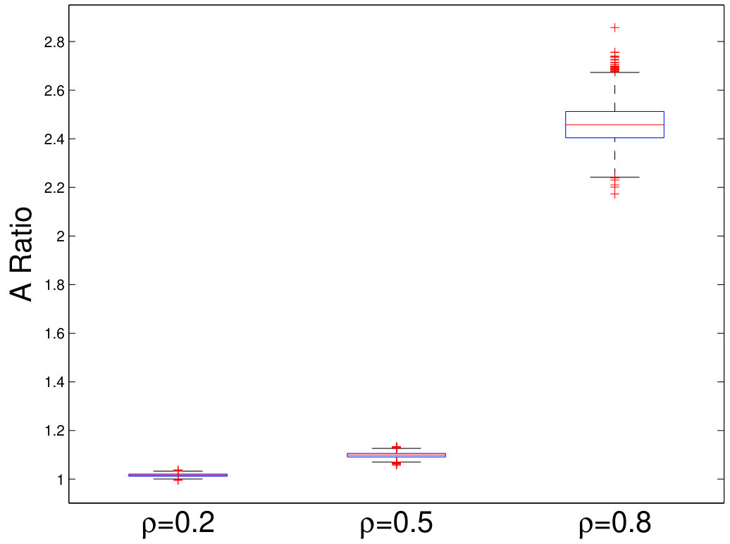 Figure 8
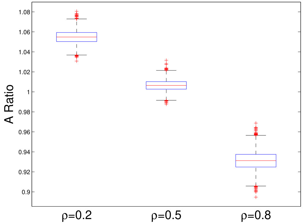 Figure 9
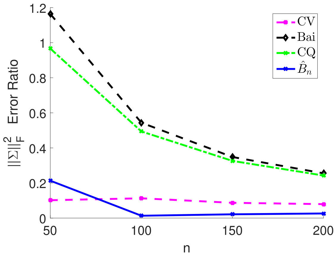 Figure 10
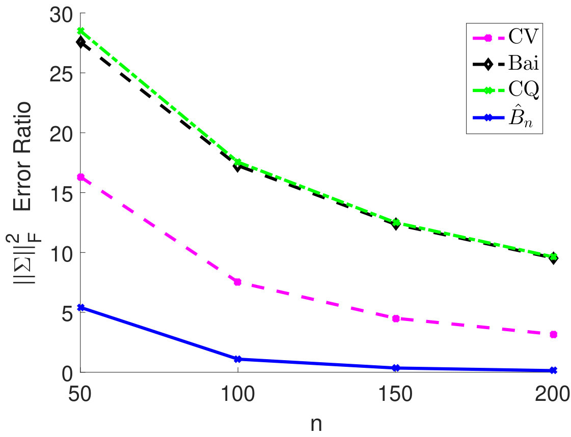 Figure 11
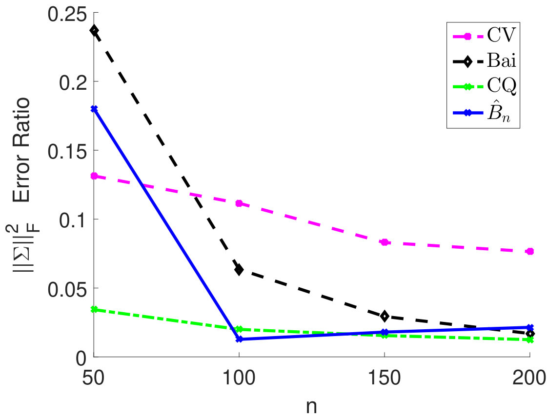 Figure 12
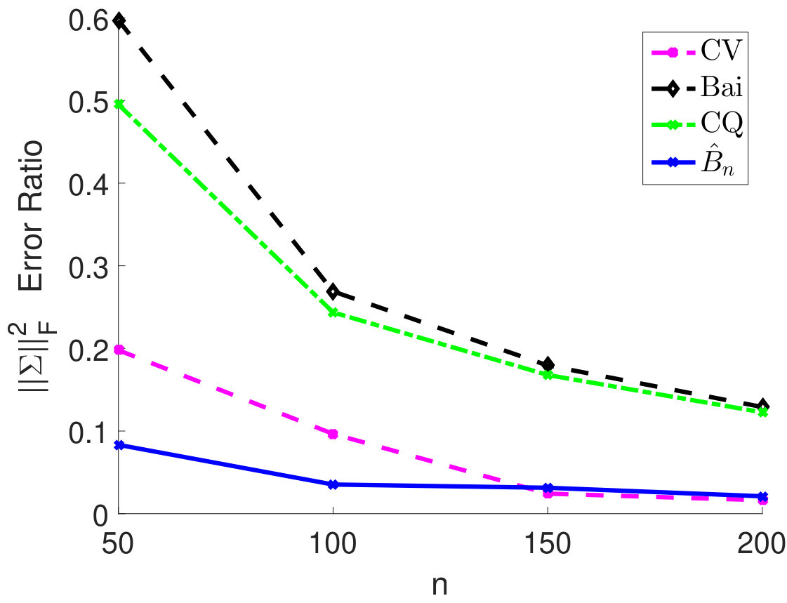 Figure 13
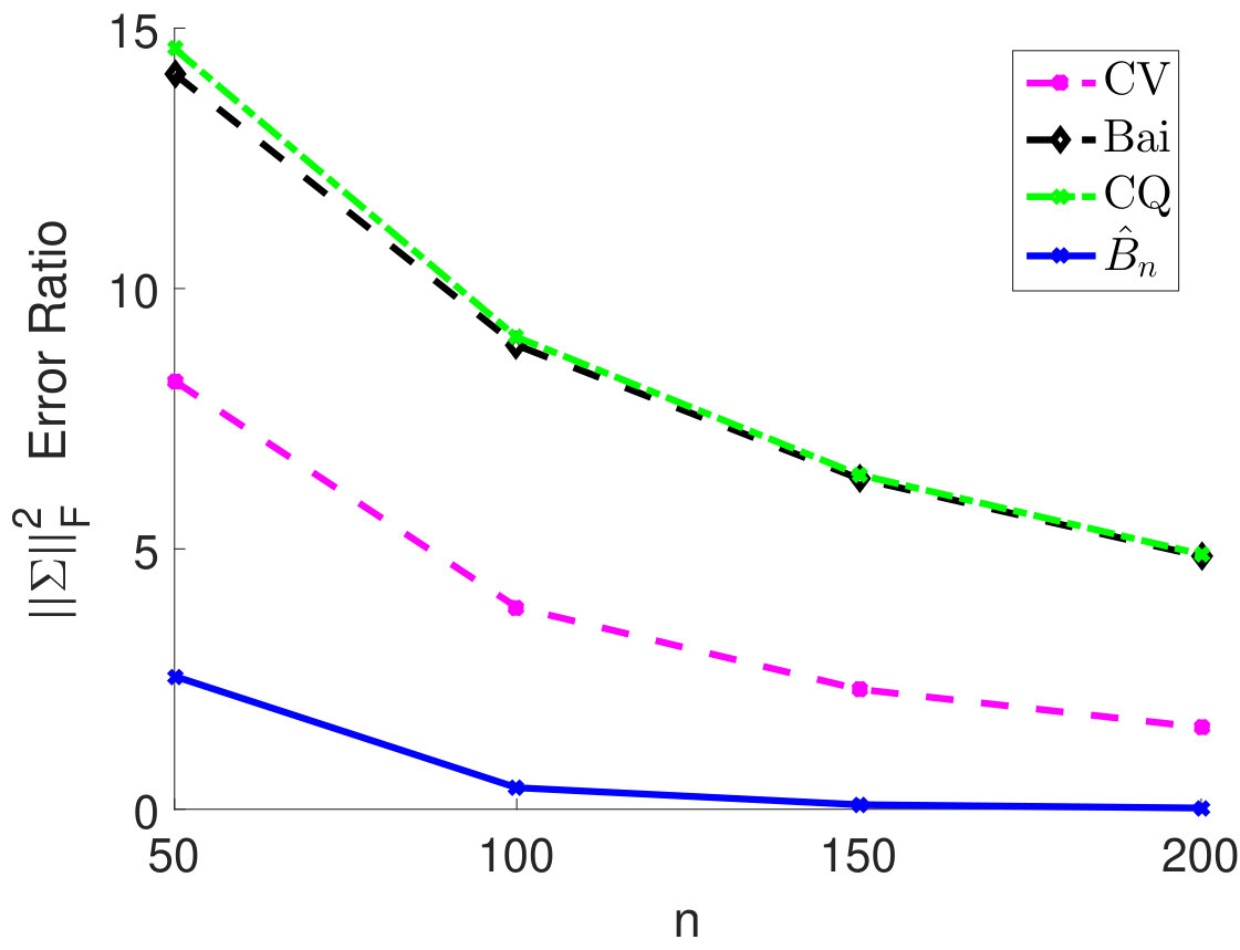 Figure 14
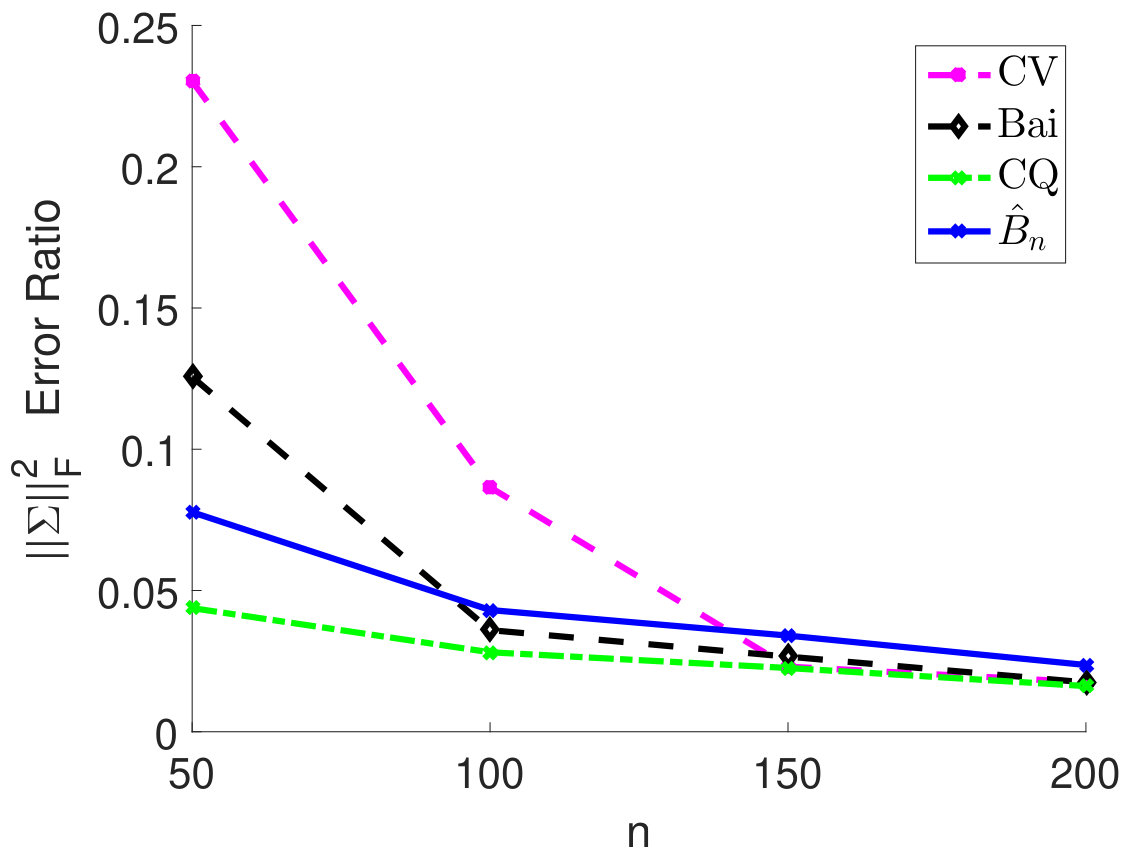 Figure 15
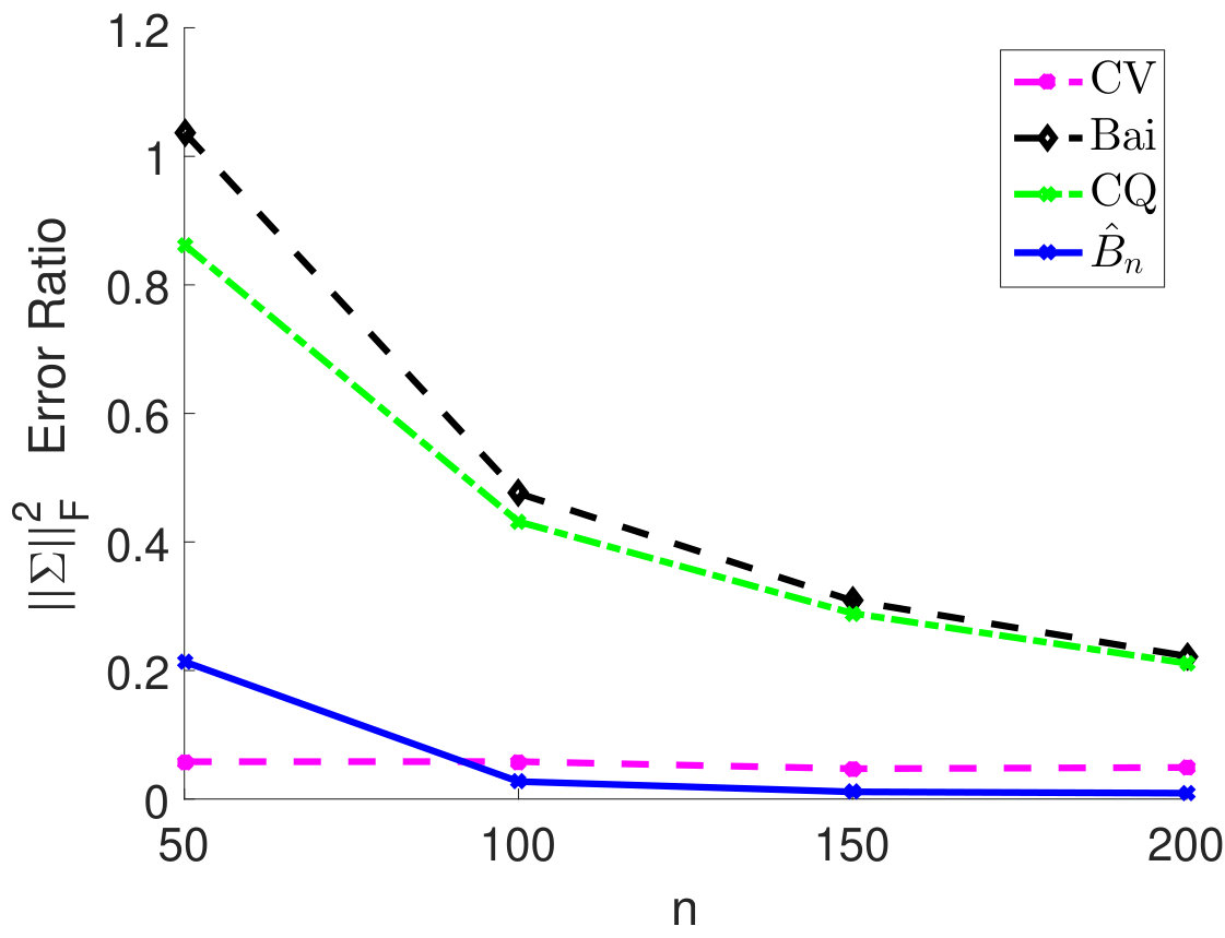 Figure 16
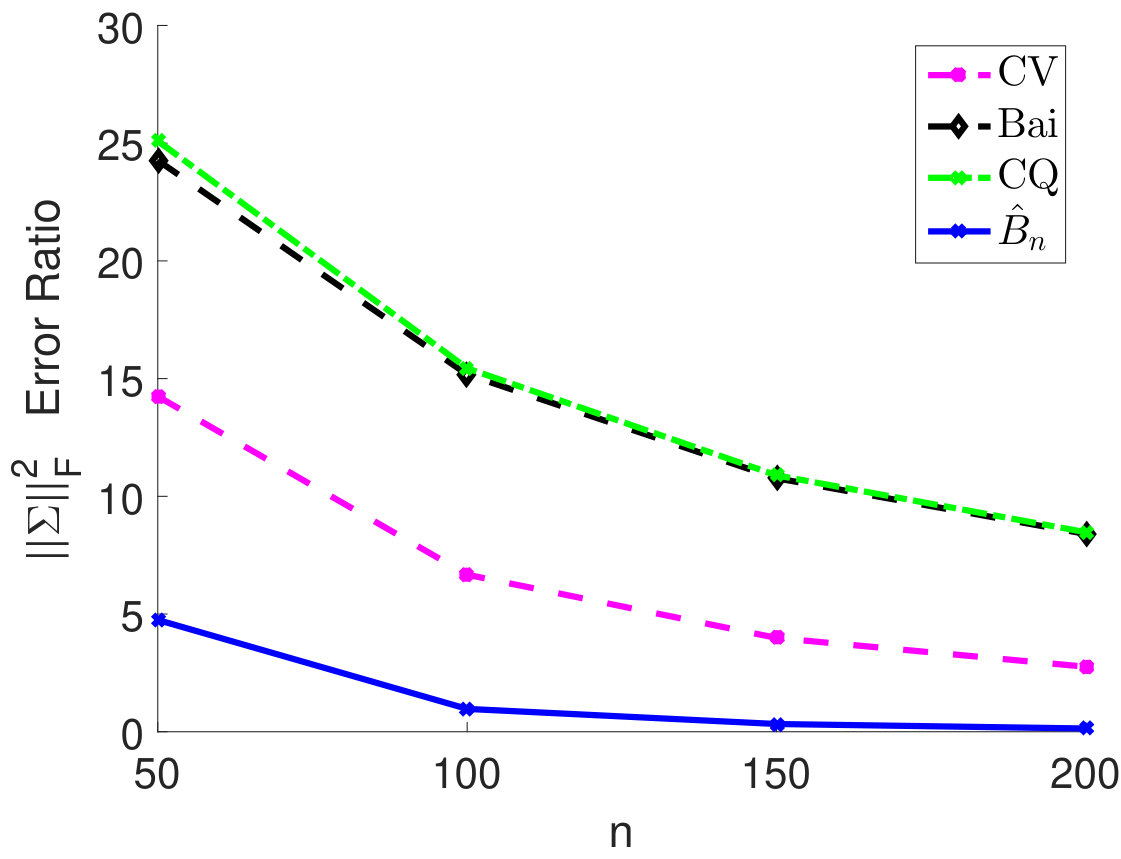 Figure 17
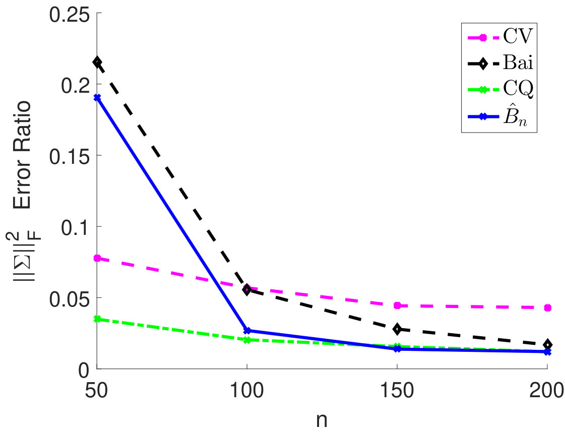 Figure 18
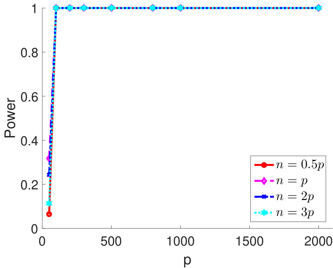 Figure 19
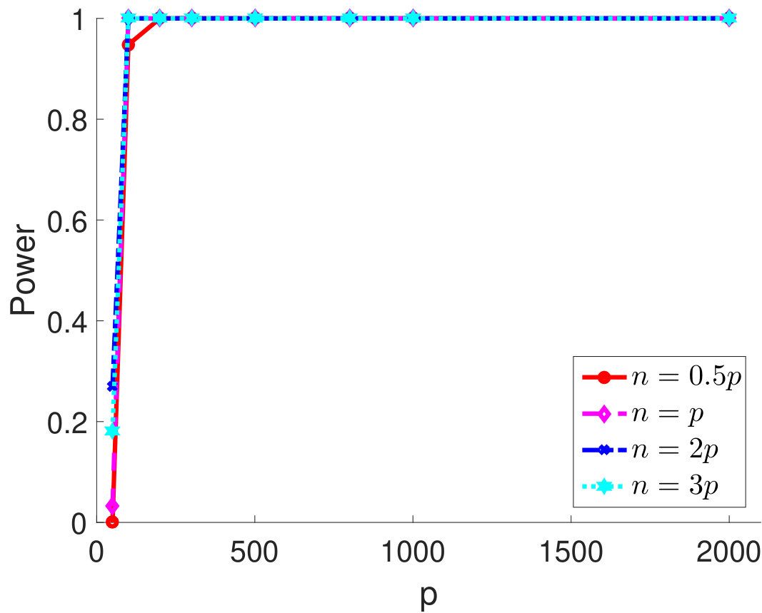 Figure 20
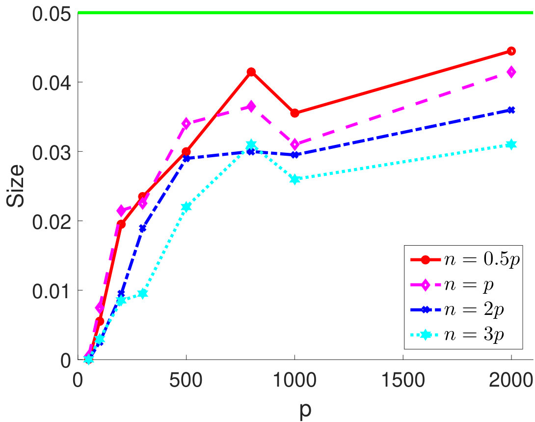 Figure 21
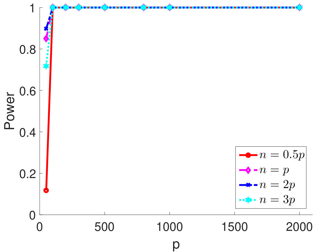 Figure 22
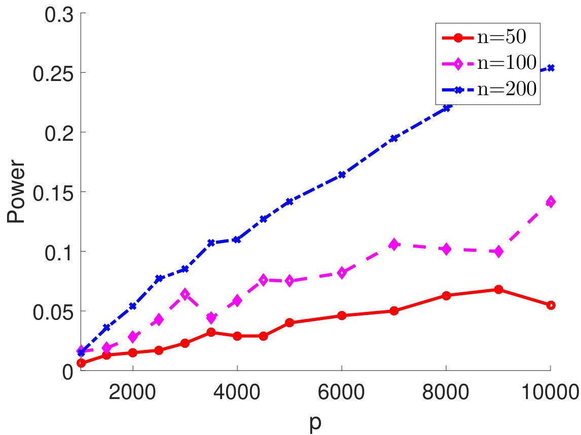 Figure 23
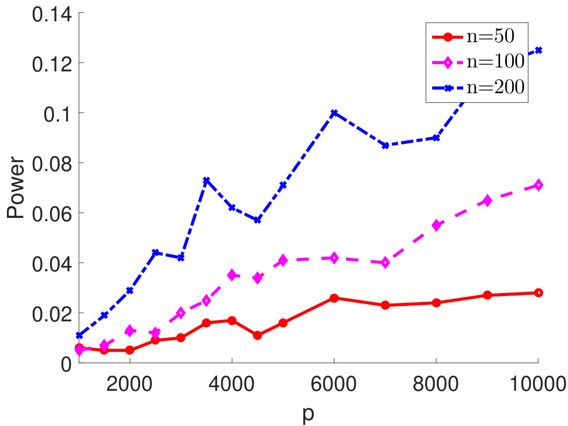 Figure 24
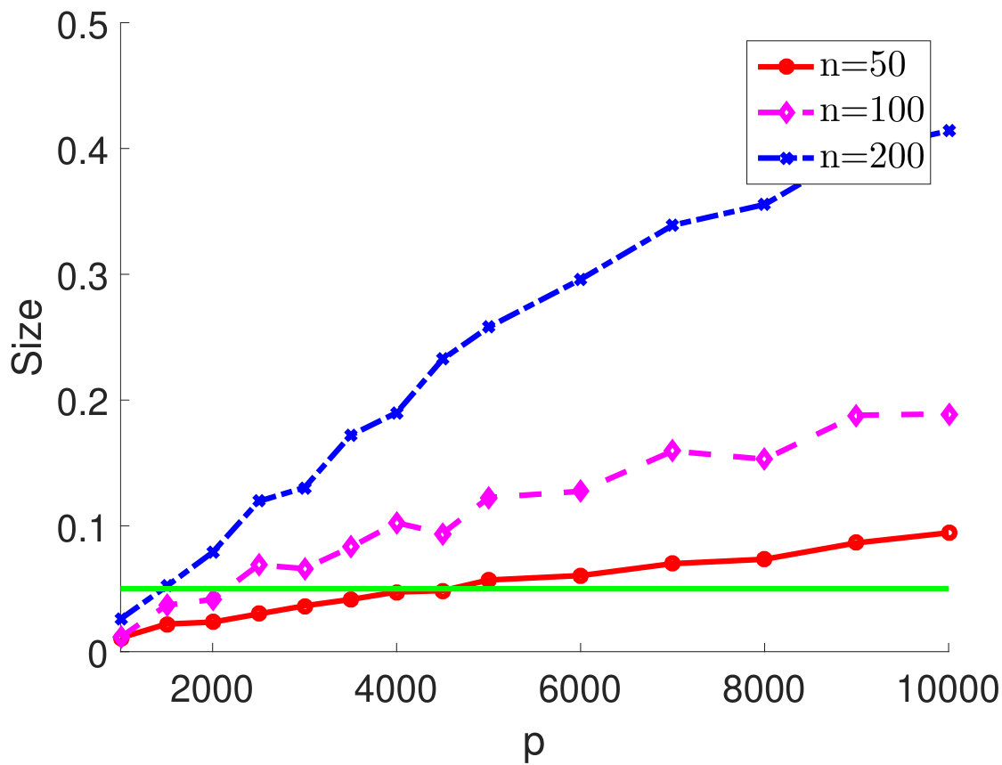 Figure 25
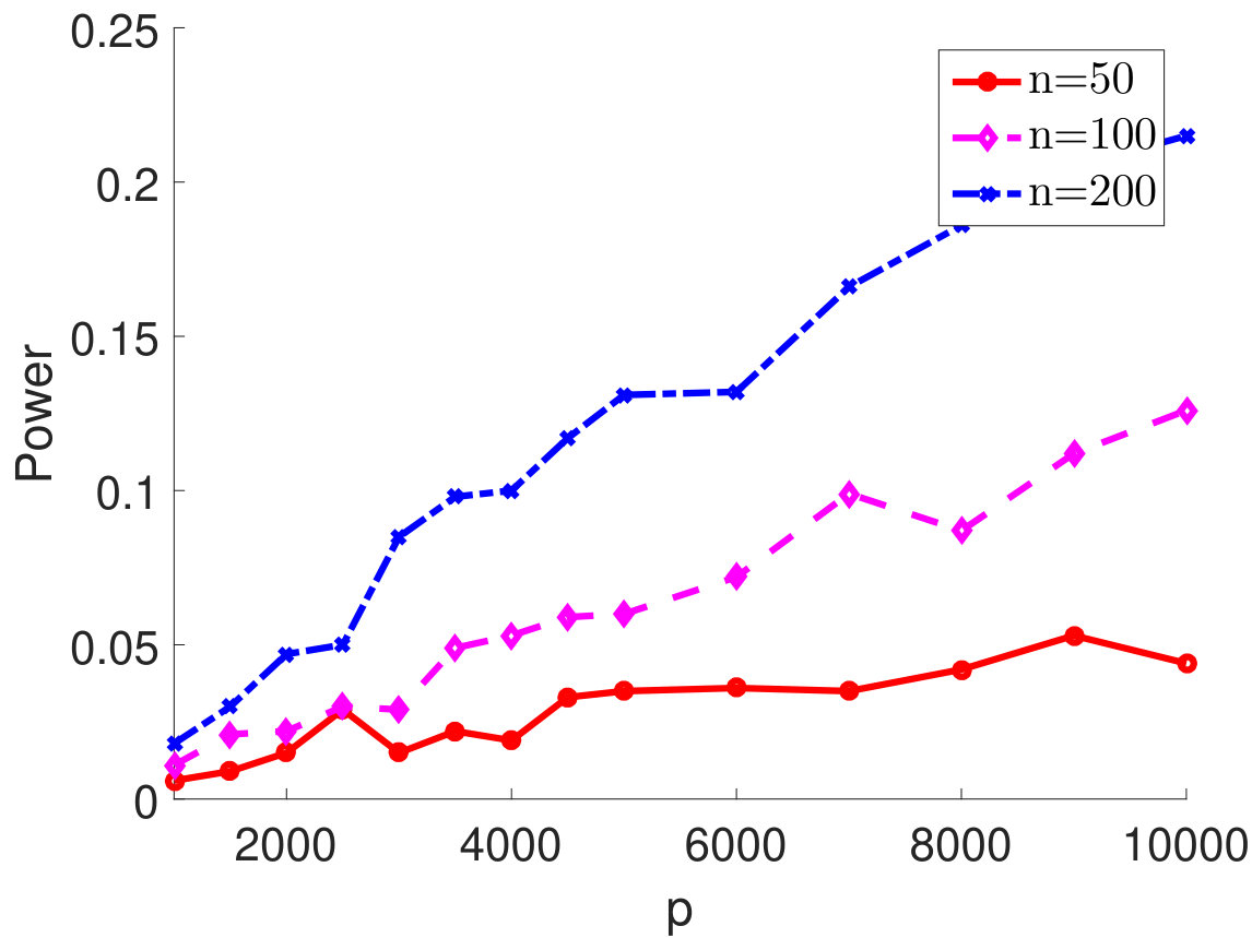 Figure 26
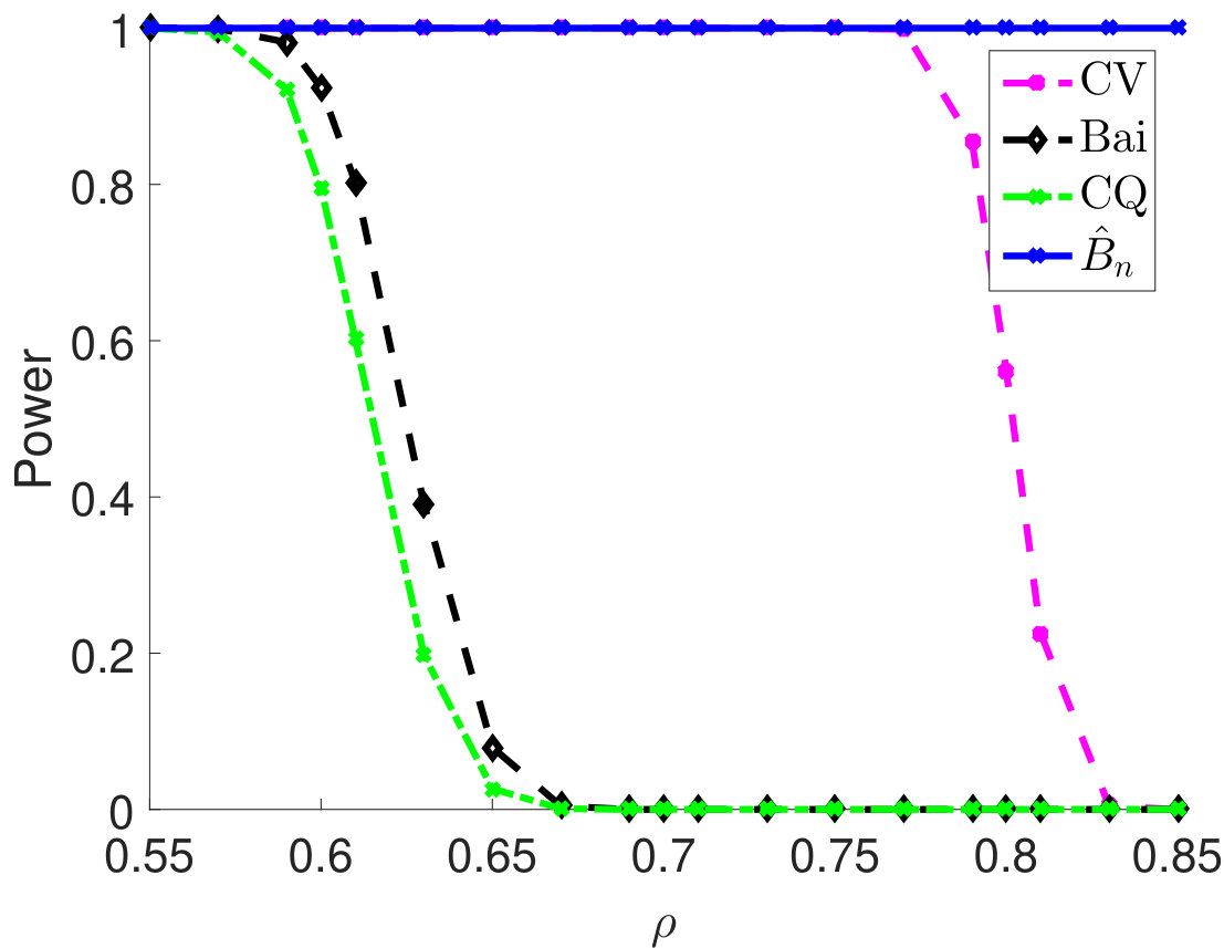 Figure 27
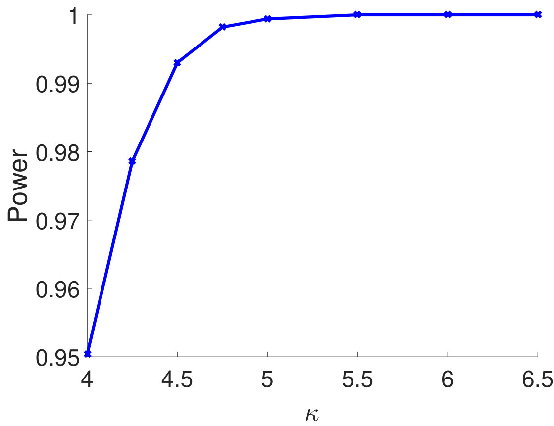 Figure 28
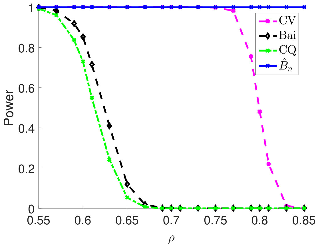 Figure 29
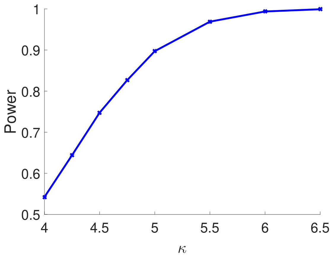 Figure 30
 Figure 31
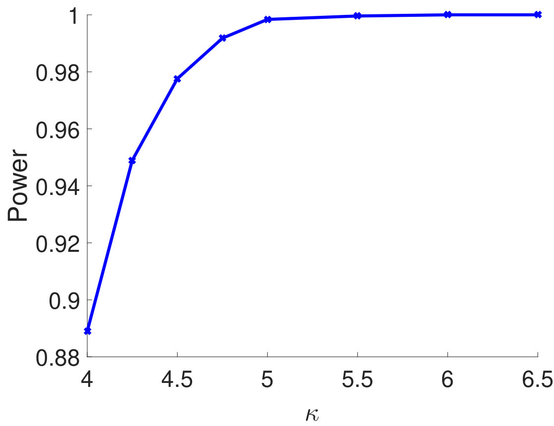 Figure 32
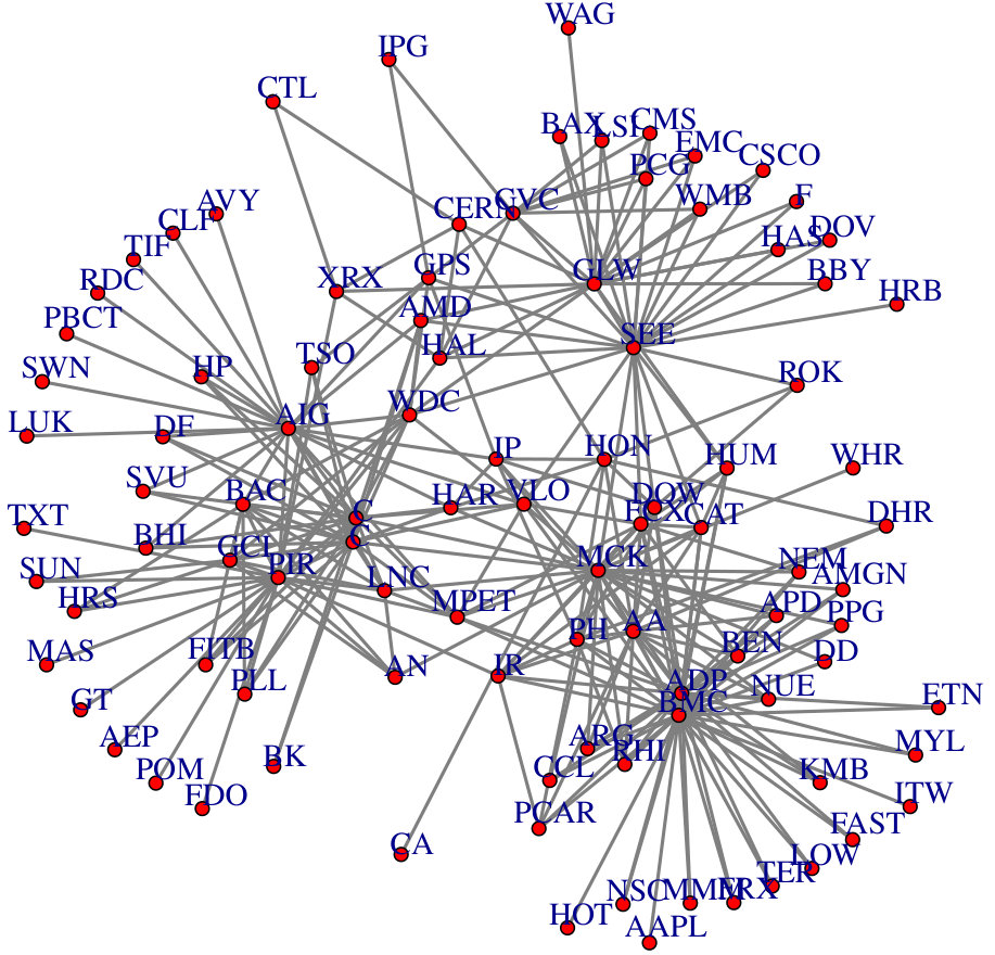 Figure 33
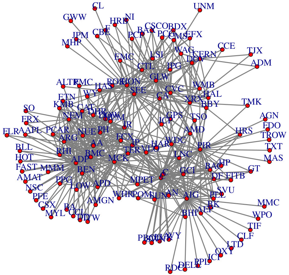 Figure 34
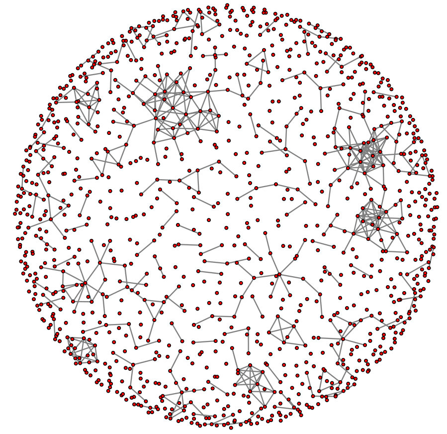 Figure 35
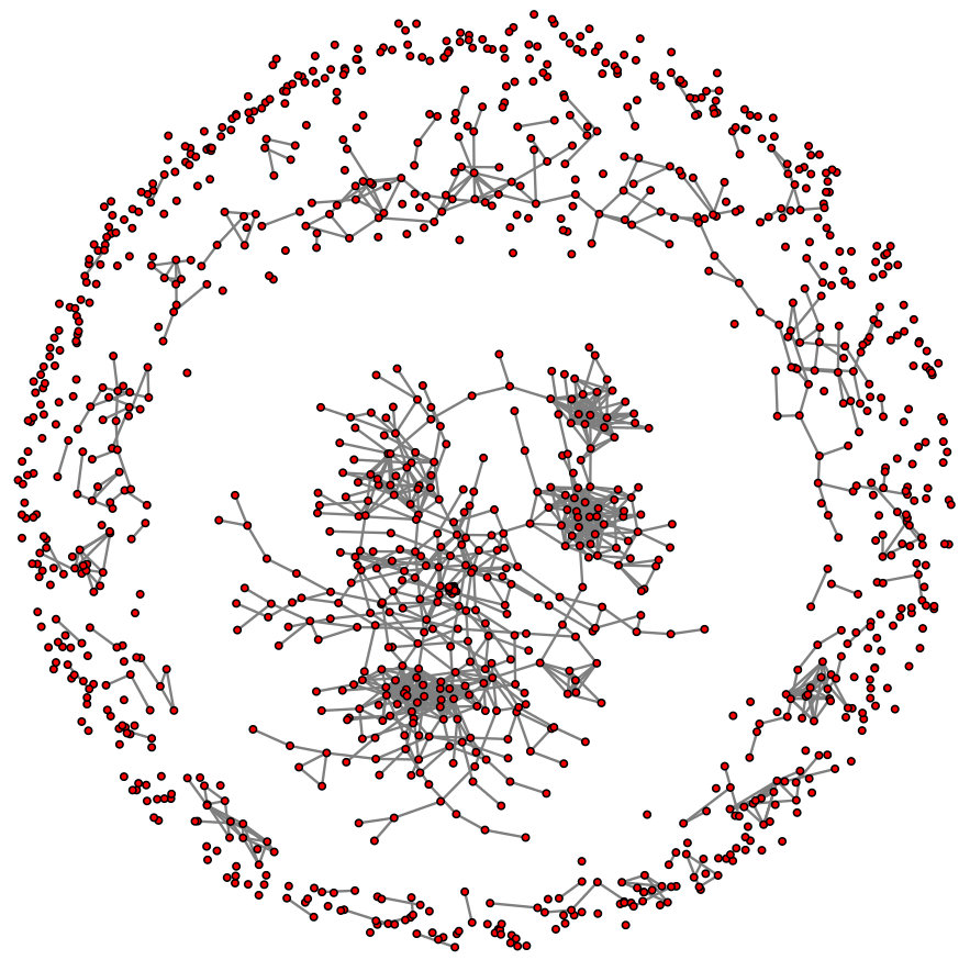 Figure 36
| 200 | 0.046 | 0.046 | 0.042 | 0.043 | ||
|---|---|---|---|---|---|---|
| 0.040 | 0.049 | 0.049 | 0.050 | |||
| 0.045 | 0.048 | 0.055 | 0.058 | |||
| band | 0.031 | 0.032 | 0.035 | 0.043 | ||
| block | 0.014 | 0.025 | 0.030 | 0.035 | ||
| 500 | 0.034 | 0.041 | 0.042 | 0.046 | ||
| 0.037 | 0.046 | 0.041 | 0.049 | |||
| 0.028 | 0.050 | 0.048 | 0.055 | |||
| band | 0.032 | 0.035 | 0.038 | 0.040 | ||
| block | 0.016 | 0.025 | 0.041 | 0.044 | ||
| 1000 | 0.039 | 0.035 | 0.048 | 0.044 | ||
| 0.035 | 0.042 | 0.056 | 0.054 | |||
| 0.026 | 0.040 | 0.051 | 0.050 | |||
| band | 0.029 | 0.037 | 0.040 | 0.045 | ||
| block | 0.016 | 0.024 | 0.035 | 0.041 |
| CV | Bai | CQ | ||||
|---|---|---|---|---|---|---|
| 50 | 0.029 | 0.001 | 0.038 | 0.002 | ||
| 0.129 | 0.004 | 0.039 | 0.008 | |||
| 0.157 | 0.010 | 0.022 | 0.037 | |||
| band | 0.072 | 0.005 | 0.033 | 0.007 | ||
| block | 0.249 | 0.011 | 0.028 | 0.017 | ||
| 100 | 0.070 | 0.017 | 0.041 | 0.028 | ||
| 0.118 | 0.020 | 0.036 | 0.034 | |||
| 0.101 | 0.019 | 0.025 | 0.049 | |||
| band | 0.066 | 0.017 | 0.034 | 0.025 | ||
| block | 0.068 | 0.017 | 0.023 | 0.016 |
| True | ||||||||||
|---|---|---|---|---|---|---|---|---|---|---|
| FDP | Power | FDP | Power | FDP | Power | FDP | Power | |||
| 50 | band | 0.010 | 0.311 | 0.027 | 0.339 | 0.010 | 0.276 | 0.015 | 0.339 | |
| band | 0.009 | 0.308 | 0.403 | 0.378 | 0.000 | 0.000 | 0.015 | 0.340 | ||
| band | 0.009 | 0.292 | 0.986 | 0.648 | 0.000 | 0.000 | 0.014 | 0.338 | ||
| block | 0.011 | 0.262 | 0.036 | 0.416 | 0.014 | 0.295 | 0.021 | 0.407 | ||
| block | 0.011 | 0.257 | 0.366 | 0.504 | 0.000 | 0.000 | 0.021 | 0.410 | ||
| block | 0.012 | 0.168 | 0.965 | 0.739 | 0.010 | 0.000 | 0.021 | 0.408 | ||
| 100 | band | 0.025 | 0.576 | 0.057 | 0.593 | 0.029 | 0.568 | 0.033 | 0.587 | |
| band | 0.025 | 0.575 | 0.581 | 0.650 | 0.011 | 0.448 | 0.032 | 0.587 | ||
| band | 0.025 | 0.556 | 0.986 | 0.795 | 0.000 | 0.000 | 0.032 | 0.587 | ||
| block | 0.028 | 0.942 | 0.061 | 0.961 | 0.035 | 0.945 | 0.038 | 0.966 | ||
| block | 0.028 | 0.935 | 0.454 | 0.942 | 0.017 | 0.646 | 0.038 | 0.966 | ||
| block | 0.030 | 0.820 | 0.963 | 0.924 | 0.000 | 0.000 | 0.038 | 0.966 | ||
| 200 | band | 0.036 | 0.839 | 0.072 | 0.852 | 0.039 | 0.820 | 0.041 | 0.854 | |
| band | 0.036 | 0.835 | 0.620 | 0.867 | 0.028 | 0.640 | 0.041 | 0.853 | ||
| band | 0.041 | 0.749 | 0.984 | 0.906 | 0.002 | 0.240 | 0.042 | 0.852 | ||
| block | 0.034 | 1.000 | 0.071 | 1.000 | 0.041 | 1.000 | 0.043 | 1.000 | ||
| block | 0.034 | 1.000 | 0.498 | 1.000 | 0.033 | 0.992 | 0.044 | 1.000 | ||
| block | 0.040 | 0.969 | 0.962 | 0.994 | 0.004 | 0.233 | 0.044 | 1.000 | ||
| FDP | Power | FDP | Power | ||||
|---|---|---|---|---|---|---|---|
| 50 | band | 0.009 | 0.318 | 0.014 | 0.341 | ||
| block | 0.012 | 0.293 | 0.021 | 0.408 | |||
| 100 | band | 0.025 | 0.578 | 0.032 | 0.587 | ||
| block | 0.028 | 0.952 | 0.037 | 0.965 | |||
| 200 | band | 0.035 | 0.844 | 0.041 | 0.852 | ||
| block | 0.035 | 1.000 | 0.043 | 1.000 | |||
| 50 | 0.004 | ||
| 0.013 | |||
| 0.047 | |||
| band | 0.010 | ||
| block | 0.025 | ||
| 100 | 0.039 | ||
| 0.043 | |||
| 0.058 | |||
| band | 0.031 | ||
| block | 0.023 |
| No. of Rejections | 448 | 1062 | 2114 | 154072 | 220390 | 294810 |
|---|---|---|---|---|---|---|
| Density (%) | 0.07% | 0.15% | 0.29% | 21.17% | 30.28% | 40.51% |
| No. of Rejections | 287 | 442 | 1034 | 873 | 1263 | 2751 |
|---|---|---|---|---|---|---|
| Density (%) | 0.87% | 1.69% | 3.12% | 2.63% | 4.58% | 8.30% |
| Stock 1 | GICS of Stock 1 | Stock 2 | GICS of Stock 2 |
|---|---|---|---|
| American International Group | Financials | Citigroup | Financials |
| Corning | Industrials | Sealed Air Corp | Materials |
| Automatic Data Processing | Internet Software & Services | BMC Software | Internet Software & Services |
| Bank of America Corp | Financials | Citigroup | Financials |
| BMC Software | Internet Software & Services | McKesson | Health Care |
Peer Reviews
No public reviews on file for this paper yet. If you reviewed it on a platform where reviews are public (OpenReview, ICLR, NeurIPS, ICML), you can paste yours below so the community can read it here.
Videos
No videos yet. Explain this paper in a talk, walkthrough, or lecture? Add one.
Taxonomy
TopicsRandom Matrices and Applications · Statistical Methods and Inference · Statistical Methods and Bayesian Inference
Testing independence with high-dimensional correlated samples
Xi Chen label=e1][email protected] [
Weidong Liu label=e2][email protected] [ New York University\thanksmarkm1 and Shanghai Jiao Tong University\thanksmarkm2
Stern School of Business
New York University
44 West 4th Street
New York, NY, USA
Department of Mathematics
Institute of Natural Sciences and Moe-LSC
Shanghai Jiao Tong University
Shanghai, China
Abstract
Testing independence among a number of (ultra) high-dimensional random samples is a fundamental and challenging problem. By arranging identically distributed -dimensional random vectors into a data matrix, we investigate the problem of testing independence among columns under the matrix-variate normal modeling of data. We propose a computationally simple and tuning-free test statistic, characterize its limiting null distribution, analyze the statistical power and prove its minimax optimality. As an important by-product of the test statistic, a ratio-consistent estimator for the quadratic functional of a covariance matrix from correlated samples is developed. We further study the effect of correlation among samples to an important high-dimensional inference problem — large-scale multiple testing of Pearson’s correlation coefficients. Indeed, blindly using classical inference results based on the assumed independence of samples will lead to many false discoveries, which suggests the need for conducting independence testing before applying existing methods. To address the challenge arising from correlation among samples, we propose a “sandwich estimator” of Pearson’s correlation coefficient by de-correlating the samples. Based on this approach, the resulting multiple testing procedure asymptotically controls the overall false discovery rate at the nominal level while maintaining good statistical power. Both simulated and real data experiments are carried out to demonstrate the advantages of the proposed methods.
62F05,
62H10 ,
Independence test,
multiple testing of correlations,
false discovery rate,
matrix-variate normal,
quadratic functional estimation,
high-dimensional sample correlation matrix,
keywords:
[class=MSC]
keywords:
,
t1Research supported by NSFC, Grants No.11322107 and No.11431006, the Program for Professor of Special Appointment (Eastern Scholar) at Shanghai Institutions of Higher Learning, Shanghai Shuguang Program and 973 Program (2015CB856004).
1 Introduction
The independence among samples is a fundamental assumption in most statistical modeling upon which numerous estimation and inference methods and theories have been developed. Indeed, from classical statistical inference (e.g., student’s -test) to popular topics in modern statistics (e.g., high-dimensional problems, such as regression, matrix estimation and inference), this assumption of independence occurs widely. Consider samples , where each sample is a -dimensional vector from the same population distribution with mean and covariance . It is often convenient to pool samples together to form a data matrix . More specifically, for example in microarray data, X is an expression level matrix for genes measured on subjects. Such data are usually high-dimensional; thus, we mainly consider the setting where is much larger than . Most existing works in high-dimensional literature make the independence assumption among columns of X, serving as the starting point of methodology development and technical analysis. However, recent studies have shown that there are correlation structures among subjects in various microarray datasets (see, e.g., Teng and Huang (2009); Efron (2009); Allen and Tibshirani (2012); Kim et al. (2012)), demonstrating the potential risk of making the seemingly natural assumption of independence. Therefore, given a data matrix , it is important to first test whether the samples are indeed independent before applying any method that assumes independence.
A data matrix is known as transposable data when both rows and columns are potentially correlated (Lazzeroni and Owen, 2002; Allen and Tibshirani, 2012). For a transposable data matrix X, it is commonly assumed that X follows a matrix-variate normal distribution, which has been widely applied to model microarray data (see, e.g., Teng and Huang (2009); Efron (2009); Muralidharan (2010); Allen and Tibshirani (2012); Yin and Li (2012); Kim et al. (2012); Zhou (2014)). The matrix-variate normal distribution is a natural generalization of familiar vector-variate normal distribution (Dawid, 1981). In particular, let be the vectorization of matrix obtained by stacking the columns of on top of each other. We say follows a matrix-variate normal distribution with the mean matrix and covariance matrix (denoted by ) if and only if . Here, denotes the transpose of X, is the Kronecker product, and is the covariance matrix of row vectors of X. Given a matrix-variate normal , each column for , where is the -th column of the mean matrix M. Recall our problem setup: each follows the same population distribution with mean vector and covariance . Thus, we have where 1 is the -dimensional all one column vector and for . Under the matrix-variate normal modeling of the data, the independence testing problem is equivalent to the global test of whether is a diagonal matrix, i.e.,
[TABLE]
The testing problem in (1) is closely related to the following correlation test problem
[TABLE]
where is the Pearson’s correlation coefficient. The testing problem in (2) is a classical problem in multivariate analysis (Nagao, 1973; Anderson, 2003). It has also been extensively studied in the past decade under the high-dimensional setting (e.g., Johnstone (2001), Ledoit and Wolf (2002), Jiang (2004), Schott (2005), Liu, Lin and Shao (2008), Bai et al. (2009), Cai and Jiang (2011), Jiang and Yang (2013), Han and Liu (2014)). However, the reported results are based on the assumption that samples are independent. In fact, our problem in (1) is equivalent to the testing problem (2) with correlated samples. To see this, note that when treating each row of X as an individual sample, the role of and interchanges since , i.e., the matrix models the correlations among row samples while becomes the population covariance matrix. For many types of data (e.g., genetic data, financial data), there exists a complicated correlation structure among variables. Thus, will not be a diagonal matrix and row vectors are not independent. Our problem in (1) essentially tests the correlation among row vectors when samples are correlated. The correlation among samples makes our problem more challenging; and the aforementioned methods for testing (2), which are based on the assumption of sample independence, cannot be applied to our problem.
The classical methods for testing independence among samples commonly assume is fixed and are usually designed only for time series data. It is also known as serial independence test, see Hong (1998) and the references therein. In such a framework, the methods require that the samples under alternatives come from some time series. These samples satisfy an ordering structure such that the dependence between two samples decays as the distance of their indices increases. In our setting, there is no structural assumption among samples. Without any structural assumption, we will show in Theorem 2.7 that any test will not have the power tending to 1 uniformly over a large class of alternatives when the dimension is small (e.g., fixed constant or ). On the other hand, for but is small compared to , the independence test is relatively easy. In fact, if is known, the data matrix can be transformed as ; and thus the independence test can be directly carried out using existing approaches (e.g., Jiang (2004); Liu, Lin and Shao (2008)). One can apply such an approach with a plug-in estimator . However, as we will explain later in Section 5, when , even the optimal convergence rate of the estimator is not fast enough to solve this problem. In fact, although we have more information (i.e., row samples) as becomes larger, the number of unknown parameters in increases accordingly, which makes the problem challenging. Therefore, the high-dimensional setting is the most interesting case, and will be the main focus of the paper.
Although the testing of independence among high-dimensional samples is an important and fundamental problem, few existing works have done so. Based on matrix-variate normal modeling of the data, some inference approaches were proposed by Efron (2009) and Muralidharan (2010). However, these works do not explore the limiting null distributions as well as the validity and power of the test. Pan, Gao and Yang (2014) proposed a statistic for this problem based on random matrix theory. However, it requires the condition that is proportionally as large as (i.e., ), and thus cannot be applied to cases where with or, as in the ultra high-dimensional setting, where for some ; both scenarios are common in genetic applications. Further, the method in Pan, Gao and Yang (2014) requires splitting samples into two parts and differences in splitting could lead to different test results.
In this paper, we consider the (ultra) high-dimensional setup and propose a minimax optimal test procedure in terms of the statistical power for the testing problem in (1). We show that the distribution of the proposed max-type test statistic converges to a type I extreme value distribution under the null (Theorem 2.4). Therefore, the proposed test has the pre-specified significance level asymptotically. We also investigate the statistical power. Roughly speaking, we show that under some very mild conditions on off-diagonal elements of , the power will converge to 1. Further, we prove that the proposed test is minimax rate-optimal over a large class of (Theorems 2.5 and 2.6).
Our construction of the test statistic combines a bias correction and a variance correlation based on the sample covariance matrix , where we treat each row of X as a sample. The bias correction technique allows us to handle the ultra high-dimensional case. Moreover, the variance correlation technique deals with the correlation structure among “row samples” of X, which is specified by . To characterize the strength of correlation among row samples, we identify a key quantity , which comes from the asymptotic variance of our bias-corrected statistic. Here, denotes the Frobenius norm and is the trace of . To simultaneously control the type I error under null and maintain the minimax rate-optimal statistical power, we need a ratio consistent estimator of regardless of the correlation among samples. Therefore, the remaining task essentially reduces to the problem of estimating from correlated samples.
It is noteworthy that estimating itself is an important problem, which is known as quadratic functional estimation of (see, e.g., Bai and Saranadasa (1996); Chen and Qin (2010); Fan, Rigollet and Wang (2015)). Most existing works are based on the assumption that samples are independent and identically distributed (i.i.d.) and, thus, cannot be directly applied to our problem. Motivated by the thresholding estimator in Fan, Rigollet and Wang (2015), we propose a plugin estimator for based on a thresholded sample covariance matrix but we relax the independence assumption among samples. Further, we propose a definite threshold level, which is adaptive to the amount of correlations among samples and guarantees the consistency of the resulting estimator. Our simulation results demonstrate the superior performance of the proposed estimator of over the existing approaches, which leads to a significant improvement in statistical power.
In summary, we propose a simple max-type test statistic to conduct the global test of independence among high-dimensional random samples in (1). Our approach has the following advantages:
Our construction is direct and computationally attractive, which only requires the row sample covariance matrix and a threshold estimator of . Further, our test statistic is completely tuning free. 2. 2.
The limiting null distribution is characterized and thus the type I error is controlled asymptotically. Further, our test procedure is minimax rate-optimal over a sufficiently large class of , which is enough for most practical purposes. 3. 3.
As an important by-product, we provide a ratio-consistent estimator for estimating quadratic functional of covariance matrix from correlated samples.
We would like to note that we only focus on the matrix-variate normal distribution, which is a common assumption for studying a transposable data matrix and widely used for modeling correlated microarray data. It is of interest to investigate the independence test for more general distributions, e.g., a matrix elliptical distribution (Dawid, 1977; Fang and Zhang, 1990) or , where entries of are i.i.d. random variables with unit variance. We leave the extension to such distributions of data matrices for future work.
After we conduct the independence test, if the samples are indeed correlated, many classical inference approaches cannot be directly applied. We use the multiple testing problem of Pearson’s correlation coefficients to illustrate the effect of the correlation among samples, demonstrate the reason why the classical approach will fail when samples are correlated and further develop a new method to de-correlate the samples. In particular, we consider the following large-scale multiple testing problem, for ,
[TABLE]
Problem (3) is a natural extension of the global test of independence in (2). In fact, the hypothesis that is a diagonal matrix is a strong null hypothesis, which will be rejected in most real data applications (e.g., microarray data, stock data). In contrast, the goal of the multiple testing problem (3) is to identity the pairs of correlated variables and thus find many applications in real data analysis, e.g., gene coexpression network analysis (Lee, Hsu and Sajdak, 2004; Carter et al., 2004; Zhu et al., 2005; Hirai, 2007), and brain connectivity analysis (Shaw, 2006). The goal of the testing problem in (3) is consistent with the goal of support recovery of a sparse . The latter problem has been extensively studied in recent years (e.g., see Rothman, Levina and Zhu (2009), Lam and Fan (2009), Cai and Liu (2011), Bien and Tibshirani (2011)). These works establish consistency results of support recovery from independent samples under certain conditions, for example, all the absolute values of nonzero are lower bounded by , which might be hard to hold in practice. Instead of trying to achieve the perfect support recovery, the multiple testing problem (3) has a more refined control of the type I error rate in support recovery under weaker assumptions. In particular, it usually aims to control the false discovery rate (FDR), which is a useful measure for evaluating the performance of support recovery. We also note that Cai and Liu (2015) recently studied problem (3) in a high-dimensional setting but it still requires the independence assumption.
For correlated samples from a matrix-variate normal distribution, we first establish the following result on the limiting distribution of the sample correlation coefficient (see Proposition 3.1):
[TABLE]
where , which quantifies the strength of the correlation among samples. Eq. (4) subsumes as a special case the classical results on the limiting distribution of when samples are i.i.d. ( in (4)) (see Theorem 4.2.4 in Anderson (2003)). When the correlation is strong to a certain extent such that for some constant , directly using sample correlation coefficient or Fisher’s statistic will lead to many false positives; this is verified by our simulations in Section 4.2. In fact, even if is known and one uses the correct limiting null distribution of , the variance of becomes larger as increases, which leads to a lower power of the test.
To overcome the side effect of correlation among samples, we propose a “sandwich estimator” of by de-correlating the samples, which has the limiting distribution . The corresponding asymptotical variance does not depend on and is smaller than that of the naïve estimator . Therefore the proposed “sandwich estimator” has an improved statistical power especially when the correlation among samples is strong. Based on the proposed “sandwich estimator” of , the standard multiple testing procedure (Benjamini and Hochberg, 1995) is proven to asymptotically control the FDR at the nominal level (see Theorem 3.2).
Finally, we introduce some necessary notations. For a positive integer , . For a square matrix , let denote the trace of , the maximum eigenvalue of , and the minimum eigenvalue of . Let be the indicator function that takes value one when the event is true and zero otherwise. For a given set , let be the cardinality of . For any two real numbers and , let and . We use and to denote limit superior and limit inferior, respectively. Throughout the paper, we use to denote the identity matrix, and use , , , etc. to denote constants for which values might change from place to place and do not depend on and .
The rest of the paper is organized as follows. In Section 2, we study the global test in (1). The test statistic is proposed in Section 2.1. In Section 2.2, we provide the ratio consistent estimator of and from correlated samples. The estimation error is characterized in Theorem 2.1. We further provide the limiting null distribution of the test statistic and the power analysis (Theorems 2.4–2.7). Section 3 studies the multiple testing of correlations in (3) from correlated samples. Experimental results are given in Section 4 followed by discussion in Section 5. The proofs of our results as well as some additional experimental results are provided in Appendix.
2 Sample independence test
We study the global testing problem of sample independence in (1) given the data matrix .
2.1 Construction of the test statistic
Recall that denotes the -th sample for and let . Define
[TABLE]
In fact, from the proof, the statistic is the sample covariance coefficient corresponding to . Further, under the null , we can show that
[TABLE]
The first term has mean and variance . The bias term comes from the centralization statistics in (5). When , we have and can be shown to converge to a normal distribution. However, as we are interested in the ultra high-dimensional case where can be as large as for some , when becomes larger such that , in probability under the null. To enable the applicability of our test statistic in the ultra high-dimensional setting, we first propose the following bias corrected quantity:
[TABLE]
where is the sample variance corresponding to . Since the first term in (6) has variance , the asymptotic variance of is , where
[TABLE]
quantifies the strength of correlations among row vectors of X.
Given in (8), we will show that under the null as ,
[TABLE]
for , where the term plays the role of variance correction for . The remaining task is to develop a ratio consistent estimator for . In addition, to maintain the statistical power, the estimator should also be consistent for correlated samples. In Section 2.2, we will develop such an estimator for . Given the estimator (see (14)), we propose the following test statistic for the independence test in (1),
[TABLE]
2.2 Estimation of and from correlated samples
The estimation of finds many applications and has been studied in several works (Bai and Saranadasa, 1996; Chen and Qin, 2010; Fan, Rigollet and Wang, 2015). However, all these works rely on the sample independence assumption. In particular, Fan, Rigollet and Wang (2015) proved that the simple plug-in procedure based on threshold estimators are minimax optimal over a large class of covariance matrices. Moreover, the threshold level in Fan, Rigollet and Wang (2015) takes the form of , where the constant needs to be carefully tuned to achieve good performance in practice. A cross-validation (CV) procedure was suggested; however, there is no theoretical justification for such a CV procedure. In this section, we introduce a threshold estimator for with an explicit threshold level, which is completely data-driven without any tuning and automatically adaptive to the correlation among samples. We will show in Theorem 2.1 that the obtained estimator is ratio-consistent for correlated samples.
Let us define the (column) sample covariance matrix with and sample correlation coefficient for . Further, define
[TABLE]
which quantifies the average correlation among samples. It can be shown that (see Proposition 3.1 in Section 3 and note that in probability). We propose the following threshold estimator , where
[TABLE]
Here, is an estimator of and can be any constant larger than . Let . Using the approach from Bai and Saranadasa (1996), we construct
[TABLE]
Given the threshold estimator in (12), the is estimated by and is estimated by
[TABLE]
Now we will show that and are ratio-consistent estimators of and , respectively. We first make the following three assumptions throughout this section. Let be the eigenvalues of and be eigenvalues of . We make the following standard assumption on eigenvalues:
(C1) We assume that and for some constant .
The condition (C1) is a typical eigenvalue assumption in high-dimensional covariance estimation literature (see the survey Cai, Ren and Zhou (2016) and references therein). This assumption is natural for many important classes of covariance matrices, e.g., bandable, Toeplitz, and sparse covariance matrices. There are cases that the assumption (C1) is violated, e.g., when the covariance matrix has equal correlation structure (i.e., for some ). Our result will not hold for such a setting and please refer to Figure 3 for the experimental illustrations.
We also note that this condition can be weakened by replacing the constant by some at a certain rate. However, for the sake of simplicity, we do not intend to seek the optimal rate of . We only mention that this type of constraint on eigenvalues is needed in our problem. Without this type of constraints, in (7) will no longer be asymptotic normal because the Lindeberg’s condition for the central limit theorem (CLT) of independent random variables (see the expression of in Eq. (67) in Appendix) is violated. Thus, our result on type I error rate control in Proposition 2.3 will no longer hold.
The second condition is also a standard assumption on the norm of each row of and .
(C2) For some , assume that uniformly over each row and uniformly over each row .
Notably, the upper bounds on eigenvalues of and in (C1) only imply the -boundedness of each row of and , i.e., and . The condition (C2) is stronger than this implication by noticing that . Moreover, when , this assumption becomes the typical weak sparsity assumption in high-dimensional covariance estimation.
The third assumption is on the relationship between and .
(C3) We assume that for some universal constant that does not depend on and . We further assume that with for some .
The first condition is quite natural in a high-dimensional setting and the second condition allows us to deal with an ultra high-dimensional setting.
Under these three assumptions, we provide the following theorem, which establishes the ratio consistency of the estimators and .
Theorem 2.1**.**
Assume that (C1)-(C3) hold. For any , we have \frac{\hat{A}_{p}}{A_{p}}=1+O_{\mathbb{P}}\Big{(}\Big{(}\sqrt{\frac{\log p}{n}}\Big{)}^{\min(1,2-\tau)}\Big{)} and \frac{\|\hat{{\boldsymbol{\Sigma}}}_{thr}\|^{2}_{\text{F}}}{\|{\boldsymbol{\Sigma}}\|^{2}_{\text{F}}}=1+O_{\mathbb{P}}\Big{(}\Big{(}\sqrt{\frac{\log p}{n}}\Big{)}^{\min(1,2-\tau)}\Big{)}.
According to Theorem 2.1, we will simply set in the estimator in our experiment. In fact, the experimental results are quite robust with respect to the choice of . As long as the is above and does not take a too large value, the experimental results will not be affected.
Due to the term in the thresholding level, our estimator is adaptive to the correlations between the samples. We next show that, even when , if we use the thresholding level designed for i.i.d. samples without as in Fan, Rigollet and Wang (2015), the resultant estimator will over-estimate and, hence, reduce the power. In particular, define the thresholding estimator
[TABLE]
and . Fan, Rigollet and Wang (2015) showed that, under the i.i.d. assumption, for a large constant-valued (not depending on ), attains the minimax-optimal rate for estimating . Let . When the samples are correlated, is no longer a ratio consistent estimator for and hence results in a poor estimator for .
Proposition 2.2**.**
Assume that and (C1)-(C3) hold. For any and , there is a class of covariance matrices with such that as .
Proposition 2.2 shows that will over-estimate when . If is used to estimate , then the resultant testing approach will be less powerful than the test with our estimator . We will further show the impact of on the power in the simulation.
2.3 Type I error rate control and optimality of statistical power
The following proposition gives the limiting distribution of .
Proposition 2.3**.**
Assume that for some constant (which does not depend on and ) and (C1) holds. Under the null , for , we have as
[TABLE]
In Proposition 2.3, the test statistic can be viewed as a sample correlation coefficient related with . We first note that Proposition 2.3 cannot be implied by Theorem 4 in Cai and Jiang (2011). Let us denote the sample correlation coefficient by
[TABLE]
Cai and Jiang (2011) established the limiting distribution of for . Their result requires that random vectors for in the sum in (15) are i.i.d. On the contrary, our statistic is based on , which is a sum of potentially correlated random variables, no matter under the null or alternatives.
In addition, it is worthwhile to note that Cai and Jiang (2012) revealed an interesting phase transition phenomenon in the limiting distribution of the largest off-diagonal entry of the sample correlation matrix. There are different regimes for large , in which the limiting distributions are different. In contrast, in our problem, there is no such a phase transition phenomenon and the limiting distribution is unified in the high-dimensional setting when . To see this more clearly, let us assume that for are independent so that the results in Cai and Jiang (2012) are valid. Now, the quantity is the sample size and is the dimension. According to Corollary 2.2 of Cai and Jiang (2012), there is a phase transition phenomenon for the distribution of the statistic in Proposition 2.3 (i.e., ) between two regimes and . In our high-dimensional setting, we have , which belongs to the first regime . Thus, there is no phase transition phenomenon in the high-dimensional setting.
Using Theorem 2.1, we provide the limiting null distribution of our test statistic in the next theorem.
Theorem 2.4**.**
Assume that (C1)-(C3) hold. Under the null , we have
[TABLE]
for , as .
Remark: In Theorem 2.4, we need the additional assumption in (C3), which is used to obtain a ratio-consistent estimator of and . If we consider only the limiting distribution of the test statistic under the null (i.i.d. samples), one may use the method from Chen and Qin (2010) to estimate . The estimator from Chen and Qin (2010) does not require the condition . However, in terms of statistical power, as we have shown in our simulations, their estimator will over-estimate (see Figure 6 in Appendix) and reduce the power (see Figure 1) especially when the correlation among samples is strong. Our estimator is ratio-consistent for both null and alternative (see Theorem 2.1) under the extra condition . For the thresholding estimator, such a condition on is necessary. To see this, if is much larger than , then the thresholding level in (12) is much larger than one. Thus, becomes diag and will no longer be consistent. As a future direction, it would be interesting to construct a consistent estimator for and under the null and alternative simultaneously without the restriction on .
According to Theorem 2.4, for a given significance level , we reject the null hypothesis whenever where is the quantile of the type I extreme value distribution with the cumulative distribution function (CDF) \exp\left(-\frac{1}{\sqrt{8\pi}}\exp\Big{(}-\frac{x}{2}\Big{)}\right), i.e.,
[TABLE]
Theorem 2.4 shows that the proposed test statistic controls the type I error rate at the nominal level asymptotically.
We now turn to the power analysis. For a given pair of , let us define
[TABLE]
and
[TABLE]
The next theorem shows that for a large class of , the null hypothesis will be rejected by our test with probability tending to one.
Theorem 2.5**.**
Assume that (C1)-(C3) hold and suppose that for some and all large enough and ,
[TABLE]
We have \mathbb{P}\Big{(}\hat{T}_{n,p}-4\log n+\log\log n\geq q_{\alpha}\Big{)}\rightarrow 1 as .
We next show that our test statistic is minimax rate optimal for statistical power even when and are known. To this end, we introduce a class of covariance matrix for — for some as follows:
[TABLE]
Let be the set of -level tests with and being known, i.e. Here means the rejection of .
Theorem 2.6**.**
Let and . Assume that (C3) holds. For any , we have
[TABLE]
Theorem 2.6 shows that for any -level test and any , there must exist a covariance matrix such that the probability of rejecting the null is less than asymptotically for any . Theorems 2.5 and 2.6 together show that the proposed test based on is minimax rate optimal by noting that for some constant according to the condition (C1). In other words, the order of the lower bound on cannot be improved, which establishes the minimax-optimal rate for the test. Moreover, when , we have and, hence, our test statistic is also minimax constant optimal.
We further show that (20) is a rather wide class of in the sense that if (20) does not hold, it will be safe to assume the independence for some applications. In particular, assume that is a sparse matrix, i.e., the number of nonzero elements in each row of is bounded from above by . Then by (18),
[TABLE]
Thus, a sufficient condition for (20) to hold is and
[TABLE]
Theorem 2.5 shows that under (22), the null hypothesis will be rejected with probability tending to 1. In fact, when (22) does not hold, the samples can be safely treated as independent for some applications. Let us take the multiple testing problem of correlations in (3) as an example. As we discussed in the introduction, the effect of the correlation among samples is quantified by and when , the limiting distribution of in (4) will be the same as the limiting distribution of estimated from independent samples. Indeed, when (22) does not hold and for some , then we have (note that for ). Thus, the correlation among samples is asymptotically negligible.
We next give a more general result on the relation between the lower bound of , and . Here we only assume that and is a function of (note that can be a constant). Let
[TABLE]
Theorem 2.7**.**
Let and . For any and satisfying
[TABLE]
we have
[TABLE]
Theorem 2.7 shows that when the dimension is fixed, it is impossible to reject correctly for all with probability greater than , even when the lower bound is close to one. It is easy to understand since the role of and is interchanged in our setting (we are testing an covariance matrix with row samples). It also indicates that the independence test problem (1) is essentially different from the serial independence test in time series analysis. When for some constant , we must require for some such that the independence testing problem (1) is solvable over . Note that Pan, Gao and Yang (2014) requires , which means that their method fails to deal with the setting . On the other hand, by (22), such a setting of minimum signal can be solved by the proposed test.
3 Multiple testing of correlations with correlated observations
As we mentioned in the introduction, when the independence hypothesis in (1) is rejected, there is potential risk of using inference methods developed based on independence assumption. To illustrate the effect of sample correlations, we study an important high-dimensional problem —the large-scale multiple testing of correlations when the samples are correlated, i.e.,
[TABLE]
When the samples are i.i.d. and normally distributed, the following classical result from Anderson (2003) (Theorem 4.2.4) establishes the limiting distribution of the sample correlation coefficient ,
[TABLE]
However, when the samples are correlated, the limiting distribution of in (25) does not hold. In fact, we can prove the following proposition.
Proposition 3.1**.**
Assume that the condition (C1) holds. We have
[TABLE]
where .
The term is same quantity as in (11), which represents the average correlation among samples. When the sample correlation is strong enough to extent such that , the multiple testing procedure based on (25) (e.g., Benjamini—Hochberg (BH) procedure, Benjamini and Hochberg (1995)) will lead to many false positives. In fact, even when the correct limiting distribution in (26) is used, the resulting test will lose statistical power. For simplicity, let us consider a single testing problem . To control the type I error rate when the samples are correlated, we need a larger critical value for , which is linear in . That is, the rejection region should be , where is the standard normal CDF function. Plugging in a ratio-consistent estimator of (e.g., using the method developed in Section 2.2 to estimate ), we will obtain a test that controls the type I error rate asymptotically. However, such a test will lose statistical power since the length of the acceptance region grows with the strength of the correlation among samples.
In this section, we propose a multiple testing procedure that asymptotically controls the FDR at the nominal level while maintaining good statistical power. Our method is based on the construction of a “sandwich estimator” of by de-correlating the samples. In particular, first assume that and are known. We transform the data X into and columns for are i.i.d. from . The corresponding “sample” covariance matrix of Y is (“sample” is quoted here since and are unknown and thus is not a real sample covariance matrix):
[TABLE]
Let be the “sample” correlation coefficient matrix. By (25), we have
[TABLE]
which implies that the performance of the test statistic is the same as that of for independent samples. By comparing (28) and (26), the asymptotic variance of the sandwich estimator is always smaller than that of the sample correlation coefficient as . Therefore, even when is bounded by a constant, the sandwich estimator is more powerful.
To obtain an estimate of , we need to estimate and . Let be the estimator of , where for . For estimating , we adopt the CLIME estimator proposed in Cai, Liu and Luo (2011). In particular, following Cai, Liu and Luo (2011), we assume that is a weakly sparse matrix, which belongs to the class,
[TABLE]
where , and the relationship among , and will be specified in the condition of Theorem 3.2. Let , where is defined in (5), and be any optimal solution of the following optimization problem,
[TABLE]
Here, , is a sufficiently large constant, and for matrix . We note that in the estimation of , each row of X is treated as a sample, and thus the sample size is and the dimensionality is . The estimator of , , is obtained by a symmetrization of : Based on the estimated and , we define the “sandwich estimator” of , with each
[TABLE]
where is the -th column of X. The corresponding correlation coefficient
[TABLE]
We note that the “sandwich estimator” is related to the Knorm correlation proposed by Teng and Huang (2009), which estimates in by the inverse of maximum likelihood estimator (MLE) of . However, there is no closed-form solution for MLE of the matrix-variate normal distribution. So it is difficult to develop limiting distribution results for the Knorm correlation in high-dimensional settings.
In the proof of Theorem 3.2, we will show that . Combining it with (28), we have . Therefore, for each single test problem , we propose the test statistic,
[TABLE]
and the null is rejected when for some threshold level .
To implement the large-scale multiple testing of correlations, we adopt the popular BH method (Benjamini and Hochberg, 1995). In particular, we need to search for a threshold for that controls the false discovery proportion (FDP) and false discovery rate (FDR) defined as follows while rejecting as many hypotheses as possible,
[TABLE]
where is the set of null. Therefore, an ideal choice of the threshold level for a pre-specified significance level should be
[TABLE]
The oracle threshold level cannot be computed since is unknown. Nevertheless, since under the null , the numerator in (33), , can be approximated by . The quantity can be further bounded from above by and such an upper bound is good when is sparse, which is a common setup. Therefore, we propose the following threshold level and the corresponding multiple testing procedure.
For a given , let
\displaystyle\hat{t}=\inf\Big{\{}t\geq 0:\frac{(1-\Phi(t))(p^{2}-p)}{\max\{\sum_{1\leq i<j\leq p}I\{|\hat{T}_{ij}|\geq t\},1\}}\leq\alpha\Big{\}}.
(34)
For , we reject if .
The next theorem shows that the proposed procedure controls the FDP and FDR at level asymptotically. Recall the definition of . Let , , and . For a given , we further define the following sets
[TABLE]
Theorem 3.2**.**
Assume that the condition holds, for some , and defined in (29) with
[TABLE]
Suppose that for some ,
[TABLE]
and for some and . We have
[TABLE]
We briefly comment on the condition in Theorem 3.2. We note that in the estimation of , plays the role of dimensionality and plays the role of the sample size. The condition in (36) ensures that is sufficiently large so that the estimation of is accurate. On the other hand, the assumption that is sufficiently large is also natural for high-dimensional applications (e.g., genetic studies). The assumption that for some is necessary. Since if , then almost all of are non-zeros and simply rejecting all the hypotheses will lead to . The condition in (37), which is only slightly stronger than the condition that the number of true alternatives goes to infinity, is a nearly necessary condition. In fact, Proposition 2.1 in Liu and Shao (2014) shows that if the number of true alternatives is fixed, then it is impossible for the BH method to control the FDP with probability tending to one at any desired level. The condition on is essentially a sparsity condition for . In particular, when with and the number of nonzero entries in each row of is on the order of (which is a common assumption for sparse ), then the condition on automatically holds.
4 Numerical results
In this section, we provide numerical results to demonstrate the performance of the proposed test methods. Due to space constraints, some simulations and real experiments are provided in Appendix. Recall that the data matrix X follows a matrix-variate normal distribution . The matrix (and ) is generated from one of the following classes of matrices:
Auto-correlation matrix where and is set to 0.2, 0.5 or 0.8. The larger the parameter is, the stronger the correlation. 2. 2.
Banded matrix (“band” for short) where , , , and for . 3. 3.
Block diagonal matrix (“block” for short) where the main diagonal blocks are square matrices and off-diagonal blocks are zeros matrices. A main diagonal block has and when .
In simulations, we fix and the level of significance .
4.1 Independence Test
We consider the independence test problem in (1). All the reported empirical sizes and powers are averaged over 5,000 independent replications. In Table 1, we consider relatively large and and show the empirical type I error rate (a.k.a. the empirical size) of the proposed test statistics in (10) under the null when . From Table 1, as the sample size and dimension increase, the empirical type I error rates get closer to the nominal level of 0.05, which verifies the validity of the proposed test statistics shown in Theorem 2.4.
Recalling in the construction of (in particular, in the term ), we threshold the sample covariance matrix as in (12), where the threshold level involves the estimator of . We compare the empirical sizes of the test statistics in the same form as in (10) but using different estimators (listed as follows) of in estimating :
CV (Fan, Rigollet and Wang, 2015): plugin estimator based on thresholded with the threshold level tuned by cross validation (CV). 2. 2.
Bai: method proposed by Bai and Saranadasa (1996). 3. 3.
CQ: method proposed by Chen and Qin (2010). 4. 4.
: plugin estimator based on thresholded as in (12) with the proposed estimator for setting the threshold level.
We would like to make it clear that for the ease of presentation, the acronyms CV, Bai and CQ refer to the proposed test statistics in the form of while using the corresponding method to construct the estimator of in .
In Table 2, we show the comparison results when or and . Of note, we only present smaller and cases since the computational cost of CV and CQ are expensive for large and and the case and has been sufficient to demonstrate the points below. We show that the CV cannot control the type I error below the nominal level 0.05. The CQ leads the type I error rates that are closest to the nominal level. However, as we will show later, it has a lower statistical power. The empirical sizes of the proposed test statistics (with the thresholding level in estimating ) are below the nominal level, which shows that the proposed test statistic is conservative when and are small. This results from the slow rate of convergence in distribution for the max-type test statistics (Liu, Lin and Shao, 2008). For small and , one useful way to make the test less conservative is to adopt the critical value from a Monte-Carlo simulation instead of the one derived from the limiting distribution. In particular, we can generate (e.g., in our simulation) replications of data matrix, where each one is randomly drawn from under the null. We compute the corresponding test statistics , , for each randomly generated data matrix and let be the -quantile of the empirical distribution . We reject the null whenever the our test statistic (note that the statistic is the same and only the critical value is changed). As shown in the additional experimental results in Section D.1 in Appendix, using a Monte-Carlo based critical value will push the empirical size closer to the nominal when and are small.
Then, we compare statistical power of the proposed test procedure when using different estimators of in our test statistic. In particular, we first consider and vary the parameter from 0.55 to 0.85. The larger the is, the stronger the correlation among samples. For different types of , the empirical powers are all 100% for our method (Figure 1). The powers using Bai and CQ drop to zeros when becomes larger than . Since both methods for estimating are developed under the i.i.d. assumption, when the sample correlation becomes stronger, the estimation of is inaccurate, which leads to inferior statistical powers. The CV-based thresholding method has maintained statistical power 100% for a wider range of . However, we note that the CV fails to control the type I error rate as shown in Table 2. In Section D.2 in Appendix, we further demonstrate the superiority of using the proposed estimator for in terms of empirical powers when is a block diagonal matrix.
It is also of interest to investigate the performance of the proposed test statistics when and are comparable. We vary from 50 to 2,000 and consider four settings for the sample size, , , and . We set and show the empirical type I error rates and powers for different in Figure 2. As one can see from Figure 2(a), the empirical type I error rates are approaching the nominal level as increases. Notably, when the ratio between and increases, the test statistic becomes more conservative. From Figure 2(b)-2(d), although the powers are low when is very small (i.e., ), they are 100% for moderate and large . This simulation study suggests that the proposed independence test performs reasonably well when and are comparable.
Moreover, we consider the setting in which does not satisfy the conditions (C1)-(C2). In particular, we choose an equicorrelation covariance matrix , which enforces very strong correlation among every pairs of variables. It is easy to see that and . Both quantities are linear in and thus cannot be bounded by constants as grows, which violates the assumptions (C1)-(C2). Hence, it is expected that the results of type I error rate control in Proposition 2.3 and Theorem 2.4 will not hold for this model. This is verified by our simulation study. In particular, we vary and and show the type I error rates in Figure 3. When grows and the conditions (C1)-(C2) no longer hold, the type I error rate exceeds the nominal level (represented by the green line).
Due to space limitations, we relegate the other settings of and some additional simulation studies for independence testing to Section D in Appendix, which includes:
We compare empirical powers when the is a block diagonal matrix and demonstrate the superiority of the proposed method. 2. 2.
To empirically verify the result in Theorem 2.5, we consider the case of extremely sparse where and all the other off-diagonal elements are zeros. The experimental results show that for different types of , the empirical powers all become 100% as increases, which demonstrates that our test statistic can successfully reject the null even when the is extremely sparse. 3. 3.
To provide more intuitive comparisons between different methods for estimating , we directly show the relative estimation error under different settings. This experiment demonstrates that the proposed thresholding estimator greatly outperforms its competitors when the correlation among samples is large.
4.2 Large-scale Multiple Testing of Correlations
In this section, we conduct both simulated and real data analysis to demonstrate performance of the proposed “sandwich” estimator in (32) for large-scale multiple testing of correlations in (24).
4.2.1 FDP and Power of Simulated Results
In simulated study, we compare the BH procedure based on four different estimators of :
The proposed sandwich estimator in (32), where is estimated by CLIME (Cai, Liu and Luo, 2011). Further, we adopt the data-driven approach in Liu (2013) to tune the in CLIME (see (30)). In particular, the parameter is selected by,
[TABLE] 2. 2.
The classical sample correlation estimator based on sample independence assumption. 3. 3.
The variance corrected sample correlation estimator , where true is assumed to be known. 4. 4.
The proposed sandwich estimator in (32) with the true , which serves as an oracle benchmark.
In Table 3, we report the averaged FDP and power over 100 replications. The matrix is chosen to be either banded or block diagonal matrix, both of which are sparse. As we can see from Table 3, the FDPs of the BH procedure based on sandwich estimator are below . The empirical powers get close to one as the sample size increases and are only slightly worse than the powers of the oracle benchmark with true . For the classical sample correlation estimator , the FDP can be very large (e.g., around 50% when and more than 95% when ). This verifies our result showing that naïvely using the sample correlation estimator developed under the sample independence assumption will lead to many false positives. Using the variance corrected sample correlation estimator will help reduce the number of false positives and control FDP as shown in Table 3, which is consistent with our result in Proposition 3.1. However, as we observe from Table 3, even when the true is used, the powers of are quite low, especially when the correlation among samples becomes stronger. The reason for this low power is explained in the paragraph below Proposition 3.1.
In Table 4, we consider the setting when the samples are i.i.d., in which case the classical sample correlation estimator should be used as it is based on sample independence assumption. We also note that when samples are i.i.d., both the variance corrected sample correlation estimator () and the sandwich estimator with true reduce to the classical sample correlation estimator. The power when using the sandwich estimator with the estimated by CLIME is quite close to the power when using the benchmark sample correlation estimator (Table 4), which demonstrates the robustness of the proposed method.
We also conducted real experiments on correlation tests for yeast genomics data and stock data, which are detailed in Section D.5 in Appendix.
5 Discussion
This paper studies the sample/column independence test and multiple testing of Pearson’s correlation coefficients in a high-dimensional setting. The main difficulty in column independence test arises from the correlation among different variables, which is characterized by the covariance matrix . If is known, the data matrix can be transformed as , based on which the independence test can be directly carried out using existing approaches (e.g., Jiang (2004); Liu, Lin and Shao (2008)). However, the covariance matrix is unknown. Although the problem of estimating has been well studied, the optimal convergence rate in matrix -norm is known to be , where is the row sparsity level of (see, e.g., Cai, Liu and Zhou (2015)). However, such a rate is not fast enough for establishing a limiting null distribution of the test statistic based on the estimated . In particular, from the proof of Theorem 2.4, when using max-type test statistics, to eliminate the effect of the estimation error from and establish a limiting null distribution, the convergence rate needs to be . As can be for some in an ultra high-dimensional setting, one cannot solve the independence test problem in (1) by simply plugging in the estimator of . On the other hand, when using the row sample correlation matrix by treating each row of as a sample, we only need to estimate instead of . The problem of estimating from correlated samples has been successfully addressed in Section 2.2. We would also like to note that in the multiple testing problem of Pearson’s correlation coefficients, such a difficulty no longer exists. In fact, when estimating from row samples of , the roles of and has interchanged (i.e., the sample size becomes and the dimensionality becomes ) and, thus, the estimation problem is conducted in a relatively lower dimensional setting.
Appendix
A Proof of the results in Section 2 for sample independence test
Before the proof, we first provide representations of and that will be used throughout our proof. Let us transform the each sample by defining and . Then, in (5) can be written as
[TABLE]
By the property of matrix-variate normal distributions (Gupta and Nagar, 1999), we have . Let , where is an orthogonal matrix and the diagonal matrix , where are the eigenvalues of . So we have . Since is an orthogonal matrix,
[TABLE]
Let us denote column of by and let . We have
[TABLE]
Note that from (38), it is easy to see that rows of , i.e., , for , are i.i.d. random vectors. Therefore, we have
[TABLE]
Following the representation the in (39), we rewrite in a more explicit form as follows.
[TABLE]
where the first term in (41) can be written as,
[TABLE]
Here, , are independent random vectors.
We also provide a few simple implications of conditions (C1) and (C2), which will be used throughout the proof. By (C1), there exists some constant such that , , We also note that since for . The condition (C2) provides us an upper bound on the absolute value of the sum of each row of . In fact, by Hölder’s inequality, we have
[TABLE]
A.1 Proof of Theorem 2.1
To prove Theorem 2.1, we first introduce two technical lemmas. Their proofs are quite complicated with a lot of careful calculations and technical details. Therefore, we relegate their proofs to Section B.
Lemma A.1**.**
We have for any ,
[TABLE]
uniformly in , where does not depend on .
Lemma A.2**.**
Let , and . We have
[TABLE]
where are real numbers satisfying for some constant , are random variables satisfying
[TABLE]
where can be arbitrarily large and depends on .
Using Markov’s inequality and Lemma A.1, Lemma A.2 further implies that for any ,
[TABLE]
Recall that . Let and . Recall that
[TABLE]
We first analyze the term . By Lemma A.1 with , we have for any large , there exists some such that
[TABLE]
uniformly in . This inequality, together with (45), implies that there exists some constant such that
[TABLE]
We also note that when , we have , i.e., , which by (47) implies that, for some ,
[TABLE]
By (47) and (48), with probability greater than ,
[TABLE]
where the last inequality is due to the condition (C2).
Let be a sufficiently small number and
[TABLE]
We first analyze the term . For and using (47), we have and thus with probability greater than 1-O\Big{(}\frac{1}{np}+n^{-M}\Big{)}. Therefore, we have implies that . Thus, we have with probability greater than 1-O\Big{(}\frac{1}{np}+n^{-M}\Big{)},
[TABLE]
for some , uniformly in . Now, by (45) and (46), we have with probability greater than 1-O\Big{(}\frac{1}{np}+n^{-M}\Big{)},
[TABLE]
Since , by Lemma A.1 with , we can let be sufficiently small such that for some ,
[TABLE]
This, together with Markov inequality, yields that
[TABLE]
Combining the above inequalities, we obtain that . For the term , by (46) we have with probability greater than ,
[TABLE]
It implies that and hence
[TABLE]
By (47), we have , which implies that . Combing this and (49), the proof is completed. ∎
A.2 Proof of Proposition 2.2
Take with . We first prove that, for ,
[TABLE]
By , we can see that and are independent for distinct . Note that . It is easy to show that and . This yields that and . So we have
[TABLE]
This proves (50). We have from (66)
[TABLE]
By Cramér type large deviation results for independent random variables (Statulevičius (1966)), we have
[TABLE]
uniformly in . This shows that and
[TABLE]
So we have and with probability tending to one. ∎
A.3 Proof of Proposition 2.3 and Theorem 2.4
By (39), we can write
[TABLE]
It can be verified that, under , and . Let
[TABLE]
We first show that, under ,
[TABLE]
For four different indices , and are independent. By Theorem 1 in Arratia, Goldstein and Gordon (1989), we have
[TABLE]
where , and
[TABLE]
To see this, let and . Theorem 1 in Arratia, Goldstein and Gordon (1989) shows that
[TABLE]
which gives (53).
By Cramér type moderate deviation results (see Theorem 2 in Statulevičius (1966)), we have
[TABLE]
for . This shows that and . For , we have
[TABLE]
Note that . Again, by Cramér type moderate deviation results, for ,
[TABLE]
Similarly, \mathbb{P}\Big{(}|\tilde{T}_{12}+\tilde{T}_{13}|\geq 2\sqrt{t_{n}}\Big{)}=(1+o(1))\frac{\sqrt{\log n}}{2\sqrt{\pi}}n^{-4}e^{-t}. Combining these inequalities, we have and (52) is obtained.
Let . By (51), we have
[TABLE]
Further, under (i.e., ), By the Bernstein-type inequality (Proposition 5.16 in Vershynin (2012)), it is easy to see that, for any , there exists some constant such that
[TABLE]
By (52), (54) and (55), we have
[TABLE]
Second, we show that
[TABLE]
We write
[TABLE]
where are i.i.d. variables. The second equation is because under , and . The last equation follows from a well known fact that we can write for some i.i.d. random variables . By Markov’s inequality, (58) is proved. By (56) and (58), we have
[TABLE]
where is the bias corrected statistic in (7). By the standard Bernstein-type tail bound, we have
[TABLE]
where depends on . Combining (59) with (55), we have
[TABLE]
This, together with Theorem 2.1, proves Theorem 2.4. ∎
A.4 Proof of Theorem 2.5
Recall that from (51), where
[TABLE]
For the second term in (61), it is easy to see that Note that , are i.i.d. variables and thus are i.i.d. sub-exponential random variables. By the standard Bernstein-type tail bound (see Proposition 5.16 in Vershynin (2012)), we have for any , there exists such that
[TABLE]
Similarly, we have
[TABLE]
where the expectation . The above two inequalities imply that (note that ), with probability greater than ,
[TABLE]
uniformly in . By (62),
[TABLE]
And
[TABLE]
Therefore, we have
[TABLE]
Recall that By central limit theorem and note that , we have
[TABLE]
uniformly in . By (20), without loss of generality, we can assume that for some . By Theorem 2.1 and (60), we have
[TABLE]
By the inequality , we complete the proof of the theorem.∎
A.5 Proof of Theorems 2.6 and 2.7
Without loss of generality, we assume . Let be an element chosen uniformly at random from the set , which is independent of . Define , where for and , for and for all other . The matrix-variate normal density function of X when given is
[TABLE]
where . Similarly, when , the density function of X is
[TABLE]
Let be the likelihood ratio. Write as the expectation on and as the expectation on X under . By the proof of Proposition 1 in Baraud (2002) (see page 594–596), it suffices to show that
[TABLE]
By the equation for any matrices and with proper sizes, we have
[TABLE]
where . The row vectors , , of Z are independent random vectors when . Define
[TABLE]
Note that where when takes the value . Note that with and for , for all other diagonal entries and for all other off-diagonal entries. So for and , we have and are independent. Given any , we have . So
[TABLE]
For , we have is identically distributed with or . Let be the eigenvalues of the matrix . Then there are three are nonzero with , and . It is easy to see that . So we have
[TABLE]
Similarly, we can show that . This shows that
[TABLE]
There are two nonzero eigenvalues, and , of the matrix . For , we have . This implies that
[TABLE]
where the last equation is due to the condition (23) in Theorem 2.7. Combining the above inequalities, we obtain (64), which completes the proof of Theorem 2.7. Note that for any , for with some . Thus, Theorem 2.6 has also been proved. ∎
B Proof of technical lemmas
In this section, we provide the proofs of the technical lemmas (Lemma A.1 and A.2) in Section A.
B.1 Proof of Lemma A.1
Without loss of generality, we assume that . Let . By (41), we have . Since , we obtain that . By classical Cramér type large deviation results for independent random variables (see Theorem 2 in Statulevičius (1966)), we have for any ,
[TABLE]
uniformly in . For , we have . By (43), , uniformly in . By the tail probability for normal distributions, we have
[TABLE]
for any . So
[TABLE]
for any . We have, uniformly for , . So for any and large ,
[TABLE]
uniformly for . By noticing that , the lemma follows from (65) and (66).
B.2 Proof of Lemma A.2
Recall the decomposition of in (51).
[TABLE]
This implies that,
[TABLE]
Therefore, by letting
[TABLE]
it is easy to verify that , and will make the equation (44) true. In the following, we prove that satisfy the properties in the lemma.
We first deal with the term . Recall the equation (62), where we show that with probability greater than ,
[TABLE]
uniformly in . By the fact that ,
[TABLE]
By (43), we have
[TABLE]
with probability greater than . For the second term in , note that , which is the sum of i.i.d. sub-exponential random variables with . By the concentration of in (59) from the standard Bernstein-type tail bound, we have
[TABLE]
holds with probability larger than . To bound the second term in (i.e., ), we bound and separately as follows. By Cauchy-Schwartz inequality, we have with probability greater than
[TABLE]
where the last inequality is due to (68), which implies that
[TABLE]
By (43), we have with probability greater than
[TABLE]
which implies that
[TABLE]
[TABLE]
with probability larger than .
By (59) and noticing that , we have for some
[TABLE]
Also, by (72), with probability larger than . This implies that
[TABLE]
holds with probability greater than . By (75) and (76), we prove satisfies the inequality in the lemma.
We next deal with . By the definition of ,
[TABLE]
Therefore \sum_{1\leq i,j\leq n}\mathbb{E}\tilde{\psi}^{2}_{ij}=\Big{[}\Big{(}\frac{tr({\boldsymbol{\Sigma}})}{p}\Big{)}^{2}+\frac{tr({\boldsymbol{\Sigma}}^{2})}{p^{2}}\Big{]}tr(\boldsymbol{\Psi}^{2})+\frac{tr({\boldsymbol{\Sigma}}^{2})}{p^{2}}(tr(\boldsymbol{\Psi}))^{2}. Moreover,
[TABLE]
where the last equation is because
[TABLE]
So we have
[TABLE]
Due to the fact that and , we can obtain that for some constant . This proves that satisfies the inequality in the lemma.
It remains to calculate . Recall that , , are independent random vectors. As the proof of (39), we can write
[TABLE]
where are some i.i.d. random variables. By the definition of , we have the following equations:
[TABLE]
Then
[TABLE]
Due to the symmetry between the indices and , we only need to consider seven cases for the indices in the above sums: (1) all are different; (2) , and ; (3) , and ; (4) ; (5) ; (6) , , and ; (7) , , , and . For (1), we have . For case (2) we have
[TABLE]
and
[TABLE]
This shows that
[TABLE]
For case (3), we have
[TABLE]
where the first equation follows from the observation that given , is normal distributed with mean zero and variance , and . Therefore
[TABLE]
For case (4), we have
[TABLE]
and
[TABLE]
Therefore, and
[TABLE]
Note that
[TABLE]
So for case (5), we have
[TABLE]
for some universal constant . This implies that
[TABLE]
For case (6), we have
[TABLE]
So . Similarly, for case (7), we have . Combining (77)-(82), we have \mathrm{Var}\Big{(}\sum_{i=1}^{n}\sum_{j=1}^{n}\tilde{\psi}^{2}_{ij}\Big{)}=O(n/p).
Now we calculate . We have
[TABLE]
Hence
[TABLE]
For case (1), . By \mathbb{E}\Big{(}\sum_{i=1}^{n}\nu_{i}\varepsilon^{2}_{ik}\Big{)}^{2}=2tr(\boldsymbol{\Psi}^{2})+(tr(\boldsymbol{\Psi}))^{2}, for case (2), we have
[TABLE]
For case (3), we have
[TABLE]
Note that
[TABLE]
For case (4), we have
[TABLE]
For case (5), we have
[TABLE]
For cases (6) and (7), . So .
As n^{2}\mathbb{E}(d_{n}^{2})\leq 2\mathrm{Var}\Big{(}\sum_{i=1}^{n}\sum_{j=1}^{n}\tilde{\psi}^{2}_{ij}\Big{)}+\frac{2}{p^{2}}\mathrm{Var}((\sum_{i=1}^{n}\tilde{\psi}_{ii})^{2}) and for some , we see that .
C Proof of results from Section 3
C.1 Proof of Proposition 3.1
Without loss of generality, we assume that and for . Thus, for all . Define
[TABLE]
where . We first show that
[TABLE]
Write
[TABLE]
We have . For , by (42),
[TABLE]
Since , are independent random vectors, it is easy to check that . So we have
[TABLE]
This proves (83). We have by (41),
[TABLE]
where the last equation follows from and . The proposition is proved.∎
C.2 Proof of Theorem 3.2
Without loss of generality, we assume that . Recall that , where and , where
We first show that
[TABLE]
By (67), we have
[TABLE]
where and . By (59), we have
[TABLE]
Combing these implies that
[TABLE]
By the proof of Theorem 6 in Cai, Liu and Luo (2011), we can show that , where denotes the matrix -norm. Due to the tail probability of normal distribution, we have . So we have
[TABLE]
Note that and . By the tail probability of normal distribution, we have \max_{1\leq i\leq p}|\bar{X}_{i}|=O_{\mathbb{P}}\Big{(}\sqrt{\frac{N_{n}}{n}\log p}\Big{)} and . Therefore
[TABLE]
Combining the above arguments, we prove (84). By (65), when (i.e., ), we have . Therefore, we have,
[TABLE]
where the last equation is due to .
The remaining proof closely follows the proof of Theorem 3.1 in Liu (2013). Following the notations in Liu (2013), let and
[TABLE]
By the continuity of and monotonicity of both and the sum of indicator functions in the denominator in (34), we have
[TABLE]
and Liu (2013) further proved that . By (88), we have
[TABLE]
where , and . To prove that in probability as , it suffices to show that
[TABLE]
in probability. By (84) and (86), we only need to show that
[TABLE]
in probability. By Lemma 6.3 in Liu (2013) (taking in Lemma 6.3 as ) and following the proof of equations (31) and (32) in Liu (2013), the convergence in (89) holds and the proof of Theorem 3.2 is completed. ∎
D Additional Experiments
In this section, we report the additional simulation results and real data experiments.
D.1 Type I error rates when using a Monte-Carlo simulation based critical value
As explained in the main text, It has been noted in Liu, Lin and Shao (2008) that the rate of convergence in distribution for the max-type test statistic is typically slow. Therefore, when using the critical value based on the limiting distribution, the testing procedure is conservative in the sense that the empirical size could be smaller than the pre-specified significance level . To mitigate this problem, one can use simulated quantile as the critical value for the proposed test statistic . In particular, we generate 10,000 replications of data matrix, where each one is randomly drawn from under the null. We compute the corresponding test statistics , , for each randomly generated data matrix. By Theorem 2.4, we have \mathbb{P}(\hat{T}^{(i)}_{n,p}-4\log n+\log\log n\leq t)\rightarrow\exp\Big{(}-\frac{1}{\sqrt{8\pi}}\exp\Big{(}-\frac{t}{2}\Big{)}\Big{)} and hence uniformly in and . Let be the -quantile of the empirical distribution . We reject the null whenever the obtained test statistic . By comparing Table 5 using the simulation based critical value to Table 2 in the main text using the limiting distribution based critical value, one can see that using a simulated quantile as the critical value for will make the empirical size more closer to the pre-specified .
D.2 Power comparisons for diagonal block
We compare empirical powers when the is block diagonal matrix with the block size either 5 (Figure 4(a)–4(c)) or 10 (Figure 4(d)–4(f)). For each block, the off-diagonal elements all take the value , which quantifies the correlation strength among samples and varies from 0.2 to 0.5. As we can see from 4, when the block size is 5, the empirical powers of both CV and our method are always 1 for different settings of and are much higher than Bai and CQ. When the block size is 10, the Bai and CQ have no statistical power while our method still achieves 100% power and outperforms the CV method.
D.3 Empirical power for “sparsely” correlated samples
We consider the case of extremely sparse where and all the other off-diagonal elements are zeros. We plot the empirical power of the proposed test statistic in terms of the signal strength in Figure 5 with , . As we can see from Figure 5, for different types of , the empirical powers all become 100% as increases, which empirically verifies the result in Theorem 2.5 and shows that our test statistic can successfully reject the null even when the is extremely sparse. In addition, as observed from Figure 5, using simulated quantile as the critical value leads to a slightly improved power as compared to using the quantile from the limiting null distribution.
D.4 Comparisons between different estimators for estimating
In this section, we conduct simulations on the comparisons between the different approaches for estimating .
We fix and vary from 50 to 200 and plot the relative estimation error . In Figure 6(a) to 6(c), we consider the case when samples are i.i.d. As we can see, for very small sample size , the method by Chen and Qin (2010) performs the best. As sample size becomes larger, the performance of our method with the estimated matches method by Chen and Qin (2010) and is superior to the CV approach. On the other hand, when samples are correlated (see Figure 6(d) to 6(i)), the plugin estimator based on thresholded outperforms the methods by Bai and Saranadasa (1996) and Chen and Qin (2010). When sample correlation becomes large (e.g., ), our approach greatly outperforms the CV approach.
D.5 Real Experiments on Large-scale Multiple Testing of Correlations
In this section, we conduct real data analysis for the large-scale multiple testing of correlations. The first data is a yeast genomics data set generated by Brem and Kruglyak (2005), which contains yeast segregants grown from a cross involving BY4716 and wild isolate RM11-1a. We use a set of genes of the protein-protein interaction network from Steffen et al. (2002). Please refer to Cai et al. (2013) for more detailed description of the data. The data is standardized with sample mean zero and row sample standard deviation one. In Table 6, we compare the number of rejection/discoveries of the BH procedure based on the proposed sandwich estimator of and sample correlation at different levels of significance. As we can see from Table 6, the number of rejections for the sandwich estimator is much smaller than that for the sample correlation estimator, which suggests that there might be many false positives when using the sample correlation estimator. We also show the obtained correlation graph in Figure 7, where each node corresponds to a gene and node and node are connected if is rejected. From Figure 7, one can see several clusters or small dense subgraphs, which indicates that the genes in each cluster are highly correlated.
The second real data set is monthly returns of 258 large stocks from Standard & Poor 500 (S&P 500), which are available between January 1990 and December 2012. We first fit the Fama-French three factor model (Fama and French, 1993):
[TABLE]
where is the index of stock and is the index of each month. At the -th month, is the return for stock , is the risk free return rate, MKT, SMB and HML are market, size and value factors at time , and is the noise. Please refer to Section 5.3 in Fan, Rigollet and Wang (2015) for more details. We investigate the correlation structure among stocks based on the fitted residuals. In Table 7, we present the number of rejections of the BH procedure based on the proposed sandwich estimator of and sample correlation. Similar to the case in Table 6 for yeast data, our estimator leads to fewer discoveries and more sparse correlation graphs at all levels of significance. In Figure 7, we plot the correlation graph for non-isolated nodes/stocks (the isolated nodes are omitted for better visualization). We further list the top 5 pairs of most correlated stocks with the largest in Table 8. From Table 8, it is easy to see that businesses for all these 5 pairs of stocks are closely related. For example, an important business of BMC software is to provide solutions to health care industrials, which explains the reason why BMC and McKesson are highly correlated. In fact, the top 5 stocks with the largest degree in correlations graph in both Figure 8(a) and 8(b) are BMC software, Automatic Data Processing, McKesson, Sealed Air Corp and American International Group. All of them have a wide range of businesses and thus are expected to be correlated with many other companies.
The reference list from the paper itself. Each links out to its DOI / PubMed record.
- 1Allen and Tibshirani (2012) {barticle} [author] \bauthor \bsnm Allen, \bfnm G. I. \binits G. I. and \bauthor \bsnm Tibshirani, \bfnm R. \binits R. ( \byear 2012). \btitle Inference with transposable data: modelling the effects of row and column correlations. \bjournal J. R. Statist. Soc. B \bvolume 74 \bpages 721–734. \endbibitem
- 2Anderson (2003) {bbook} [author] \bauthor \bsnm Anderson, \bfnm T. W. \binits T. W. ( \byear 2003). \btitle An introduction to multivariate statistical analysis, \bedition 3rd ed. \bpublisher Wiley. \endbibitem
- 3Arratia, Goldstein and Gordon (1989) {barticle} [author] \bauthor \bsnm Arratia, \bfnm R. \binits R., \bauthor \bsnm Goldstein, \bfnm L. \binits L. and \bauthor \bsnm Gordon, \bfnm L. \binits L. ( \byear 1989). \btitle Two moments suffice for poisson approximations: the Chen-Stein method. \bjournal Annals of Probability \bvolume 17 \bpages 9–25. \endbibitem
- 4Bai and Saranadasa (1996) {barticle} [author] \bauthor \bsnm Bai, \bfnm Z. \binits Z. and \bauthor \bsnm Saranadasa, \bfnm H. \binits H. ( \byear 1996). \btitle Effect of high dimension: by an example of a two sample problem. \bjournal Statistica Sinica \bvolume 6 \bpages 311–329. \endbibitem
- 5Bai et al. (2009) {barticle} [author] \bauthor \bsnm Bai, \bfnm Zhidong \binits Z., \bauthor \bsnm Jiang, \bfnm Dandan \binits D., \bauthor \bsnm Yao, \bfnm Jianfeng \binits J. and \bauthor \bsnm Zheng, \bfnm Shurong \binits S. ( \byear 2009). \btitle Corrections to LRT on large-dimensional covariance matrix by RMT. \bjournal Annals of Statistics \bvolume 37 \bpages 3822–3840. \endbibitem
- 6Baraud (2002) {barticle} [author] \bauthor \bsnm Baraud, \bfnm Y. \binits Y. ( \byear 2002). \btitle Non-asymptotic minimax rates of testing in signal detection. \bjournal Bernoulli \bvolume 8 \bpages 577–606. \endbibitem
- 7Benjamini and Hochberg (1995) {barticle} [author] \bauthor \bsnm Benjamini, \bfnm Yoav \binits Y. and \bauthor \bsnm Hochberg, \bfnm Yosef \binits Y. ( \byear 1995). \btitle Controlling the false discovery rate: a practical and powerful approach to multiple testing. \bjournal J. R. Statist. Soc. B \bvolume 57 \bpages 389–300. \endbibitem
- 8Bien and Tibshirani (2011) {barticle} [author] \bauthor \bsnm Bien, \bfnm J. \binits J. and \bauthor \bsnm Tibshirani, \bfnm R. \binits R. ( \byear 2011). \btitle Sparse estimation of a covariance matrix. \bjournal Biometrika \bvolume 98 \bpages 807–820. \endbibitem