Application of the boundary control method to partial data Borg-Levinson inverse spectral problem
Yavar Kian, Morgan Morancey, Lauri Oksanen

TL;DR
This paper demonstrates that boundary spectral data on an arbitrary portion of the boundary uniquely determine a bounded potential in a multidimensional Schrödinger operator, extending previous results to less smooth potentials using the Boundary Control method.
Contribution
It introduces a novel application of the Boundary Control method to prove uniqueness of the potential from partial boundary spectral data for less regular potentials.
Findings
Unique determination of bounded potential from partial boundary spectral data.
Extension of previous smoothness assumptions to bounded potentials.
Self-contained presentation of the Boundary Control method for inverse spectral problems.
Abstract
We consider the multidimensional Borg-Levinson problem of determining a potential , appearing in the Dirichlet realization of the Schr\"odinger operator on a bounded domain , , from the boundary spectral data of on an arbitrary portion of . More precisely, for an open and non-empty subset of , we consider the boundary spectral data on given by , where is the non-decreasing sequence of eigenvalues of , an associated Hilbertian basis of eigenfunctions, and is the unit outward normal vector to . We prove that the data uniquely determine a bounded potential .…
Click any figure to enlarge with its caption.
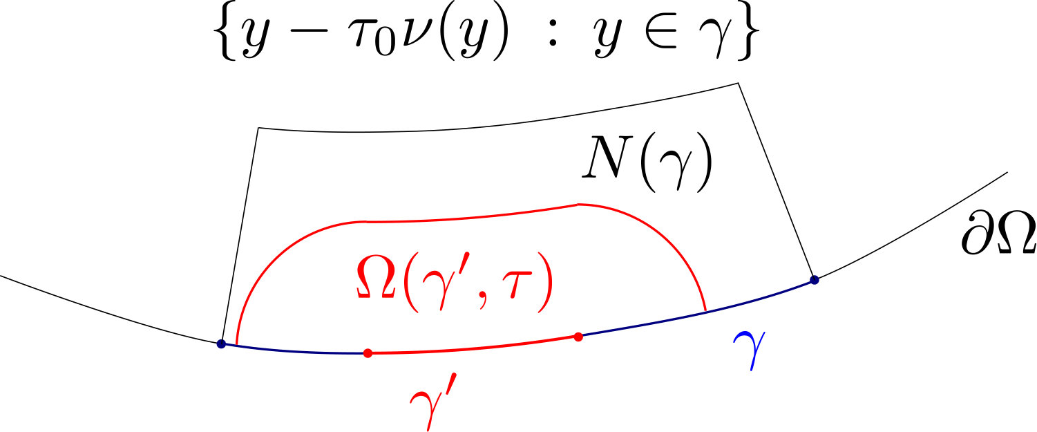 Figure 1
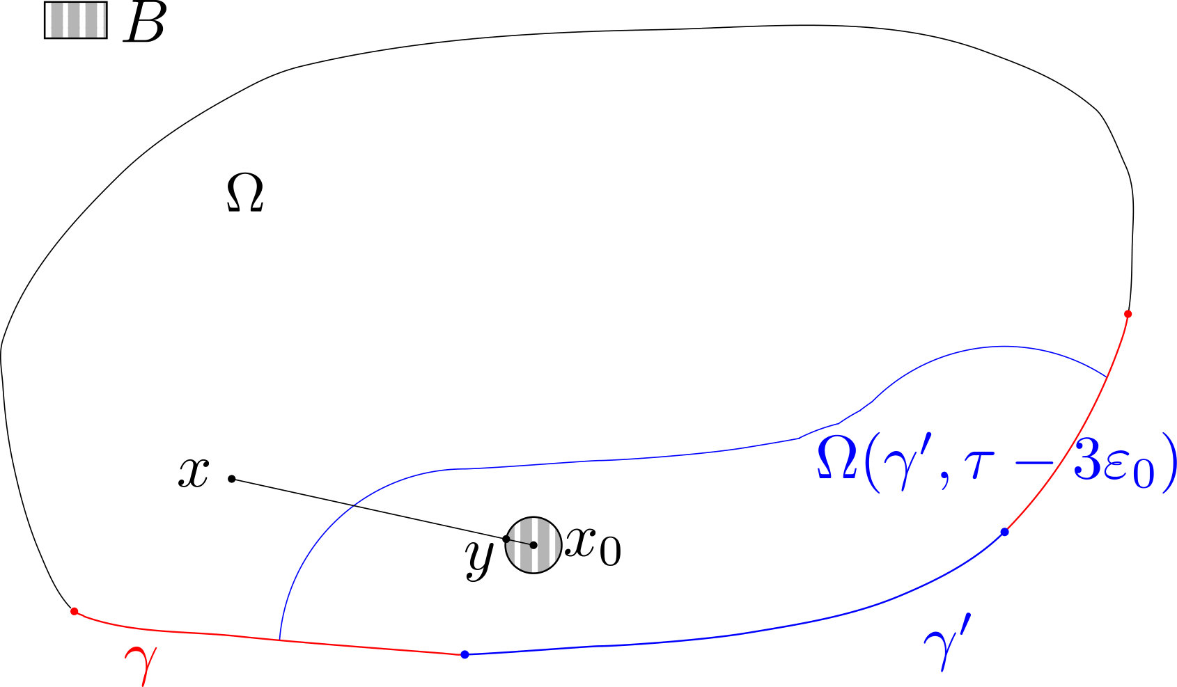 Figure 2
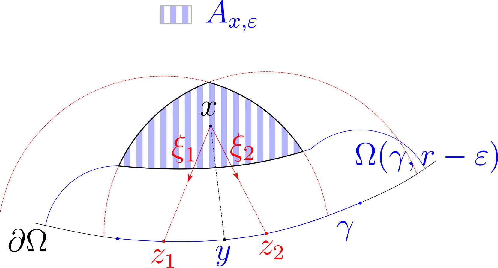 Figure 3
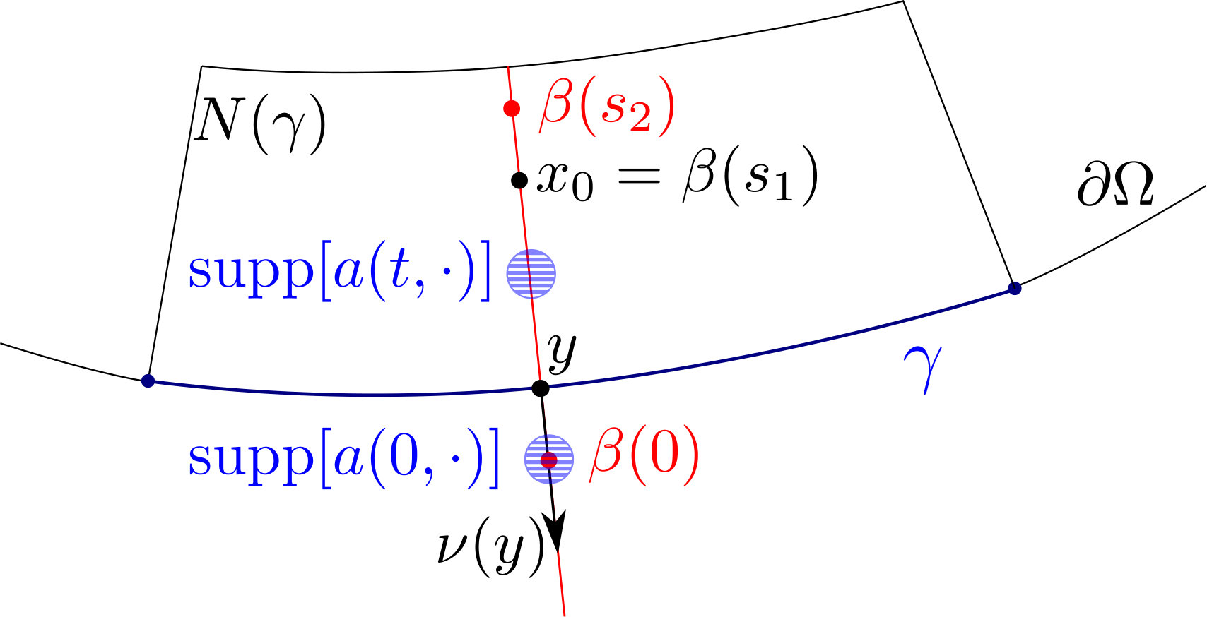 Figure 4
Peer Reviews
No public reviews on file for this paper yet. If you reviewed it on a platform where reviews are public (OpenReview, ICLR, NeurIPS, ICML), you can paste yours below so the community can read it here.
Videos
No videos yet. Explain this paper in a talk, walkthrough, or lecture? Add one.
Taxonomy
TopicsNumerical methods in inverse problems · Advanced Mathematical Modeling in Engineering · Composite Material Mechanics
Application of the boundary control method to partial data Borg-Levinson inverse spectral problem
Y. Kian1
1Aix Marseille Univ, Université de Toulon, CNRS, CPT, Marseille, France
,
M. Morancey2
2Aix Marseille Univ, CNRS, Centrale Marseille, I2M, Marseille, France
and
L. Oksanen3
3Department of Mathematics, University College London, London, UK
Abstract.
We consider the multidimensional Borg-Levinson problem of determining a potential , appearing in the Dirichlet realization of the Schrödinger operator on a bounded domain , , from the boundary spectral data of on an arbitrary portion of . More precisely, for an open and non-empty subset of , we consider the boundary spectral data on given by , where is the non-decreasing sequence of eigenvalues of , an associated Hilbertian basis of eigenfunctions, and is the unit outward normal vector to . We prove that the data uniquely determine a bounded potential . Previous uniqueness results, with arbitrarily small , assume that is smooth. Our approach is based on the Boundary Control method, and we give a self-contained presentation of the method, focusing on the analytic rather than geometric aspects of the method.
Keywords: Inverse problems, inverse spectral problem, wave equation, Boundary Control method, uniqueness, partial data, unique continuation.
Mathematics subject classification 2010 : 35R30, 35J10, 35L05.
1. Introduction
1.1. Statement of the results
We fix a bounded and connected domain of , , and a non empty open set of . We consider the Schrödinger operator acting on with Dirichlet boundary condition and real valued. The spectrum of consists of a non decreasing sequence of eigenvalues , with , to which we associate a Hilbertian basis of eigenfunctions . Then, we introduce the boundary spectral data restricted to the portion given by
[TABLE]
with the outward unit normal vector to and the normal derivative. The main goal of the present paper is to prove uniqueness in the recovery of from the data .
Theorem 1.1**.**
Assume that is convex, is open and non empty, and , . Then implies .
This result will be proved by applying the so called Boundary Control method that we adapt to the present setting with a convex domain and a bounded potential.
Let us also formulate a dynamic variant of Theorem 1.1. Fix , with , and consider the initial boundary value problem (IBVP in short)
[TABLE]
According to [18, Theorem 2.1], for , the problem (1.1) admits a unique solution
[TABLE]
which satisfies . Thus we can define the partial Dirichlet-to-Neumann map
[TABLE]
We define also . The dynamic variant can be stated in the following way
Theorem 1.2**.**
Assume that is convex, is open and non empty, , and , . Then implies that .
1.2. Previous literature
Our problem is a generalization to the multidimensional case of the pioneering work of Borg [4], Levinson [21], Gel’fand and Levitan [7] stated in an interval of , also called Borg-Levinson inverse spectral problem. The first multidimensional formulation of this problem is given by Nachman, Sylvester and Uhlmann [24] who applied the result of [28] to prove that determines uniquely . Päivärinta and Serov [25] extended this result to , and Canuto and Kavian [5] to more general perturbations of the Laplacian. Isozaki [9] proved that the uniqueness still holds if finitely many eigenpairs remain unknown and [6, 12, 13] proved that only some asymptotic knowledge of is enough for the recovery of as well as more general coefficients.
Let us now turn to partial data results. For arbitrarily small , the known uniqueness results are based on the Boundary Control method introduced by Belishev [2]. In [10], under the assumption that is smooth, Katchalov and Kurylev proved that the data , with the exception of finitely many eigenpairs, determines , and [11] proved that the uniqueness remains true when knowing only the partial boundary spectral data , with an arbitrary portion of the boundary. The novelty of the present paper is to consider non-smooth .
Let us remark that more general operators than the Schrödinger operator have been considered. It was proved in [3] that, when is a smooth Riemanian manifold the boundary, the spectral data determines the Riemanian manifold up to an isometry. Moreover, arbitrary smooth and symmetric lower order perturbations of the Laplace-Beltrami operator can be determined up to natural gauge transformations, see [15] and, for the case of equations taking values on Hermitian vector bundles, [17]. These results allow to be arbitrarily small. It is an open question, however, if the recovery of non-symmetric lower order perturbations is possible without further geometric assumptions. The known results [16] assume that satisfies the geometric control condition [1].
All the results of the present paper can be extended to the recovery of more general coefficients on a smooth Riemannian manifold, by changing some intermediate tools and by replacing the last part of the proof, that is, the global recovery step, with the iterative process described in [17, Section 4.2]. The assumption of convexity allows us to simplify in various way the exposition in order to emphasize the main idea, and analytic aspects, of the Boundary Control method. The geometric aspects are mostly avoided, since for a pair points on a convex domain, the shortest path between the points is simply a line segment. For these reasons the present paper can also be considered as an introduction to the Boundary Control method.
The dynamic variant in Theorem 1.2 allows for a more fine grained notion partial data where is supported on a part of boundary, disjoint from the part on which is restricted. Such disjoint data questions have been studied in [19, 20], however, the techniques used the present paper do not readily extend to disjoint data cases.
1.3. Outline
In Section 2 we recall some properties of solutions of (1.1) that will be used in the proof of Theorem 1.1. In Section 3 we describe the Boundary Control method and use it to show that can be recovered locally near . Building on the local recovery step, we show in Section 4 the global recovery as stated in Theorem 1.1. In Section 5 we show how to prove Theorem 1.2 by adapting the proof of Theorem 1.1. For the convenience of the reader, we prove in the appendix some well-known facts formulated in Section 2.
2. Finite speed of propagation and unique continuation
The Boundary Control method is based on two complementary properties of the wave equation (1.1): the finite speed of propagation and unique continuation. Loosely speaking, they give respectively the maximum and minimum speeds at which waves can propagate. It is essential for the Boundary Control method that these two speeds are the same in the case of a scalar valued wave equations such as (1.1). All the results recalled in this section are well-known, however, for the convenience of the reader, we give their proofs in the appendix.
2.1. Finite speed of propagation and domains of influence
We make the standing assumption that is convex and define
[TABLE]
We write also , , . A typical formulation of the finite speed of propagation is as follows
Lemma 2.1**.**
Let , let , and let . Define the cone
[TABLE]
and consider satisfying in . Then
[TABLE]
imply .
A proof of this classical result can be found e.g. in [11, Theorem 2.47]. Let us now reformulate Lemma 2.1 by using the notion of domain of influence.
Definition 2.1**.**
For every and every open subset of we define the subset of given by
[TABLE]
The set is called the domain of influence of at time .
Theorem 2.1**.**
Let be an open subset of and . Let solve (1.1) with satisfying . Then .
We give a proof of this theorem in the appendix. The proof is a short reduction to Lemma 2.1.
2.2. Unique continuation and approximate controllability
The local unique continuation result [29] by Tataru implies the following global Holmgren-John type unique continuation
Theorem 2.2**.**
Let , let be an open subset of , and let . Consider
[TABLE]
satisfying in . Then
[TABLE]
implies , .
We give a proof of this theorem and the following corollary in the appendix. The corollary is often called approximate controllability. We denote by the solution of (1.1) when emphasizing the dependence on the boundary source .
Corollary 2.1**.**
Let be an open subset of and . Then the set
[TABLE]
is dense in .
Here is considered as the subspace of consisting of functions vanishing outside . Note that Theorem 2.1 implies that the set (2.2) is indeed contained in the subspace , and in this sense, Corollary 2.1 relates the finite speed of propagation and unique continuation. The Boundary Control method depends heavily on this relation, as described in the next section.
3. Local recovery of the potential
We make the following standing assumption
- (A)
is convex, is open and non-empty, and , ,
and write . In this section we prove the following
Theorem 3.1**.**
Suppose that . Then there are and a non-empty open set such that
[TABLE]
3.1. From boundary spectral data to inner products of solutions
We write for the solution of (1.1) with , , and . Moreover, we denote by , , a fixed Hilbertian basis of eigenfunctions of , . Let us begin by showing that the Fourier coefficients of , with respect to the bases , , coincide for and .
Lemma 3.1**.**
Suppose that . Let satisfy . Then
[TABLE]
Proof.
Write , . We start by assuming that . Then . Setting and integrating by parts we find
[TABLE]
As , we deduce that both , , solve the same differential equation
[TABLE]
which implies (3.2). By density, (3.2) holds also for satisfying .
∎
Under the assumptions of Lemma 3.1, it holds in particular that
[TABLE]
where is the solution of (3.3).
3.2. Inner products on domains of influence
We denote by the indicator function of a set , that is, if and otherwise. Let us show that (3.5) holds when is replaced by a domain of influence in the following sense
Lemma 3.2**.**
Suppose that . Let supported in , let be open, and let . Then
[TABLE]
Proof.
By Corollary 2.1, there is a sequence in such that converges to in as . As is the orthogonal projection of into the subspace , it holds, using again the density in Corollary 2.1, that
[TABLE]
Now (3.5) implies that
[TABLE]
and also that for any
[TABLE]
The last two equalities imply
[TABLE]
The convergence of and (3.4) imply that is a Cauchy sequence, and therefore it converges. Corollary 2.1 and (3.6) imply that converges to . Finally, by (3.5),
[TABLE]
∎
From this result, we deduce the following corollary.
Corollary 3.1**.**
Suppose that . Let be supported in , and let and . Then
[TABLE]
Proof.
For , we fix
[TABLE]
For , since , by the Sobolev embedding theorem for
[TABLE]
we have . Thus, an application of the Hölder inequality yields
[TABLE]
Thus, for , we have
[TABLE]
On the other hand, Lemma 3.2 implies
[TABLE]
Combining this with (3.8) and sending , we deduce (3.7).
∎
The proof of Lemma 3.2 can be iterated as follows.
Lemma 3.3**.**
Suppose that . Let be supported in , let be open, and let . Then
[TABLE]
Proof.
By the proof of Lemma 3.2, there is a sequence in such that for both and , the functions converge to in as . Then by Lemma 3.2,
[TABLE]
∎
3.3. Recovery of internal data near
Let and let be one of the closest point in to . Then the line through and must intersect perpendicularly. Conversely, a point is the closest point in to for small . Here is the outward unit normal vector at . Furthermore, there is such that
[TABLE]
We will show that Theorem 3.1 holds with any choice of and satisfying
[TABLE]
This hypothesis as well as the set introduced in the following lemma are illustrated in Fig. 1.
We show next that inner products on domains of influence can be used to determine the following pointwise products
Lemma 3.4**.**
Suppose that . Let be supported in . Then
[TABLE]
where .
Proof.
To illustrate the idea of the proof, let us suppose for a moment that , , and are smooth. Then for smooth and , also the functions and are smooth. Let , , and set , , . Then as . By taking a limit analogous to that in Corollary 3.1, it follows from Lemma 3.3 that
[TABLE]
where and . Combining this with Corollary 3.1, we obtain
[TABLE]
and therefore, denoting the volume of by ,
[TABLE]
Letting , we obtain .
Let us now turn to the case of bounded , . The above argument does not generalize immediately, since the limit with respect to might not exist in the non-smooth case. Our remedy is to replace the sets with sets of bounded eccentricity.
Let be as above. Choose unit vectors , that form a basis of , and that are small enough perturbations of so that the lines intersect in near . Denote the points of intersection by , and consider the sets
[TABLE]
The construction of the set is illustrated in Fig. 2.
For small , the set is approximated in the first order by the simplex with outward normals and , , and all the faces having distance to . Thus is of bounded eccentricity and as .
By repeating the proofs of Lemma 3.3 and Corollary 3.1 several times, we obtain analogously to the smooth case,
[TABLE]
The Lebesgue differentiation theorem, see e.g. [27, Chapter 7, Theorem 7.14], implies the claim. Note that the products in the claim are interpreted as -functions.
∎
Lemma 3.5**.**
Suppose that . Let be supported in . Then
[TABLE]
Proof.
We will choose in Lemma 3.4 to be a suitable geometric optics solution, and begin by constructing such solutions. Let , , and set . Let be small and set and . The line satisfies , , and . Hence if is small enough and has small enough support, then the function satisfies
[TABLE]
In particular, . The support of this particular solution is illustrated in Fig. 3.
To simplify the notation, we suppose that is real valued, and write . Then we consider
[TABLE]
where solves
[TABLE]
It follows that in and, analogously to [14, Lemma 2.2] one can check that
[TABLE]
Moreover, (3.11) implies that
[TABLE]
Define , , . Then (3.11) implies that .
We have on . Up to a reduction of we can assume that for , thus on . Therefore Lemma 3.4 implies that for all , , , , and ,
[TABLE]
Integrating both sides of this expression and sending , we get
[TABLE]
After the change of variables ,
[TABLE]
As and are arbitrary cutoff functions with small supports, it holds that for and near . As can be taken arbitrarily small and can be chosen arbitrarily, the claim follows.
∎
3.4. Proof of Theorem 3.1
Choose and open and non-empty satisfying (3.9). Lemmas 3.1, 3.5 and the finite speed of propagation imply that for any ,
[TABLE]
This together with Corollary 2.1 implies that in . Thus in it holds that
[TABLE]
Integrating this expression on we get , . This proves (3.1).∎
4. Global recovery
The goal of this section is to get global recovery of the potential from the local determination. More precisely, we will complete the proof of Theorem 1.1. We start by fixing the notation. From now on we consider and such that condition (3.1) is fulfilled and we assume that . For any open connected set of we define the operator
[TABLE]
Moreover, for , we define
[TABLE]
with solving
[TABLE]
We write also
[TABLE]
Lemma 4.1**.**
Fix and consider for the set . Then, we have
[TABLE]
Moreover, if we have
[TABLE]
Proof.
The equation (4.2) follows immediately from Lemma 3.5. Let and set . Then integrating by parts, we find
[TABLE]
Then (4.2) implies
[TABLE]
As is arbitrary we deduce that on . Thus, fixing and using (3.1), we deduce that on , . In particular, for any , we have on , . Thus, the unique continuation property of Theorem 2.2 implies that, for any , we have on . On the other hand, using the fact that
[TABLE]
one can check that the restriction of to solves the problem
[TABLE]
which implies that , . Combining these two identities we deduce (4.3).
∎
We extend the notion of domain of influence for any and any open set by setting
[TABLE]
From now on, we fix , , dist, . Note that . In the remaining of this text we will prove that (4.3) implies that in . Note first that according to the finite speed of propagation we have
[TABLE]
This is the analogue of Theorem 2.1 for solutions of (4.1).
We will also need to use global unique continuation in the domain . In the appendix, we discuss unique continuation only under assumptions that allow us to avoid certain arguments of geometric nature. For this purpose let be a domain with smooth boundary. We fix an open subset of and for every , we consider the set . Then, we introduce the following condition on :
(H) Let . If then . Furthermore, if then for every neighborhood of in there exists such that .
As is convex, this condition holds for any . Now, let us recall (as illustrated in Fig. 4) that for any , is the unique element of satisfying dist. Moreover, since is convex we have and can not meet since is the unique element of satisfying dist. Therefore, we have and satisfies condition (H). Theorem 2.2 with replaced by and implies the following analogue of Corollary 2.1.
Lemma 4.2**.**
For , the set
[TABLE]
is dense in .
For convenience of the reader, we have included a proof of this lemma in the appendix. The proof is analogous with the proof of Corollary 2.1. Let us also show that the norm of solution of (4.1) with is determined by condition
[TABLE]
which follows from (4.3) and the fact that . We have the following analogue of (3.5)
Lemma 4.3**.**
Condition (4.6) implies that, for all and all , we have
[TABLE]
Proof.
Consider for and for all the function . Integrating by parts, for all , we find
[TABLE]
Then, applying (4.6), we deduce that, for all , we have
[TABLE]
Moreover, for , we have . Thus, applying (4.8), we deduce that solves the system associated with the wave equation
[TABLE]
From unique continuation we can deduce that
[TABLE]
Therefore, solves
[TABLE]
Then, the uniqueness of this initial boundary value problem implies that which, according to the continuity of with respect to , implies that for all we have . This proves (4.7).
∎
Proof of Theorem 1.1.
In a similar way as in the previous section, for any , , we consider the unique element of such that dist. One can check that there exist such that is a basis of . Moreover, we can choose such that for
[TABLE]
the family is of bounded eccentricity and
[TABLE]
Combining the density of the set (4.7) with the arguments used in Lemma 3.4, we obtain
[TABLE]
for all . After taking the limit , we obtain
[TABLE]
From now on our goal will be to use this identity to conclude. For this purpose, in a similar way to Theorem 3.1 we will use special solutions that we will introduce next in order to recover for any . Then we will complete the proof. Let us first fix and consider dist. Since we know that . Now consider
[TABLE]
We fix also
[TABLE]
and we consider . Note that according to the definition of we have . Now let , and define
[TABLE]
Then, we consider,
[TABLE]
where solves
[TABLE]
It follows that in and one can check that
[TABLE]
with independent of . Then, we consider satisfying for and for . Then, we introduce
[TABLE]
It is clear that
[TABLE]
Moreover, in view of (4.12), we know that
[TABLE]
Using the fact that
[TABLE]
we deduce that
[TABLE]
Combining this with, (4.14) we deduce that
[TABLE]
In the same way, (4.14) implies that
[TABLE]
and fixing , we deduce that . Now let us show that with supp. For this purpose note first that
[TABLE]
On the other hand, we have
[TABLE]
and we deduce that
[TABLE]
Thus, condition (3.1) implies that, for all , we get
[TABLE]
Moreover, condition (4.4) implies
[TABLE]
and, in virtue of (3.1), we deduce that
[TABLE]
Combining this with (4.12), we deduce that the restriction of , , to solves
[TABLE]
The uniqueness of solutions for this IBVP implies that
[TABLE]
Combining this with (4.16), we deduce that and (4.17) implies that supp. Applying (4.11), one can check that, for all and , we have
[TABLE]
Integrating both sides of this expression, we get
[TABLE]
Then, in view of (4.13), sending and using the fact that on , we get
[TABLE]
Consider and fix . Note that supp and (4.15) implies that, for all , supp. Thus, (4.18) becomes
[TABLE]
Making the substitution , we obtain
[TABLE]
and making the substitution , we find
[TABLE]
Allowing , to be arbitrary, we deduce that for almost every we have
[TABLE]
which, by fixing , implies that
[TABLE]
Then, using the fact that , we deduce that
[TABLE]
Sending , we prove that
[TABLE]
Now allowing to be arbitrary we deduce that
[TABLE]
Then, (4.6) implies
[TABLE]
and we get
[TABLE]
Using this identity we will complete the proof of the theorem. For this purpose, note first that repeating the arguments of Lemma 3.1 one can check that
[TABLE]
Then, (4.19) implies that
[TABLE]
and the density results of Lemma 4.2 implies
[TABLE]
Combining this with arguments similar to the end of the proof of Theorem 3.1 we deduce that .
∎
5. Recovery from the Dirichlet-to-Neumann map
This section is devoted to proof of Theorem 1.2. The proof of this result is similar to the one of Theorem 1.1 and the boundary spectral data can be replaced by the Dirichlet-to-Neumann map as far as . The only point that we need to check is the following.
Lemma 5.1**.**
Let . For satisfy , supp and, for , we fix be the solution of (1.1) with . Condition implies that, for all and all , we have
[TABLE]
The proof is similar with that of Lemma 4.3, however, we give it for the convenience of the reader.
Proof.
Consider for and for all the function . Then, integrating by parts, we find
[TABLE]
Moreover, for , we have . Thus, applying (4.6), we deduce that solves the system associated with the wave equation
[TABLE]
Repeating the argument developed in the proof of Lemma 4.3 leads to . This proves (5.1).
∎
Using (5.1) and repeating the arguments used for Theorem 3.1, we can show that
[TABLE]
for some and . Fixing , we consider the following
Lemma 5.2**.**
Let satisfy (3.1). Then the condition implies that
[TABLE]
Moreover, we get
[TABLE]
Proof.
Note first that according to (3.1), satisfies on and the condition implies . Thus, from the unique continuation property of Theorem 2.2 we deduce (5.2). In view of (5.2), we deduce (5.3) by mimicking the proof of statement (4.3) in Lemma 4.1 .∎
Armed with this lemma and the arguments used for the global recovery in Section 4 we can complete the proof of Theorem 1.2.
Appendix A Proofs of classical results on wave equations
We begin by proving the reformulation of the finite speed of progation as stated in Section 2.1.
Proof of Theorem 2.1.
Let . Then we have dist. Fixing , and applying Lemma 2.1, we obtain . For and any , we obtain that
[TABLE]
which implies that . Thus, on a neighborhood of and . This completes the proof of Theorem 2.1.
∎
Let us now turn to the unique continuation result formulated in Section 2.2. Recall that Theorem 2.2 follows from a local Holmgren-John unique continuation. Consider a smooth surface . We say that the differential operator is non-characteristic at a point if the outward unit normal vector with respect to at , with , , satisfies . For all and all , we fix
[TABLE]
Theorem A.1**.**
Let . Assume that there exists such that and such that is non-characteristic at . Then, if solves in and satisfies then .
This theorem is a special case of [29, Theorem 1] (see also [26] for related results). We refer also to [11, Theorem 2.66] for a proof without microlocal analysis. In order to prove Theorem 2.2, we fix and we consider two intermediate results.
Lemma A.1**.**
Let , and . Assume that there exists solving in and satisfying
[TABLE]
Then, we have
[TABLE]
with
[TABLE]
Proof.
We start by introducing the set
[TABLE]
and we remark that and . The surface are smooth with the exception of the end points . In addition, for , the points are non-characteristic with respect to .
Indeed, for every the normal derivative (modulo multiplication by ) of is given by
[TABLE]
and we clearly have
[TABLE]
This proves that, for , is non-characteristic at any . We fix
[TABLE]
Let us show ad absurdio that . For this purpose let us assume that . According to (A.1), we have and it is clear that for any such that
[TABLE]
there exists such that . Then, the definition of implies that on a neighborhood of .
According to the local unique continuation result of Theorem A.1, since is non-characteristic and since , we deduce that on a neighborhood of every point of . Moreover, if we have and (A.1) implies that on a neighborhood of . Thus, there is an open neighborhood of such that . As is compact, there exists such that . This contradicts the definition of and we deduce that . This completes the proof of the lemma.
∎
From the previous result we can deduce the following.
Lemma A.2**.**
Let be an open set of and let . Consider and , such that
[TABLE]
Let be a solution of in satisfying
[TABLE]
Then, we have
[TABLE]
with
[TABLE]
Proof.
Without loss of generality we assume that . Then our goal is to show that for any and any such that we have . We divide this proof into two steps.
First step: let and consider defined by
[TABLE]
We have and is a solution of in . Moreover, since , fixing and , (A.4) implies that on . Therefore, applying Lemma A.1 to , we deduce that
[TABLE]
In particular we have
[TABLE]
This shows that
[TABLE]
Second step: let and consider defined by
[TABLE]
Then, for any and applying again Lemma A.1, we deduce that
[TABLE]
In particular, we have
[TABLE]
Since is arbitrary, we can send and deduce that
[TABLE]
Therefore, we have
[TABLE]
Finally, combining (A.6)-(A.7), we deduce (A.5).
∎
We are now in the position to complete the proof of Theorem 2.2.
Proof of Theorem 2.2 under the assumption (H).
Replacing by , we can without loss of generality assume that on and on . Then, fixing the cone
[TABLE]
the proof will be completed if we show that
[TABLE]
Here we use the fact that .
Fix such that . We consider arbitrary small. Then, according to condition (H), there exists such that , and . We define and we clearly have . By eventually reducing the size of , we can assume that the element given by
[TABLE]
is lying in and . Moreover, fixing , which can be arbitrary small since can be arbitrary small, we deduce that . We extend by [math] to . Since on , we deduce that . Therefore extending to we deduce that solves in . Using the fact that , we consider the path
[TABLE]
which is lying in . Since is compact there exists such that dist and dist. Now let be such that . Here we can eventually reduce the size of in order to have . Choose , such that , , and denote . We can now apply Lemma A.2 to complete the proof of the theorem. Indeed, we can choose , which can be arbitrary small, such that on . Hence, Lemma A.2 implies that in
[TABLE]
On the other hand, using the fact that , for all , we have
[TABLE]
Therefore, using the fact that , we find
[TABLE]
and
[TABLE]
Repeating this process and by eventually reducing the size of , we find
[TABLE]
Note that here we use the fact that
[TABLE]
Using the fact that , we get
[TABLE]
Therefore, using the fact that dist and the fact that and are arbitrary and is independent of , we can choose and in such a way that dist. It follows that
[TABLE]
and we have
[TABLE]
This proves (A.8) and Theorem 2.2. ∎
The rest of the appendix concerns the proofs of the two approximate controllability results that we need.
Proof of Corollary 2.1.
In order to prove the density result we fix , extended by zero to , such that
[TABLE]
and we will prove that . For this purpose, let solves
[TABLE]
In light of [18, ,Theorem 2.1], we have . Thus, for all , integrating by parts and applying (1.1) and (A.9), we find
[TABLE]
Allowing be arbitrary we deduce that . Now fixing defined by
[TABLE]
we deduce that satisfies
[TABLE]
Thus, in view of Theorem 2.2, we have . This proves the density of (2.2).
∎
Proof of Lemma 4.2.
In order to prove the density result we fix , extended by zero to , such that
[TABLE]
and we will prove that . For this purpose, let solves
[TABLE]
Then, for all , integrating by parts and applying (A.11), we find
[TABLE]
Allowing be arbitrary we deduce that . Now fixing defined by
[TABLE]
we deduce that satisfies
[TABLE]
Thus, in view of the proof of Theorem 2.2, we have . This proves the density of (4.5).
∎
The reference list from the paper itself. Each links out to its DOI / PubMed record.
- 1[1] C. Bardos, G. Lebeau, J. Rauch, Sharp sufficient conditions for the observation, control, and stabilization of waves from the boundary , SIAM Journal on Control and Optimization, 30 no. 5 (1992), 1024-1065.
- 2[2] M. Belishev , An approach to multidimensional inverse problems for the wave equation , Dokl. Akad. Nauk SSSR, 297 (1987), 524-527.
- 3[3] M. Belishev and Y. Kurylev , To the reconstruction of a Riemannian manifold via its spectral data (BC-method) , Comm. Partial Differential Equations, 17 (1992), 767-804.
- 4[4] G. Borg , Eine Umkehrung der Sturm-Liouvilleschen Eigenwertaufgabe , Acta Math., 78 (1946), 1-96.
- 5[5] B. Canuto and O. Kavian , Determining Two Coefficients in Elliptic Operators via Boundary Spectral Data: a Uniqueness Result , Bolletino Unione Mat. Ital. Sez. B Artic. Ric. Mat. (8), 7 no. 1 (2004), 207-230.
- 6[6] M. Choulli and P. Stefanov , Stability for the multi-dimensional Borg-Levinson theorem with partial spectral data , Commun. Partial Diff. Eqns., 38 (3) (2013), 455-476.
- 7[7] I. M. Gel’fand and B. M. Levitan , On the determination of a differential equation from its spectral function , Izv. Akad. Nauk USSR, Ser. Mat., 15 (1951), 309-360.
- 8[8] L. Hörmander , Linear partial differential operators , Springer Verlag, Berlin-New York, 1976.