Hidden sector behind the CKM matrix
Shohei Okawa, Yuji Omura

TL;DR
This paper proposes a hidden sector model where new particles at the TeV scale mediate quark flavor violation, explaining the CKM matrix and providing a dark matter candidate with specific properties and detectable signals.
Contribution
It introduces a simple scenario linking the CKM matrix to a hidden sector that also contains a dark matter candidate, with explicit predictions for DM mass and couplings.
Findings
Dark matter mass around the TeV scale
Yukawa couplings between DM and quarks are between 0.01 and 1
Predicted spin-independent DM cross section is about 10^{-9} pb
Abstract
The small quark mixing, described by the Cabibbo-Kobayashi-Maskawa (CKM) matrix in the Standard Model, may be a clue to reveal new physics around the TeV scale. We consider a simple scenario that extra particles in a hidden sector radiatively mediate the flavor violation to the quark sector around the TeV scale and effectively realize the observed CKM matrix. The lightest particle in the hidden sector, whose contribution to the CKM matrix is expected to be dominant, is a good dark matter (DM) candidate, so we focus on the contribution, and discuss the DM physics. In this scenario, there is an explicit relation between the CKM matrix and flavor violating couplings, such as four-quark couplings, because both are radiatively induced by the particles in the hidden sector. Then, we can explicitly find the DM mass region and the size of Yukawa couplings between the DM and quarks, based on the…
Click any figure to enlarge with its caption.
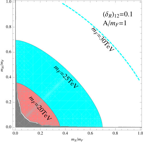 Figure 1
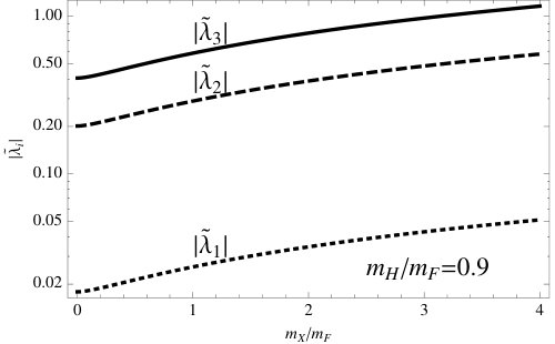 Figure 2
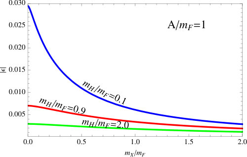 Figure 3
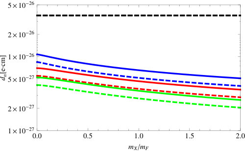 Figure 4
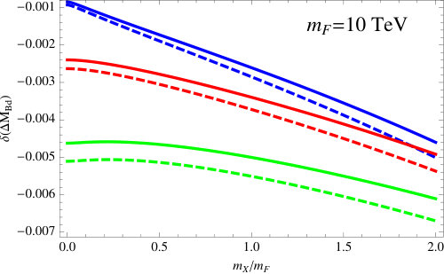 Figure 5
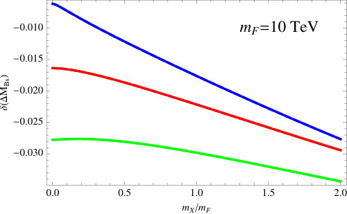 Figure 6
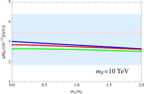 Figure 7
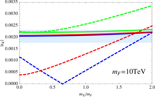 Figure 8
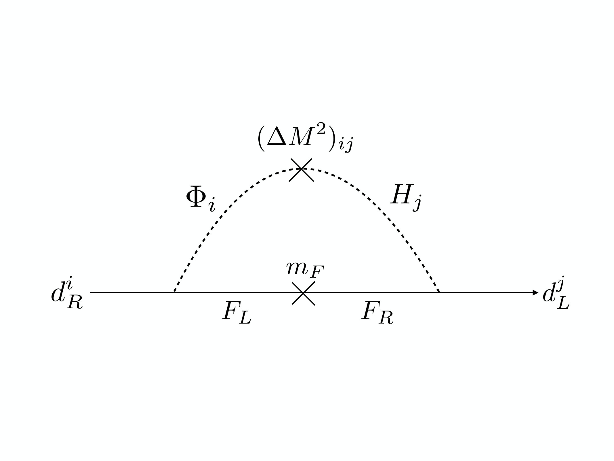 Figure 9
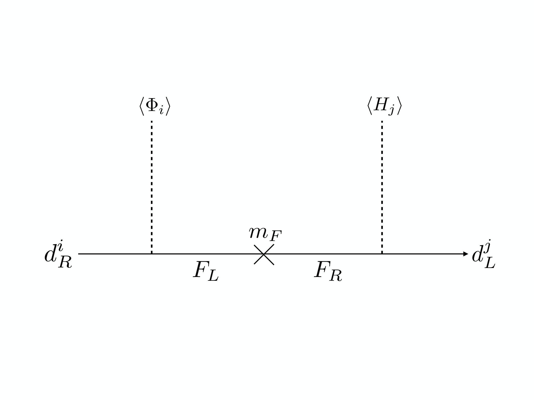 Figure 10
| Fields | spin | flavor charge | |||
|---|---|---|---|---|---|
| 1/2 | |||||
| 1/2 | |||||
| 1/2 | |||||
| 0 |
| Fields | spin | Dark charge | |||
| 1/2 | |||||
| 0 | |||||
| 0 |
Peer Reviews
No public reviews on file for this paper yet. If you reviewed it on a platform where reviews are public (OpenReview, ICLR, NeurIPS, ICML), you can paste yours below so the community can read it here.
Videos
No videos yet. Explain this paper in a talk, walkthrough, or lecture? Add one.
**Hidden sector behind the CKM matrix
**
Shohei Okawa1 and Yuji Omura2
1* Department of Physics, Nagoya University, Nagoya 464-8602, Japan
2* Kobayashi-Maskawa Institute for the Origin of Particles and the Universe,
Nagoya University, Nagoya 464-8602, Japan
The small quark mixing, described by the Cabibbo-Kobayashi-Maskawa (CKM) matrix in the Standard Model, may be a clue to reveal new physics around the TeV scale. We consider a simple scenario that extra particles in a hidden sector radiatively mediate the flavor violation to the quark sector around the TeV scale and effectively realize the observed CKM matrix. The lightest particle in the hidden sector, whose contribution to the CKM matrix is expected to be dominant, is a good dark matter (DM) candidate. There are many possible setups to describe this scenario, so that we investigate some universal predictions of this kind of model, focusing on the contribution of DM to the quark mixing and flavor physics. In this scenario, there is an explicit relation between the CKM matrix and flavor violating couplings, such as four-quark couplings, because both are radiatively induced by the particles in the hidden sector. Then, we can explicitly find the DM mass region and the size of Yukawa couplings between the DM and quarks, based on the study of flavor physics and DM physics. In conclusion, we show that DM mass in our scenario is around the TeV scale, and the Yukawa couplings are between and . The spin-independent DM scattering cross section is estimated as [pb]. An extra colored particle is also predicted at the TeV scale.
1 Introduction
The flavor structure of the Standard Model (SM) is one of mysteries, which are expected to be solved by extending the SM. In the SM, there are three generations in both quark and lepton sectors, and the difference among the generations is the size of the fermion masses. The fermion masses are dynamically generated by the spontaneous electroweak (EW) symmetry breaking, and the observed masses and mixing are given by the Yukawa couplings with the Higgs field in the SM. We know that the Yukawa couplings have to realize the large mass hierarchies and the small quark mixing. This unique form of the Yukawa matrix may be a clue to reveal the new physics above the EW scale.
If the Yukawa couplings are ignored in the SM Lagrangian, the flavor symmetry to rotate generations and phases of quarks is restored. Of these, the rotation symmetry of the generations is broken by quark mass terms; on the other hand, the symmetry to rotate the quark phases is respected even in the mass terms. The phase rotation is explicitly broken only by the Cabibbo-Kobayashi-Maskawa (CKM) matrix in the weak interaction. According to the experimental results, the CKM matrix is close to the identity matrix but has small mixing angles. These small mixing angles may imply that the flavor symmetry, especially to rotate the quark phases, is respected at high energy. If this is the case, new physics exists above the EW scale in order to break the flavor symmetry spontaneously and generate the realistic quark mixing. This simple scenario, however, possibly suffers from constraints from flavor violating processes. If the flavor symmetry breaking of the Yukawa couplings is generated at the tree level, large flavor changing neutral currents (FCNCs) are generally induced and the model is easily excluded. Therefore, we need consider a scenario that some new particles mediate the flavor symmetry breaking to the quark sector at a loop level.
We have another strong motivation to desire new physics above the EW scale, that is, the results of the cosmological observations proposed by the WMAP and Planck collaborations [1, 2]. They suggest that dark energy and dark matter (DM) dominate our universe and the amount of DM is about five times bigger than the visible particles. There are a lot possibilities for DM and one possible DM candidate is a Weakly-Interacting Massive Particle (WIMP) which resides around TeV scale. Then, we can expect that there is a direct connection between DM and the origin of the quark matrix.
Motivated by those mysteries, in this paper, we consider a simple scenario that extra particles, including DM, radiatively mediate the flavor symmetry breaking to the quark sector around the TeV scale and effectively realize the observed quark mixing. In our scenario, the flavor symmetry to rotate the quark phases in each generation is conserved at high energy in both of the up-type and down-type quark sectors. At the TeV scale, the flavor symmetry breaks down in a hidden sector. We also introduce an extra heavy quark and scalars charged under the flavor symmetry to mediate the flavor symmetry breaking to the quark sector. The mediators have flavor symmetric Yukawa couplings with only down-type quarks, but the fields to break the flavor symmetry do not couple to any SM fermions directly. The scalar mediators are only the fields to couple with the symmetry breaking fields, and then radiatively mediate the flavor symmetry breaking to the quark sector. We do not construct any explicit model for the flavor symmetry breaking, assuming that the effect of the symmetry breaking appears in the mass matrix of the scalar mediators. The rough sketch of this idea is shown in Fig. 1. , and correspond to the SM-singlet, the EW charged scalars, and the extra heavy quark as the mediators. is the part of the mass matrix for the scalars and denotes the flavor symmetry breaking effect. Note that we can find many similar setups motivated by the origin of the quark mixing[3, 4, 5, 6, 7, 9, 8, 10, 11, 12, 13, 14, 15, 16, 17, 18, 19, 20, 21, 22, 23, 24, 26, 25, 27, 28]. In the present work, we consider a simple setup motivated by DM as well as the explanation of the quark mixing, and survey predictions of this kind of model. The results could be applied to many concrete models that radiatively induce the quark mixing.
The lightest neutral particle among the scalars, and , is a good DM candidate. The one-loop contribution to the down-type quark Yukawa couplings in Fig. 1 is probably dominated by the contribution of the diagram involving the DM, because of the relatively light mass. Then, we simply focus on the physics of the DM and estimate the size of the predicted quark mixing and quark masses. As mentioned above, there are many possible setups to describe this kind of scenario [3, 4, 5, 6, 7, 9, 8, 10, 11, 12, 13, 14, 15, 16, 17, 18, 19, 20, 21, 22, 23, 24, 26, 25, 27, 28]. We could find some universal predictions, according to this simple assumption that the observed CKM matrix is originated from the one-loop corrections involving the DM.
Interestingly, the one-loop correction is roughly estimated as when the coupling between DM and quarks is a little smaller than . It is close to the order of the strange quark mass divided by the vacuum expectation value (VEV) of the Higgs field. In order to realize the CKM matrix, the required correction to the down-type Yukawa matrix is also between and , so that the couplings between DM and quarks should be in the range between and , depending on the DM mass. Then, we need not worry about the triviality bound concerned with the divergence of couplings and we can predict a sizable interaction between DM and nuclei.
Another important prediction is a direct connection between the CKM matrix and flavor violating couplings, such as four-quark couplings. In this kind of setup, the CKM matrix and the flavor-violating couplings have the same source, so that sizable deviations from the SM values in the flavor violating processes are predicted. It is known that the processes and the electric dipole moment (EDM) give stringent bounds to new physics contributions, so that the flavor physics constrains the mass scale of the heavy quark and the extra scalars. In our work, we see that the non-vanishing CP phases in the Wilson coefficients of the and the EDM operators are unavoidable, and then we conclude that the extra quark mass should be not less than about 10 TeV. Taking into account the vacuum stability and the relic density of DM, the DM mass range is predicted to be between about 1 TeV and 10 TeV. We also find an explicit prediction of the spin-independent DM scattering cross section in Sec. 4: [pb]. Then, we conclude that our DM candidate can be tested by the future prospect of the XENON1T experiment [29].
In Sec. 2, we introduce our setup and explain the underlying theory of our scenario. Then, we discuss how to realize the observed Yukawa couplings in the SM. Since there are correlations between the predicted CKM matrix and the contributions to the flavor violating processes involving DM, we can explicitly derive the DM mass region. This study is given in Sec. 3. Based on the study in Sec. 3, we discuss the DM physics in Sec. 4. In the last section, we summarize our results and give a short comment on the other setup of the mediation and hidden sectors, motivated by the origin of the quark mass matrices.
2 Setup
We propose a scenario that the small quark mixing in the SM is originated from flavor symmetry breaking in a hidden sector. In our assumption, there is a flavor symmetry to rotate quark phases in each generation. The flavor symmetry is spontaneously broken by some fields in the hidden sector at some scale. The SM quarks do not directly couple with any fields to break the flavor symmetry, but there exist an extra quark and extra scalars to mediate the breaking effect to the quark sector. The fields to mediate the breaking effect do not contribute to the dynamics of the flavor symmetry breaking, but the masses and the mass eigenstates are affected by the symmetry breaking.
First, let us summarize the matter content of the quark sector. The fields in the flavor base are shown in Table 1. , , and () are the left-handed quarks, right-handed up-type and down-type quarks in the flavor base. We introduce a flavor symmetry to rotate the quark phases and assign a flavor charge () to each quark such that the flavor symmetry is conserved even in the Yukawa interaction with the Higgs doublet ():
[TABLE]
The Yukawa couplings, and , are in the diagonal forms, so that no quark flavor mixing appears at this level. Note that the flavor symmetry is not needed to be continuous symmetry, like U(1). It is not specified in our paper, assuming that the flavor symmetry is broken only in the hidden sector above the EW scale.
In the hidden sector there are extra fields to break the flavor symmetry and mediate the breaking effect. Let us introduce flavor-charged scalars, and , together with a flavor-singlet colored particle, . The SM charges of are the same as the ones of right-handed down-type quarks. and are SM-singlet complex scalar and SU(2)L doublets charged under the flavor symmetry, respectively. Then, we write down the flavor conserving Yukawa couplings between the extra fields and down-type quarks:
[TABLE]
Here, we simply assume that the flavor symmetry is broken by some fields in the hidden sector except for and , and the mass eigenstates of and are fixed by the scalar potential involving the fields to break the symmetry.***The flavor symmetry might be explicitly broken. We do not specify the structure of the hidden sector. In the case that the flavor symmetry is spontaneously broken in the hidden sector, we can easily construct a model introducing extra flavored SM-singlet fields, . The potential for the flavor symmetry breaking is, for instance, given by , and each develops non-vanishing VEV. Note that could be real scalars, depending on the flavor symmetry. Then, we rewrite the scalars in the flavor base with the mass eigenstates denoted by , , , and :
[TABLE]
Each of the coefficients is given by the mass matrix including in Fig. 1. All of the scalars radiatively contribute to the quark mixing through the Yukawa coupling in Eq. (2). The size of the contribution from each scalar would depend on the detail of models. In fact, we can consider many setups to realize the observed quark mass matrix radiatively in the framework of the Grand Unified Theory [3, 4, 5, 6], Left-Right symmetric models [7, 9, 8], supersymmetric models [10, 11, 12, 13, 14, 15, 16, 17, 18, 19, 20, 21], and flavor symmetric models [22, 23, 24, 26, 25, 27, 28]. Our main motivations are, however, to find the connection between DM and the quark mixing in the SM and to look for universal predictions of this kind of model. Therefore, we especially concentrate on the case that the light scalars dominantly contribute to the quark mixing, and the lightest scalar is a DM candidate. In particular, we focus on a minimal setup to realize the observed quark mass matrix; that is, there are only two kinds of light scalars, and , in our simplified model. Assuming that and are relatively lighter than the others, we can approximately simplify the Yukawa couplings as,
[TABLE]
We discuss the physics in our scenario, using these Yukawa couplings only: and . We will give some comments on the contributions of and . The charge assignment of the main fields for the mediation is summarized in Table 2. Note that dark charges are also assigned to , and , to distinguish them from the SM particles. Thanks to the dark charge, and/or the neutral component of can be stable and good dark matter candidates to dominate our universe.
The scalar fields couple with the SM Higgs field as well, and the couplings, in addition to , are
[TABLE]
Now, we expect that and do not develop non-vanishing VEVs because of the positive and . is a trilinear coupling, that is effectively induced after the flavor symmetry breaking. The term couples the SM Higgs and the mediators, so that plays an important role in generating the CKM matrix.
Note that the mass terms of and have a lower bound from the condition for the vacuum stability. If the trilinear coupling, , is too large compared to and , unstable directions would appear at the origin. Then, we find the following condition for the mass terms:
[TABLE]
where denotes the VEV of the Higgs field: .
2.1 Realization of the realistic Yukawa couplings
We discuss how the quark mixing is generated in our scenario. The Yukawa couplings at the tree-level are given by Eq. (1), so that they lead the diagonal mass matrices for up-type and down-type quarks after the EW symmetry breaking:
[TABLE]
In our scenario, the flavor symmetry is broken in the hidden sector, and , and decouple with the quark sector above the EW scale. Then, the small quark mixing is effectively generated via the Yukawa couplings in Eq. (4). According to the one-loop correction as shown in Fig. 1, we obtain the mass matrix for the down-type quarks in the form of
[TABLE]
where is the factor that comes from the one-loop correction:
[TABLE]
is given by
[TABLE]
, and are the masses of the fields, , and , respectively. , , and are expected to be around the flavor symmetry breaking scale. The origin of may be independent of the breaking scale. could be estimated as when , and are larger than . Fig. 2 shows vs. , assuming (blue), (red), (green) and . We see that is expected to be between and in the parameter region.
The required size of Yukawa couplings for the down-type quarks are less than , so that the size of the loop correction can be compatible with the required values for the down-type quark masses, as well as the CKM matrix. Note that and are complex parameters, in principle, so CP phases are also generated by this dynamics.
Now, we define the mass eigenstates and derive the relation between the realistic mass matrix and the extra Yukawa couplings: and . The Yukawa matrix for the up-type quarks is in the diagonal form in Eq. (7). Precisely speaking, there would be additional contributions from the wave function renormalization factor and the loop correction involving and . The former is suppressed by in the mass matrix and the later is assumed to be sub-dominant in our scenario.†††Fig. 2 shows that we could obtain at least 10 % suppressions compared to the contributions of and , if the masses of and are larger than . Then, we approximately derive the following relation, using the mass matrix in Eq. (8):
[TABLE]
denote the quark masses: . is the CKM matrix and is the diagonalizing matrix which rotates right-handed down-type quarks. Here, and are the three-dimensional vectors, and they correspond to the Yukawa couplings with DM (scalars) and in the mass base:
[TABLE]
where and are the mass eigenstates. We define and . In our notation, the mass eigenstates are . As we see in Sec. 3, the flavor violating couplings that contribute to the processes are also generated by the Yukawa couplings via the box diagram involving , and . According to the relation in Eq. (11), and are explicitly related to the CKM matrix and the quark masses, so that we can expect to obtain explicit predictions to the flavor violating processes. Before the detailed analyses of the flavor physics, let us discuss the consistency with the realistic Yukawa couplings and estimate the size of and lead by Eq. (11).
Assuming and using the relation of the diagonal elements in Eq. (11), can be approximately estimated as
[TABLE]
As discussed below, becomes the same order as , but is also required to be realistic.
Similarly, the off-diagonal elements of Eq. (11) lead the conditions for and . The assumption, , implies and each size is estimated as
[TABLE]
Assuming , the alignment of and are expected to be
[TABLE]
In our numerical study discussed below, we approximately evaluate and , assuming
[TABLE]
is fixed by the (2, 2) element of Eq. (11). The off-diagonal elements of Eq. (11) lead : to a good approximation,
[TABLE]
is from the CKM matrix: . Note that there is a prediction for and according to the mass matrix in Eq. (8):
[TABLE]
where is defined. need satisfy this condition and is assumed in our study. Note that in this parametrization is evaluated as
[TABLE]
This estimation is a good approximation to realize the observed Yukawa couplings. We expect that there are also some corrections from other extra particles, such as and , so we allow 10 % deviation in the down-type quark masses. In our analysis, we use the input parameters for the quark masses [30] and the CKM matrix [31] derived from the values in Table 3. When we compare our prediction with the realistic Yukawa couplings, we evaluate the quark masses at TeV, using the SM RG running at the two-loop level [32, 33].
Figure 3 shows the size of depending on , assuming that and . The CP phases and are fixed at and , respectively. It is interesting that this hierarchical Yukawa couplings, , have been proposed in Ref. [34], motivated by DM physics and flavor physics.
In Sec. 3, we discuss flavor physics in this setup and specify the DM mass region consistent with the experimental results. We see that , which appear in Eq. (11), directly relate to the flavor violating couplings which contribute to the processes. Therefore, we can explicitly derive the lower bound on the flavor symmetry breaking scale.
3 Flavor physics
In this section, we discuss flavor physics in our scenario. As well known, the processes, such as -, are the most sensitive to the new physics contributions. In addition, the CP-violation and the rare meson decay possibly constrain our model. First, we study the processes and discuss the deviations from the SM predictions, based on the result in Sec. 2. Then, we study the other observables: e.g., and the neutron EDM. In particular, we see that our model is strongly constrained by the CP-violation of the - mixing and the EDM.
3.1 processes
In our scenario, the CKM matrix is radiatively generated by , and in the hidden sector. In addition, the extra fields induce the operators relevant to the processes:
[TABLE]
The Wilson coefficients at the one-loop level are given by,
[TABLE]
where and are defined as
[TABLE]
As shown in Fig. 3, the Yukawa couplings, and , are sizable in our models, so that the constraints from the - mixing should be taken into account, because it is the most sensitive to new physics among the observables of the processes.
In the system, we concentrate on and . They are approximately evaluated as
[TABLE]
where and are and . is the experimental value and includes both the SM contribution and our prediction:
[TABLE]
The first term is the SM prediction described by ,
[TABLE]
where and denote and , respectively. correspond to the NLO and NNLO QCD corrections. The values of our input parameters are summarized in Table 4. In our numerical analysis of the predictions, we use the central values. Note that the the central values of the input parameters for the CKM matrix give and . For these matrix elements, it is known that there are discrepancies between the values derived from the exclusive and inclusive decay. Each value is close to () of the inclusive (exclusive) decay, respectively. and are the bag parameters that are derived from the lattice calculation [41]. Of interest is to note that the contribution, which directly relates to the Yukawa couplings of the down-type quarks in Eq. (8), dominates over the other contributions. To evaluate the Wilson coefficient, , at GeV, we include the renormalization group (RG) correction at the one-loop level.
Setting TeV and (blue), (red), (green), we draw our predictions of (left panel) and (right panel) in Fig. 4. The new phases in are fixed at , (thick line) and (dashed line), respectively. Using the central values in Table 4, of the SM prediction is estimated as , that is slightly smaller than the experimental result: [30]. The SM prediction, however, suffers from the large uncertainty, so that it may be difficult to draw the explicit exclusion limit. As we see Table 4, the contributions involving charm quark has large errors, so that more than 10 % ambiguity still exists even in of the SM prediction. The light blue bands on both panels are the SM predictions with 1 errors of The pink bands correspond to and , respectively.
If we require the deviation of from the SM prediction to be within the error, there is an allowed parameter region in the TeV case. The CP phase, , is relevant to , so that vanishing can evade the strong bound from the observable. As shown in Fig. 4, should be smaller than , unless is larger than .
In Fig. 5, we draw the region that the deviation of from the SM prediction is within the error of the SM prediction: . , and are fixed at . In the pink (cyan) region, the deviation is within the error in the case with TeV (25 TeV). The exclusion limit reaches the dashed cyan line, when TeV. The (light) gray region in Fig. 5 is excluded by the vacuum stability in Eq. (6) when TeV (25 TeV) is satisfied.
or is a DM candidate, so that this figure shows the DM mass region, depending on . For instance, both of and are lighter than , when is below 25 TeV. On the other hand, either or could be heavier than , if is 30 TeV or heavier. Note that the constraint from is drastically relaxed, when is larger than 100 TeV.
In the same manner, we can evaluate the - and - mixing. The mass differences of the mesons in our model are given by
[TABLE]
describes the contributions of , and in Eq. (20). Figure 6 shows the deviations of (left panel) and (right panel), when is fixed at 10 TeV. The parameter choice is the same as in Fig. 4. are defined in Fig. 6.
Using the central values in Table 4, and of the SM predictions are estimated as [ps*-1*] and [ps*-1*]. The experimental results are [ps*-1*] and [ps*-1*] [31], respectively. In this sense, should be positive and should be negative, although the errors of in Table 4 cause about 10 % uncertainties for the SM predictions.
We see that the deviations are less than 1 % in . There is a small dependence of in , but the predicted deviation is not so large as far as is larger than 10 TeV. In , the deviation is relatively large, compared to . This is because is about 10 times larger than . Depending on the scalar masses, could reach .
3.2 and EDM
We have seen that the strongest constraint on our model is from . In addition, we can find other flavor violating and CP-violating processes relevant to our scenario. For instance, it is known that the rare meson decay, , strongly constrains new physics contribution. In our scenario, the one-loop diagram involving the mediators contributes to the process. The effective operators are given by
[TABLE]
where is defined as
[TABLE]
In our model, and are predicted as
[TABLE]
where is the gauge coupling of U(1)Y. requires at least -TeV colored particle, so that and are suppressed by . Fixing TeV, we estimate those coefficients as . Such a small parameter predicts at most a few % deviation of Br(), so that we conclude that the branching ratio including the new physics contribution is consistent with the combined experimental result: Br()= [43].
The penguin diagrams also arise and contribute to processes. In our model, those contributions are, however, suppressed by or , that correspond to the mixing between and . Then, we can not expect large deviations in processes through the penguin diagrams.
Finally, we discuss electric dipole moments (EDMs) in our model. and , in general, have non-vanishing imaginary parts, because of the CP-violating phases of the CKM matrix and . The important point is that the relation in Eq. (11) limits the phase, as shown in Eq. (17). Then, we find that there is no parameter choice such that the CP-violating phases contributing to and EDMs cancel out at the same time. We plot our prediction of the neutron EDM, , that is constrained as [] [42]. A lot of efforts have been done to improve the theoretical prediction [44, 45, 46]. We adopt the value in Ref. [46] and draw our prediction in Fig. 7. is fixed at TeV. Each line corresponds to (blue), (red), and (green). The phases of are fixed at , (thick line) and (dashed line), respectively. The dashed black line corresponds to the current exclusion limit: [] [42]. Our predictions are below the current experimental bound. Note that our prediction for becomes smaller when is about ; on the other hand, becomes larger than in the case.
The measurement of the permanent EDM of neutral atom is developed and the current upper bound reaches [] [47]. This measurement, however, suffers from the large uncertainty of the theoretical prediction [46], so that it is still difficult to compare our prediction with the experimental bound. If we use the central values introduced in Ref. [47], our prediction estimated as [] when TeV, so that our model could be tested if the theoretical error is shrunken.
4 Dark matter physics
We have obtained the mass spectrum of the extra particles and the couplings between the extra particles and quarks, according to the realistic quark mass matrix and the flavor physics. Finally, we discuss DM physics in this section.
The DM candidate in our model is either or the neutral component of ,‡‡‡We do not consider the case that both and the neutral component of are stable. and both have couplings with the SM Higgs in the scalar potential as,
[TABLE]
in addition to the trilinear coupling, , and the Yukawa couplings with down-type quarks. This type of DM has been studied recently [34]. The authors of Ref. [34] concentrate on the relatively light case, and do the integrated research of the LHC physics, the flavor physics, and the DM physics. In our scenario, should be at least TeV, to avoid too large deviations in the - mixing and the EDM, so that our parameters are out of the region analyzed in Ref. [34].
When is TeV and is set to unit, the condition for the vacuum stability in Eq. (6) leads the DM mass region as
[TABLE]
If we assume that there is no large hierarchy between and , this inequality means and should be not less than TeV.
The DM is thermally produced by the interactions with the SM Higgs in Eq. (34) and the Yukawa interactions with the down-type quarks and . As shown in Fig. 3, the alignment of the Yukawa couplings is hierarchical, so that the annihilation of the DM to the bottom quarks is relatively larger in the -channel exchanging processes. The heavy mass of -TeV, however, suppresses the annihilation, so that the main annihilation process is given by the interaction with the SM Higgs in Eq. (34). In order to achieve the observed relic abundance of DM, DM mass should be less than TeV, to respect the perturbativity of [48].§§§Note that we can also derive the upper bound of DM mass from the unitarity of the annihilation cross section; that is, the upper bound is TeV [49]. Assuming that is DM, should be in the range,
[TABLE]
The upper bound comes from and the lower bound corresponds to Eq. (35). In this region, we can estimate the cross section for the direct detection. The dominant process is the SM Higgs exchanging, and the cross section is almost fixed once is given by the thermal relic density. The prediction of the spin-independent (SI) cross section with the nucleon at the direct detection experiments is
[TABLE]
This prediction slightly depends on the DM mass, but the change is only a few percent as far as is within the mass region in Eq. (36). Note that there is a small correction from the exchanging in the SI cross section, Eq.(37), but we find that it is not more than 10% of the Higgs exchanging contribution when is TeV. The current upper bound is given by the LUX and the PandaX-II experiments: [50, 51, 52]. In the future, the XENON1T experiment could reach pb [29], so that our scenario is expected to be probed by the direct detection of DM.
In the case that the neutral component of is DM, the DM physics is more complicated because the DM interacts with the SM particles via the and gauge boson exchanging. There are CP-even and CP-odd neutral scalars, and a charged scalar in . The term in the scalar potential generates the mass difference between the charged and neutral scalars, while this term does not split two neutral scalars. However, if the CP-even and the CP-odd scalars of are degenerate, the -boson exchanging contribution dominates the cross section with the nuclei and the predicted is excluded by the current experimental bound [48]. Therefore, the mass difference of two neutral scalars needs to be generated in this case. The mass splitting of the neutral scalars appears only when is allowed in the potential. If the dark symmetry is (global) , the term is forbidden, so that we conclude the dark symmetry should be a discrete symmetry when we discuss the case that the neutral component of is DM.
In the annihilation processes, can annihilate to and gauge bosons as well as the SM fermions. When the DM mass region of is not less than TeV, the main annihilation processes are the annihilations to the weak gauge bosons. This kind of DM scenario has been studied well based on the recent experimental results [53, 54, 55, 56, 57]. In this scenario, the mass differences of the scalars depend on the couplings, and . We find that less than GeV mass differences among the scalars of can achieve the correct relic density in the DM mass region given by Eq. (36) [57]. The cross section for the spin-independent direct detection is estimated as Eq. (37), so the DM could also be tested in the XENON1T experiment.
5 Summary and Discussion
The flavor structure in our nature is one of mysteries, that may be revealed by the Beyond Standard Model. We do not know why the fermion masses are so hierarchical and the quark mixing is very small. In the SM model, the flavor violating processes are described by the CKM matrix in the boson interaction, and this description is consistent with the experimental results. The CKM matrix is very close to an identity matrix, but has small off-diagonal elements. This corresponds to the different mass bases of up-type quarks and of down-type quarks, so that this fact may imply the existence of new particles that interact with either up-type quarks or down-type quarks.
In this paper, we propose the possibility that the flavor symmetry breaks down in the hidden sector existing around TeV- TeV, and some extra particles mediate the flavor violating effect to the SM quark sector. Among the mediators, we can find DM candidates as well. The CKM mixing is radiatively generated, so that the CKM matrix directly relates to the structure of the mediation sector: the couplings with quarks and the masses of the mediators. We simply assume that the DM contribution to the CKM matrix is dominant, because DM is expected to be the lightest particle among the mediators. Then, we derive the connection among the CKM matrix, the flavor physics and the DM physics. Interestingly, the constraints from the vacuum stability, the flavor physics and the DM relic density require that the DM mass is between TeV and TeV, and the spin-independent DM scattering cross section is close to the expected region of the XENON1T experiment. We find the significant deviations in the flavor physics, so that we can test our scenario in the future experiments of the flavor physics as well.
Our main motivations are to find the connection between DM and the quark mixing in the SM and to look for universal predictions of this kind of model that the CKM matrix is originated from the radiative corrections involving DM. Therefore, we have not constructed any explicit model for the hidden sector in this work, and concentrate on the light-scalar contributions in the simple assumption. Our results could be applied to many concrete models that radiatively induce the quark mixing and realize a DM candidate. The model-dependent analysis is, however, important to understand how large the parameter region covered by our study is. For instance, the flavor physics has been studied in the minimal supersymmetric model, where the quark mass matrix is radiatively induced [20]. In the model, the one-loop diagrams involving the superpartners of gluon and quarks lead the quark mixing and the mass hierarchy. Compared with our setup in Eq. (11), the bare coupling, , has only one non-vanishing element and flavor U(2) symmetry is assigned in Ref. [20]. In this case, the bound from the mixing could be relaxed, if we assume that approximately only one U(2) breaking term, namely A-term, defines the mass eigenstates of the strange and down quarks. Then, one does not need large radiative contribution to realize the Cabibbo angle. In our setup, on the other hand, all mass eigenstates are given by the linear combinations of the bare couplings and the radiative corrections and the Cabibbo angle is generated by the radiative correction. Therefore, the bounds from the mixing and the EDM, that are only relevant to the radiative corrections, cannot be evaded. ¶¶¶We can also find the strong bound from the mixing in the supersymmetric model [15, 18]. In addition, we suggest that the constraint on the CP-phase is the most stringent when the mass matrix is approximately in the form of Eq. (11). The study of the model with different forms from Eq. (11) will be given in future [58].
Let us also discuss the other scenarios, motivated by the origin of the CKM matrix. We did not qualitatively take into account the physics of , and the fields to break the flavor symmetry. There is a possibility that tree-level diagrams, as in Fig. 8, realize the quark mixing. In this case, some of the scalars such as develop the non-vanishing VEVs and the tree-level diagram simply generates the realistic down-type Yukawa couplings. This kind of model is much simpler and has been discussed, for instance, in the framework of the grand unified theory [3, 4, 5, 6, 9, 59, 60]. In particular, the authors of Refs. [59, 60] recently consider such a simple setup for the realistic Yukawa couplings in the SO(10) grand unified theory, and study the FCNCs predicted by the fermion mass hierarchies and the quark mixing. In this case, however, scalar DM candidates, and , may decay to quarks because of the non-vanishing VEVs of , so that we may have to introduce some additional particles to realize a DM candidate. Besides, there are tree-level FCNCs suppressed by the masses of the extra colored particles. In this scenario, the predicted mass matrix of down-type quarks is in the same form introduced in Eq. (8), so that we could also apply our analysis to this new scenario. Including this type of diagram in Fig. 8, we will summarize possible setups motivated by both DM and the origin of the CKM matrix, and then discuss the universal predictions, the differences and relevant physics of each model [58].
Acknowledgments
We would like to thank Alejandro Ibarra for discussions and suggestions. S.O. is also grateful to the hospitality of Physik-Department T30d, Technische Universität München where the first stage of this work was done. The work of Y. O. is supported by Grant-in-Aid for Scientific research from the Ministry of Education, Science, Sports, and Culture (MEXT), Japan, No. 17H05404.
The reference list from the paper itself. Each links out to its DOI / PubMed record.
- 1[1] G. Hinshaw et al. [WMAP Collaboration], Astrophys. J. Suppl. 208:19 (2013) [ar Xiv:1212.5226 [astro-ph.CO]].
- 2[2] P. A. R. Ade et al. [Planck Collaboration], Astron. Astrophys. 594 , A 13 (2016) [ar Xiv:1502.01589 [astro-ph.CO]].
- 3[3] R. Barbieri and D. V. Nanopoulos, Phys. Lett. 91B , 369 (1980).
- 4[4] R. Barbieri and D. V. Nanopoulos, Phys. Lett. 95B , 43 (1980).
- 5[5] R. Barbieri, D. V. Nanopoulos and D. Wyler, Phys. Lett. 103B , 433 (1981).
- 6[6] R. Barbieri, D. V. Nanopoulos and A. Masiero, Phys. Lett. 104B , 194 (1981).
- 7[7] G. Kramer and I. Montvay, Z. Phys. C 11 , 159 (1981).
- 8[8] B. S. Balakrishna, Phys. Rev. Lett. 60 , 1602 (1988).