Multivariate Regression with Gross Errors on Manifold-valued Data
Xiaowei Zhang, Xudong Shi, Yu Sun, Li Cheng

TL;DR
This paper introduces a novel multivariate regression model for manifold-valued data that effectively handles gross errors by correcting responses via geodesic curves, and employs a specialized optimization algorithm with proven convergence.
Contribution
The paper proposes PALMR, a new approach for robust multivariate regression on manifolds with gross errors, extending proximal alternating linearized minimization techniques.
Findings
Outperforms existing models on synthetic data.
Effective in identifying gross errors in diffusion tensor imaging.
Converges to a critical point under mild conditions.
Abstract
We consider the topic of multivariate regression on manifold-valued output, that is, for a multivariate observation, its output response lies on a manifold. Moreover, we propose a new regression model to deal with the presence of grossly corrupted manifold-valued responses, a bottleneck issue commonly encountered in practical scenarios. Our model first takes a correction step on the grossly corrupted responses via geodesic curves on the manifold, and then performs multivariate linear regression on the corrected data. This results in a nonconvex and nonsmooth optimization problem on manifolds. To this end, we propose a dedicated approach named PALMR, by utilizing and extending the proximal alternating linearized minimization techniques. Theoretically, we investigate its convergence property, where it is shown to converge to a critical point under mild conditions. Empirically, we test our…
Click any figure to enlarge with its caption.
 Figure 1
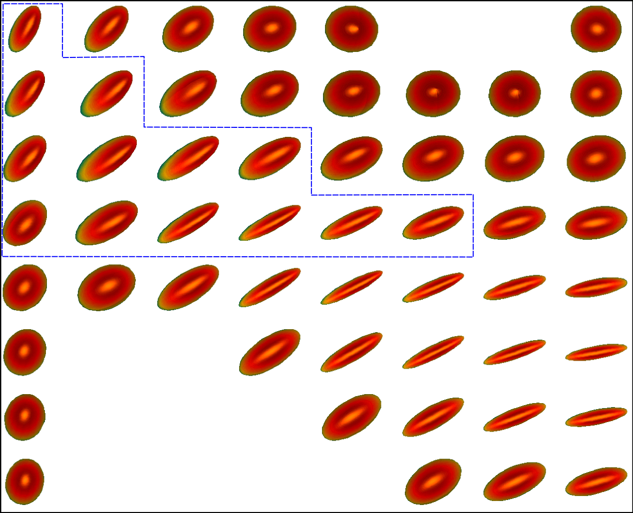 Figure 2
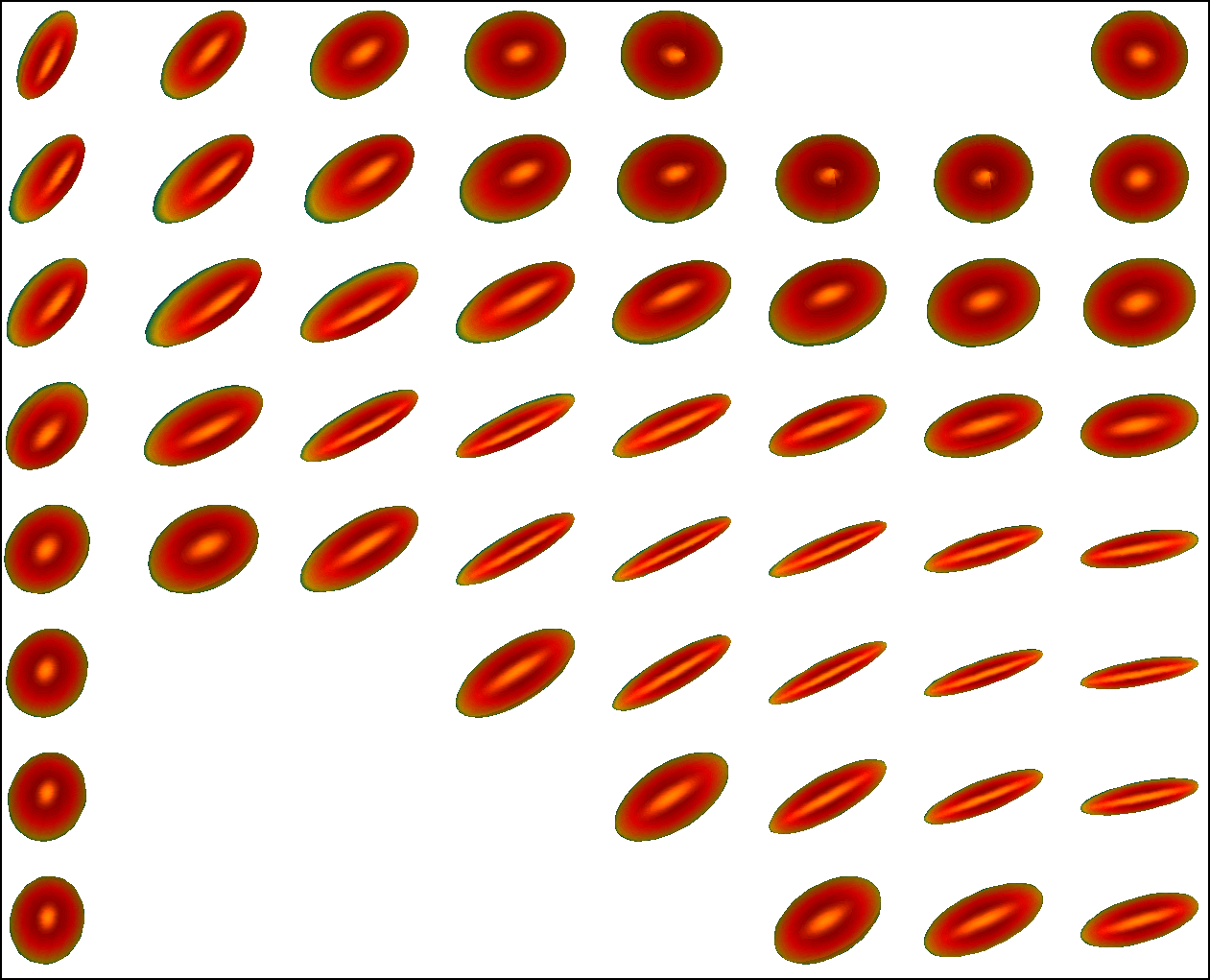 Figure 3
 Figure 4
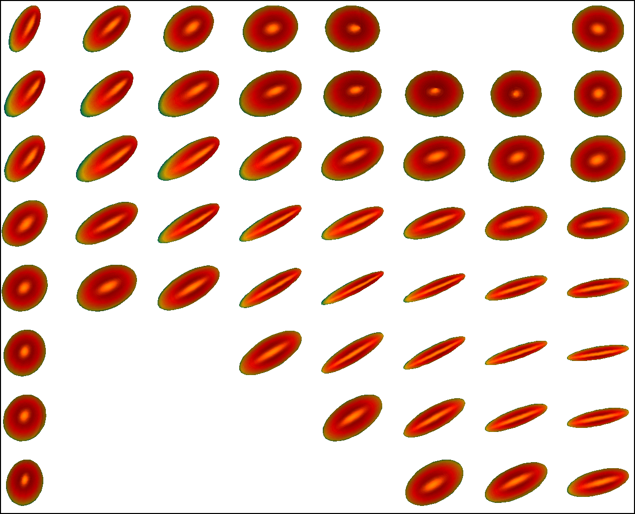 Figure 5
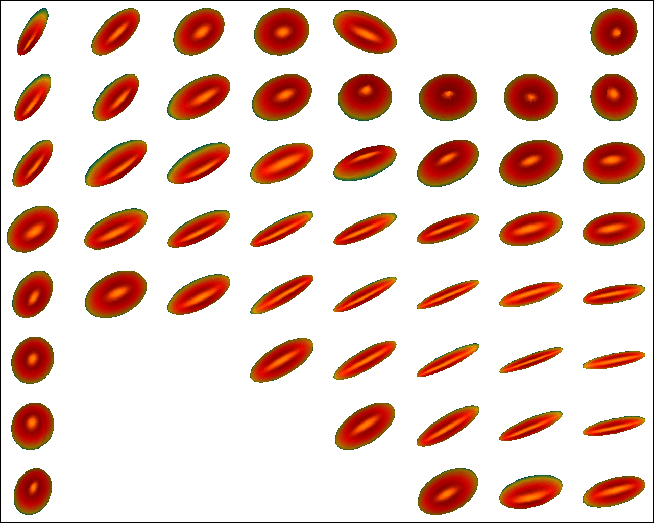 Figure 6
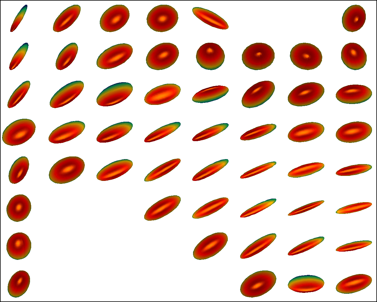 Figure 7
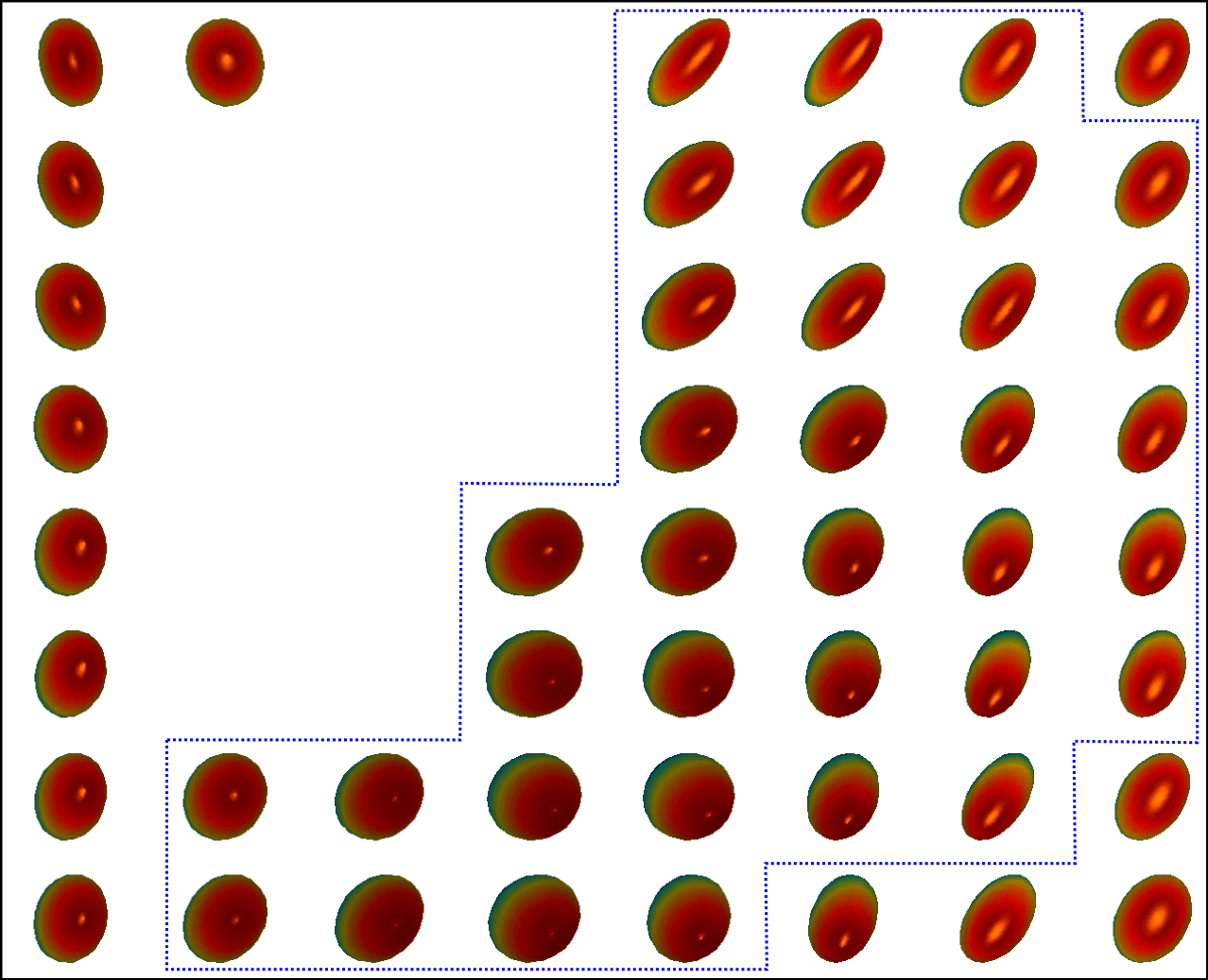 Figure 8
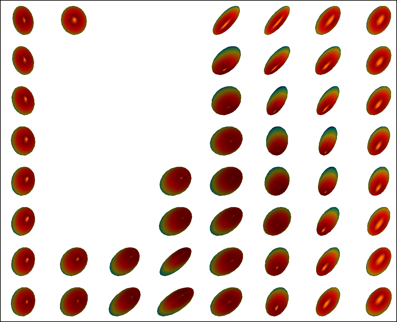 Figure 9
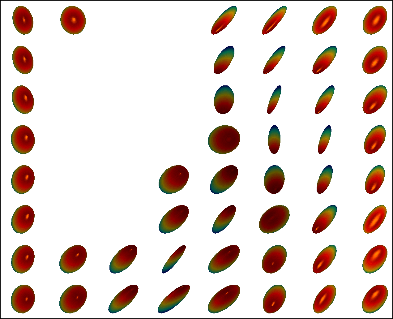 Figure 10
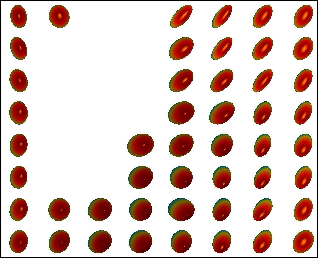 Figure 11
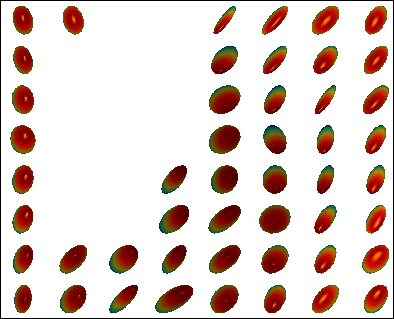 Figure 12
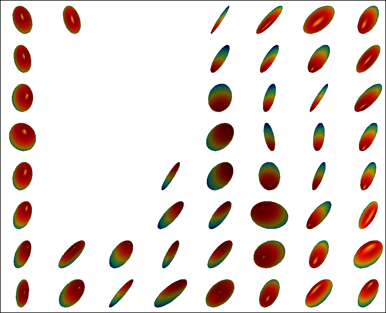 Figure 13
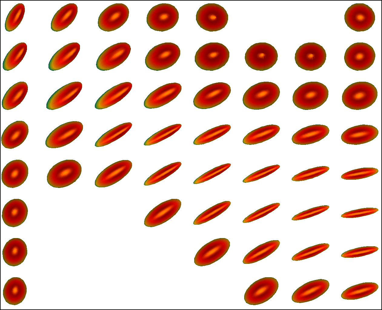 Figure 14
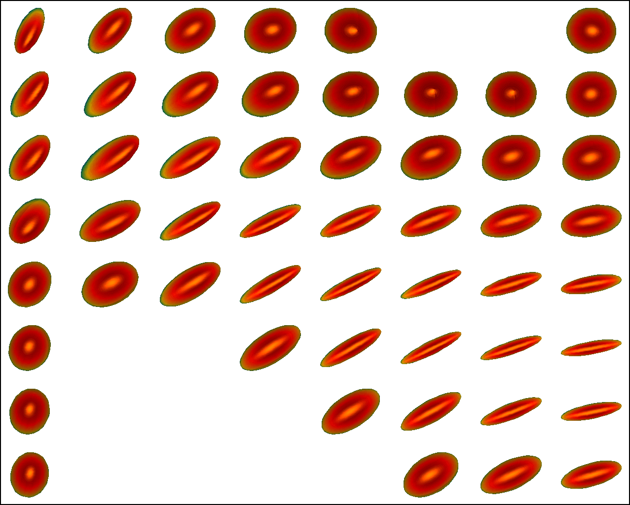 Figure 15
 Figure 16
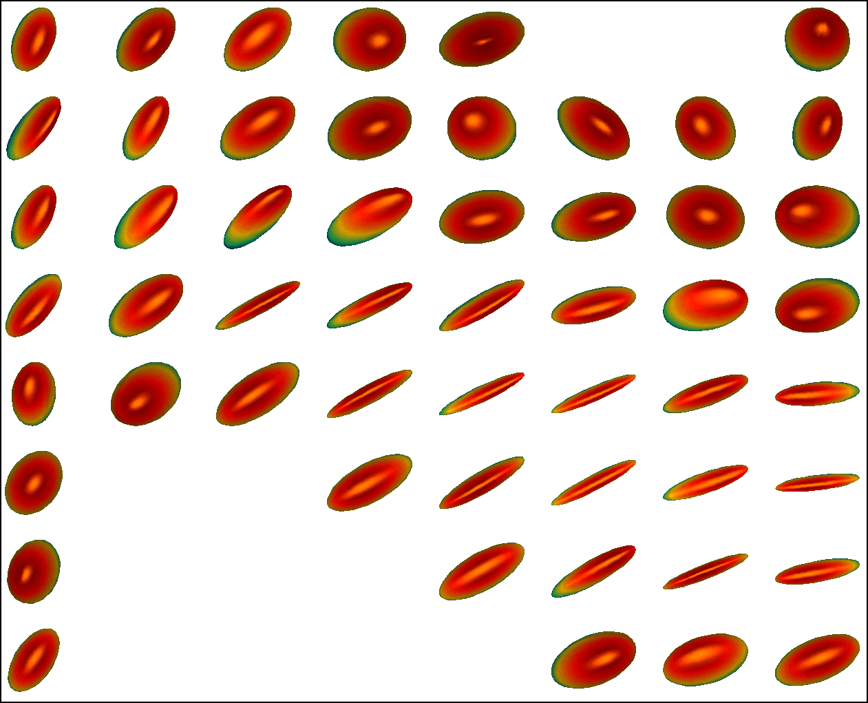 Figure 17
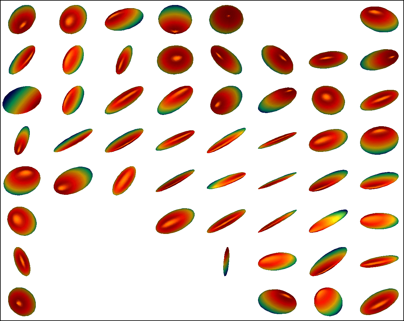 Figure 18
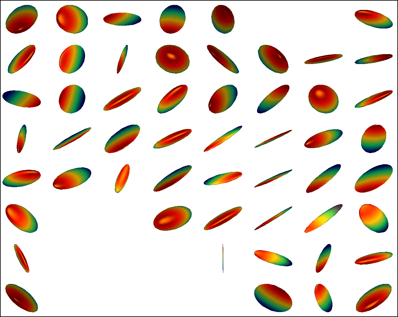 Figure 19
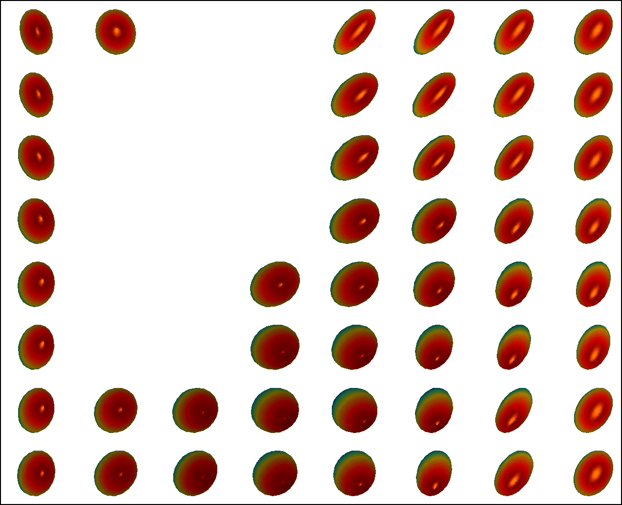 Figure 20
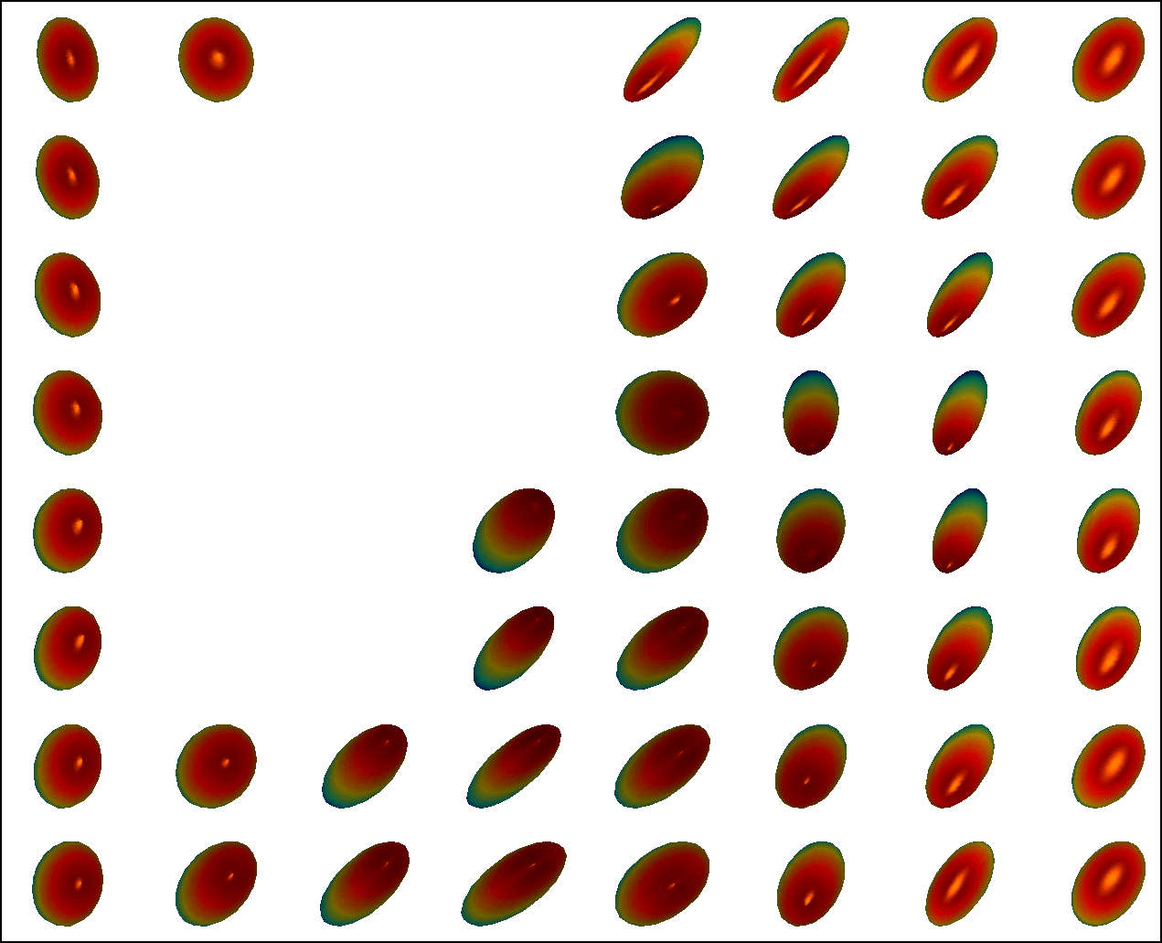 Figure 21
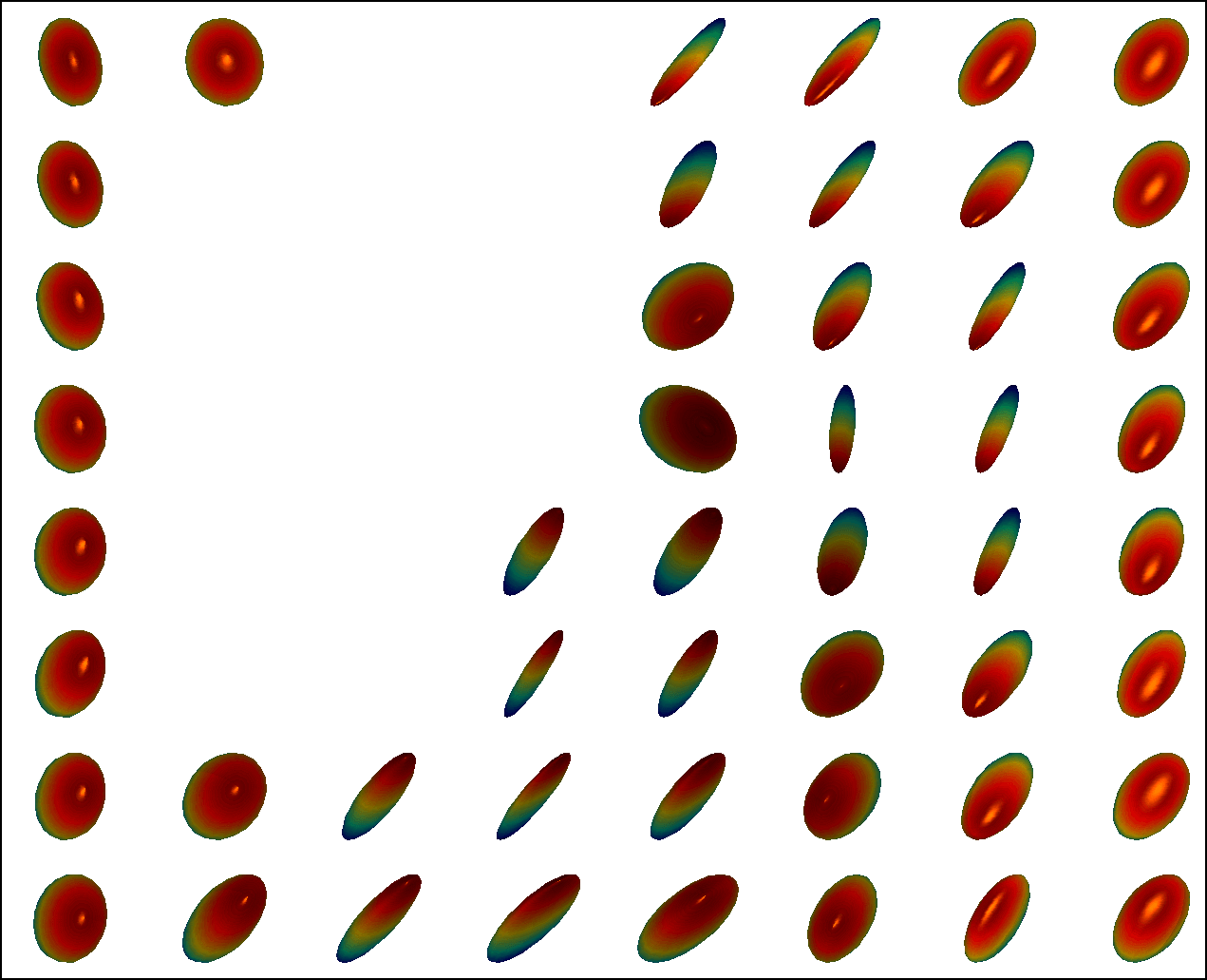 Figure 22
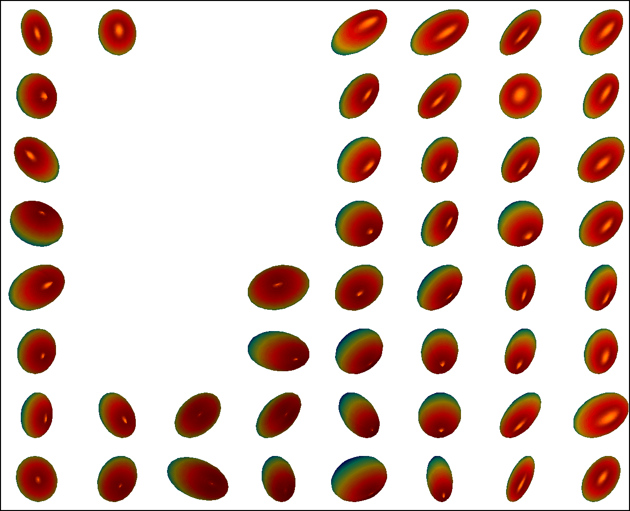 Figure 23
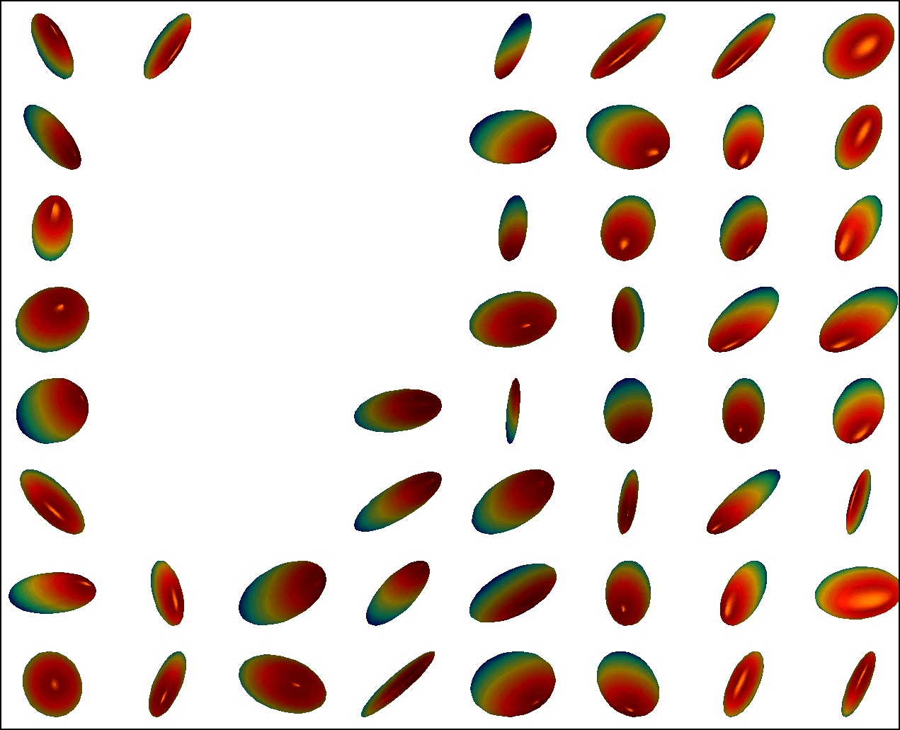 Figure 24
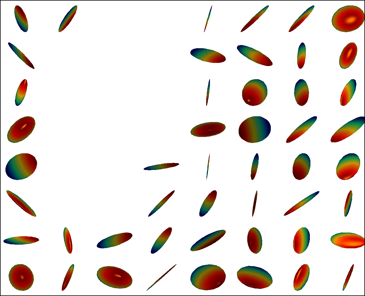 Figure 25
 Figure 26
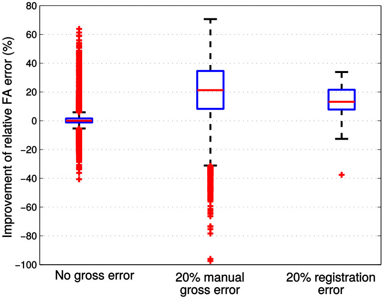 Figure 27
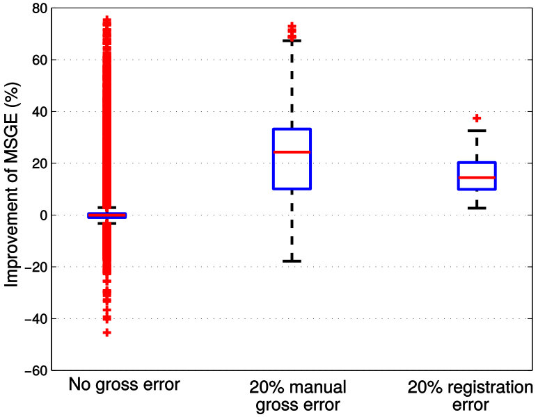 Figure 28
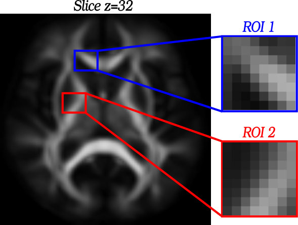 Figure 29
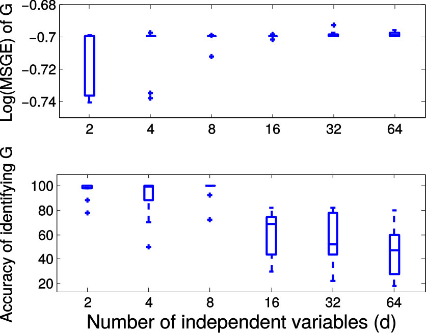 Figure 30
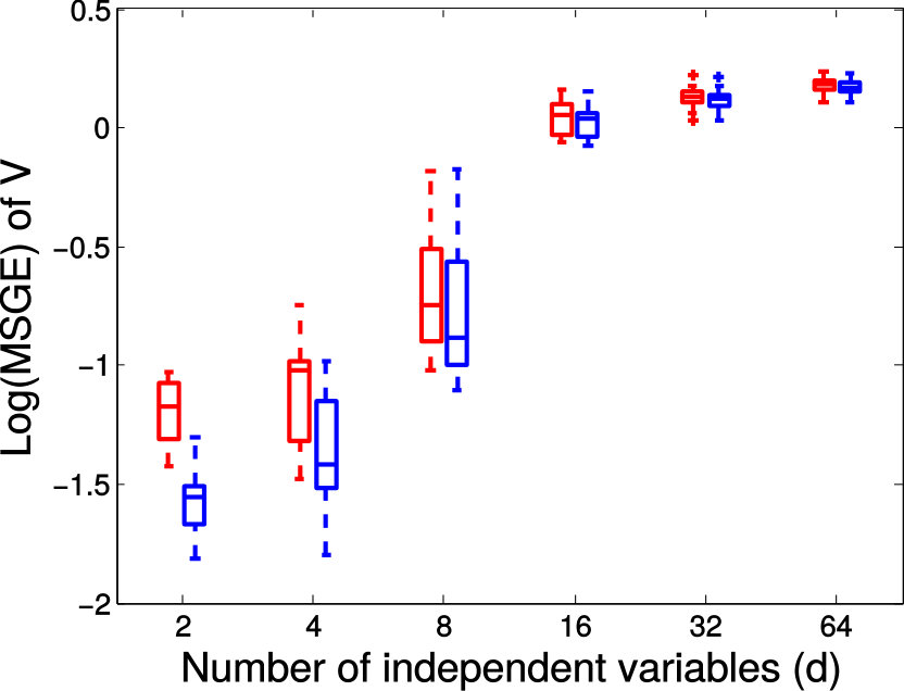 Figure 31
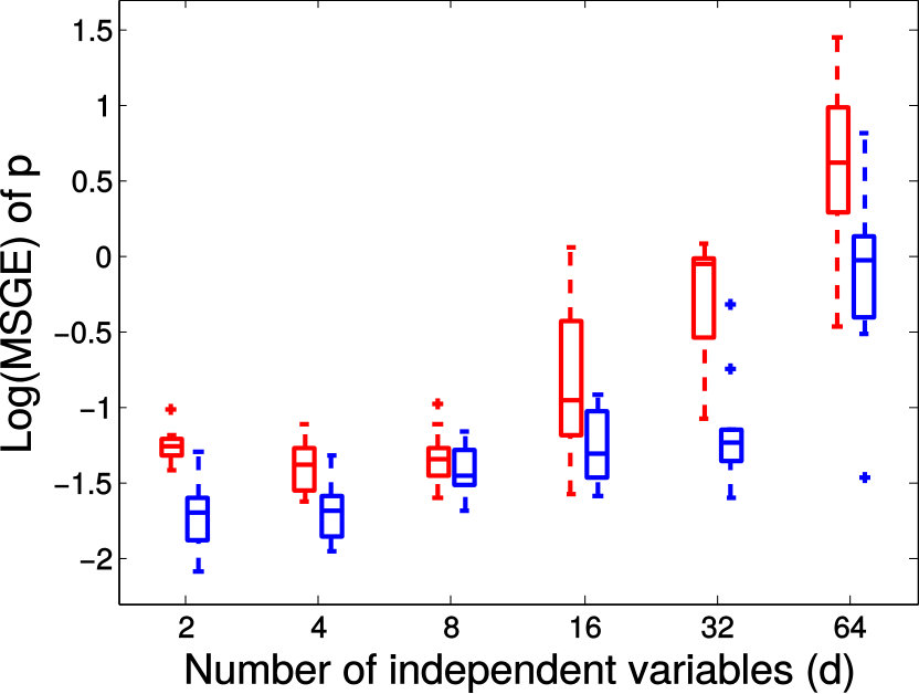 Figure 32
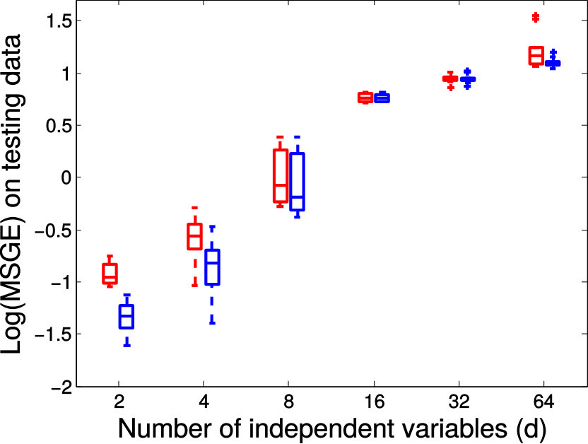 Figure 33
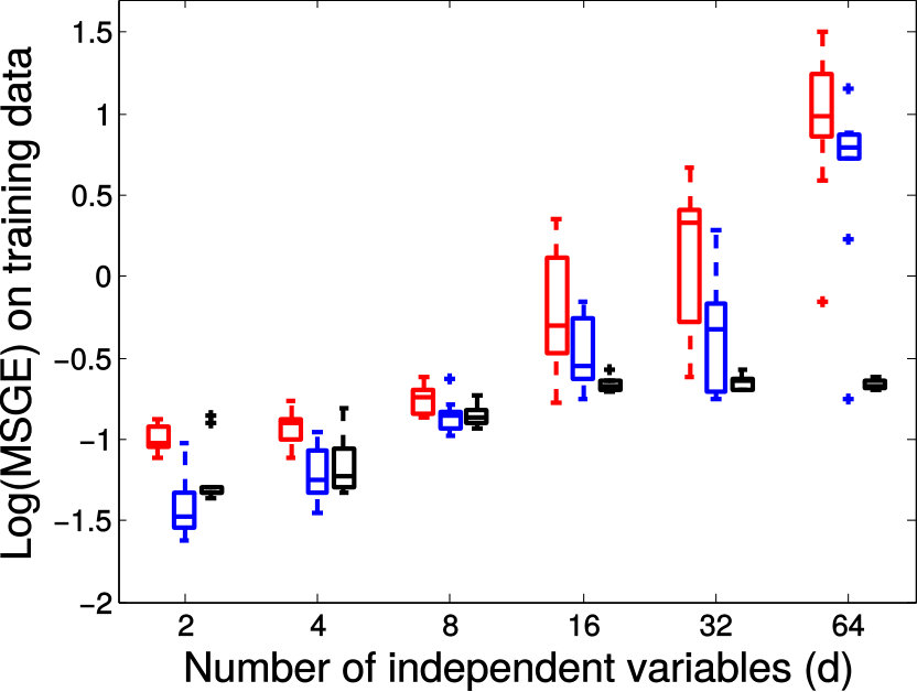 Figure 34
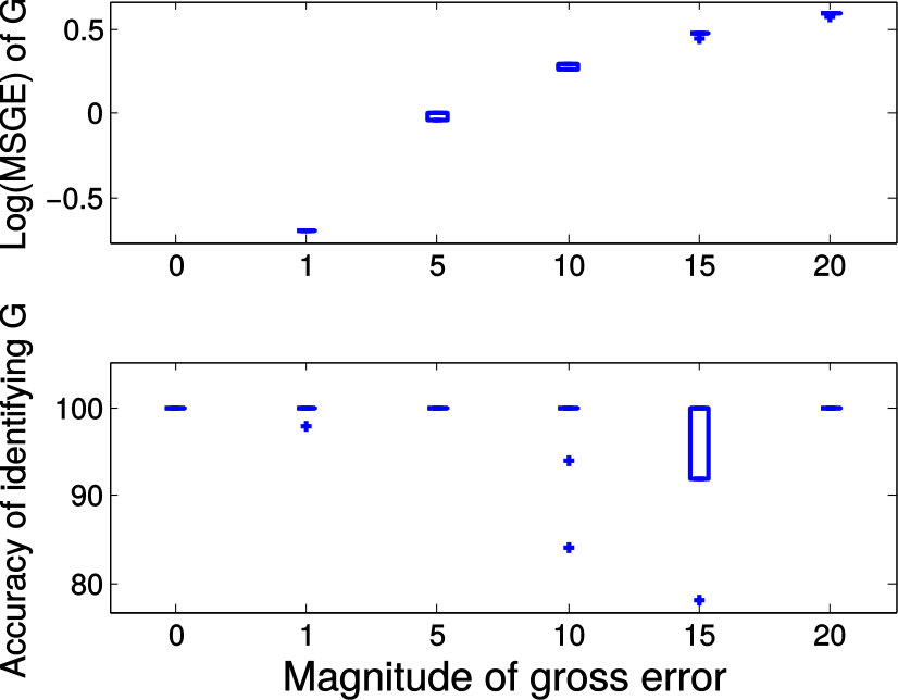 Figure 35
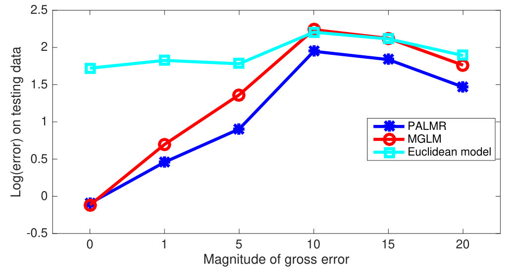 Figure 36
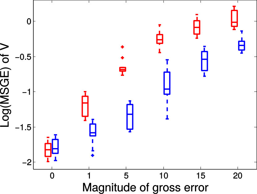 Figure 37
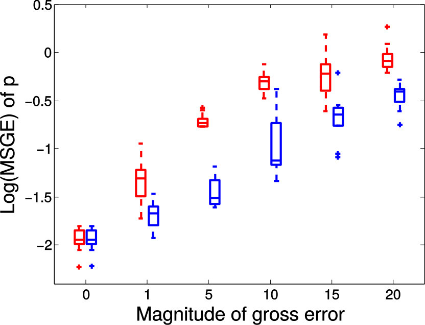 Figure 38
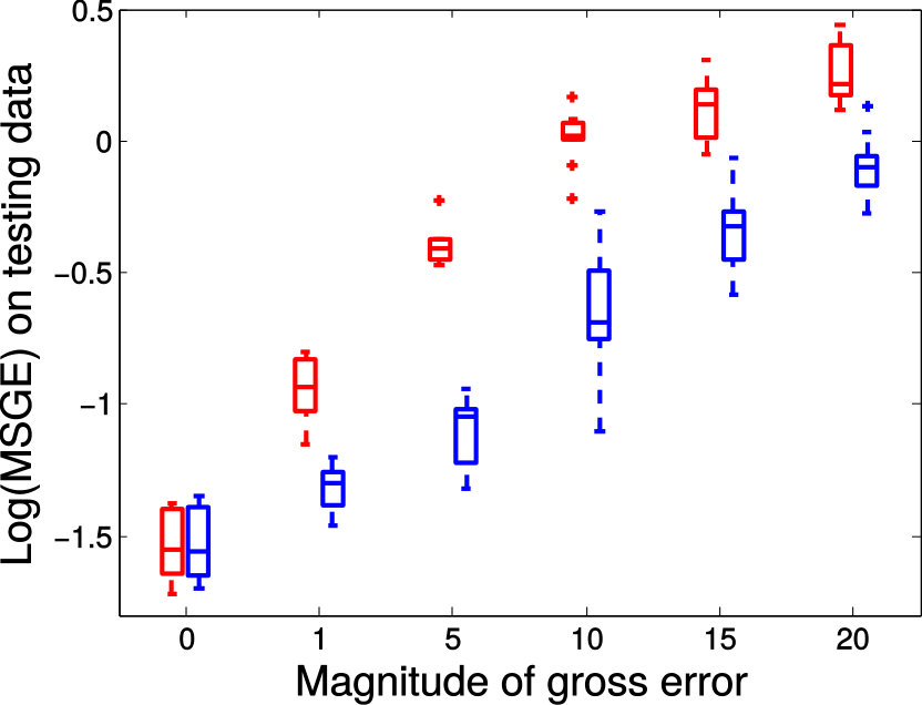 Figure 39
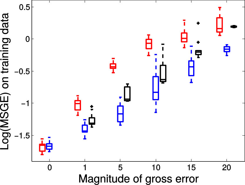 Figure 40
| Metrics | Methods |
|
|
|
||||||||
|---|---|---|---|---|---|---|---|---|---|---|---|---|
| Slice | FA regression | 0.9376 | 1.0414 | 0.9467 | ||||||||
| MGLM | 0.3223 | 0.4349 | 0.1654 | |||||||||
| PALMR | 0.3210 | 0.3409 | 0.1316 | |||||||||
| MSGE | MGLM | 0.1475 | 0.3530 | 0.1949 | ||||||||
| PALMR | 0.1386 | 0.2196 | 0.1508 | |||||||||
| Slice | FA regression | 0.9238 | 1.0362 | 0.8688 | ||||||||
| MGLM | 0.3298 | 0.5089 | 0.2067 | |||||||||
| PALMR | 0.3279 | 0.3682 | 0.1882 | |||||||||
| MSGE | MGLM | 0.1606 | 0.3631 | 0.3513 | ||||||||
| PALMR | 0.1602 | 0.2562 | 0.2915 | |||||||||
| Slice | FA regression | 0.8822 | 1.0136 | 0.9528 | ||||||||
| MGLM | 0.3162 | 0.4564 | 0.1917 | |||||||||
| PALMR | 0.3166 | 0.3665 | 0.1562 | |||||||||
| MSGE | MGLM | 0.1687 | 0.3720 | 0.2449 | ||||||||
| PALMR | 0.1614 | 0.2843 | 0.1906 | |||||||||
| Slice | FA regression | 0.8478 | 1.0066 | 0.8144 | ||||||||
| MGLM | 0.3570 | 0.7342 | 0.2140 | |||||||||
| PALMR | 0.3564 | 0.5081 | 0.1581 | |||||||||
| MSGE | MGLM | 0.1227 | 0.3466 | 0.2954 | ||||||||
| PALMR | 0.1160 | 0.2530 | 0.2445 | |||||||||
| Slice | FA regression | 0.9723 | 1.0526 | 0.9067 | ||||||||
| MGLM | 0.2142 | 0.4053 | 0.5023 | |||||||||
| PALMR | 0.2114 | 0.3318 | 0.4318 | |||||||||
| MSGE | MGLM | 0.1646 | 0.3663 | 0.2436 | ||||||||
| PALMR | 0.1639 | 0.2779 | 0.2226 | |||||||||
| Slice | FA regression | 0.9715 | 1.0695 | 0.9379 | ||||||||
| MGLM | 0.3779 | 0.5976 | 0.1739 | |||||||||
| PALMR | 0.3767 | 0.5319 | 0.1664 | |||||||||
| MSGE | MGLM | 0.2162 | 0.4205 | 0.2928 | ||||||||
| PALMR | 0.2113 | 0.3780 | 0.2593 |
Peer Reviews
No public reviews on file for this paper yet. If you reviewed it on a platform where reviews are public (OpenReview, ICLR, NeurIPS, ICML), you can paste yours below so the community can read it here.
Videos
No videos yet. Explain this paper in a talk, walkthrough, or lecture? Add one.
Taxonomy
TopicsAdvanced Neuroimaging Techniques and Applications · Morphological variations and asymmetry · Bone and Joint Diseases
MethodsLinear Regression
Multivariate Regression with Gross Errors
on Manifold-valued Data
Xiaowei Zhang, , Xudong Shi, Yu Sun, , Li Cheng Xiaowei Zhang is with Bioinformatics Institute, ASTAR, Singapore. E-mail: [email protected] Shi is with School of Computing, National University of Singapore, Singapore. The research is carried out when he is an intern in ASTAR. Yu Sun is with the Singapore Institute for Neurotechnology, National University of Singapore, Singapore 117456. Li Cheng is with Bioinformatics Institute, A*STAR, Singapore (Corresponding author) E-mail: [email protected]
Abstract
We consider the topic of multivariate regression on manifold-valued output, that is, for a multivariate observation, its output response lies on a manifold. Moreover, we propose a new regression model to deal with the presence of grossly corrupted manifold-valued responses, a bottleneck issue commonly encountered in practical scenarios. Our model first takes a correction step on the grossly corrupted responses via geodesic curves on the manifold, then performs multivariate linear regression on the corrected data. This results in a nonconvex and nonsmooth optimization problem on Riemannian manifolds. To this end, we propose a dedicated approach named PALMR, by utilizing and extending the proximal alternating linearized minimization techniques for optimization problems on Euclidean spaces. Theoretically, we investigate its convergence property, where it is shown to converge to a critical point under mild conditions. Empirically, we test our model on both synthetic and real diffusion tensor imaging data, and show that our model outperforms other multivariate regression models when manifold-valued responses contain gross errors, and is effective in identifying gross errors.
Index Terms:
Manifold-valued data, multivariate linear regression, gross error, nonsmooth optimization on manifolds, diffusion tensor imaging.
1 Introduction
This paper focuses on multivariate regression on manifolds [1, 2, 3, 4], where given a multivariate observation , the output response lies on a Riemannian manifold . This line of work has many applications. For example, research evidence in diffusion tensor imaging (DTI) (e.g. [5]) indicates that the shape and orientation of diffusion tensors are profoundly affected by age, gender and handedness (i.e. left- or right-handed). In particular, we consider noisy manifold-valued output scenarios where data are subject to sporadic contamination by gross errors of large or even unbounded magnitude. Such grossly corrupted data are often encountered in practice due to unreliable data collection or data with missing values: For example, errors in DTI data can be introduced by Echo-Planar Imaging (EPI) distortion [6] or inter-subject registration [7], where practical measurement errors such as Rician noise or other sensor noise have a significant impact on the shape and orientation of tensors [8, 9]. Although the problem of learning from data with possible gross error in Euclidean spaces has gained increasing interest [10, 11, 12, 13, 14, 15], to our best knowledge, there exists no prior work in dealing with manifold-valued response with gross errors.
Our main idea can be summarized as follows: For each manifold-valued response , we explicitly model its possible gross error (in ). This gives rise to a corrected manifold-valued data by removing the identified gross error component from , which is realized via geodesic curves on . Note that could be the same as , corresponding to no gross error in . Then the corrected manifold-valued data can be utilized as the responses in multivariate geodesic regression, which boils down to a known problem [2]. More details are illustrated in Figure 1 and are fully described in Section 3. Unfortunately, the induced optimization problem becomes rather challenging as it contains nonconvex and nonsmooth functions on manifolds. Inspired by the recent development of proximal alternating linearized minimization (PALM) methods in Euclidean spaces, in this paper we propose to generalize this technique onto Riemannian manifolds [16], which we have named as PALMR.
The main contributions of this paper are three-fold. First, we propose to address a novel problem of multivariate regression on manifolds where the manifold-valued responses are subject to possible contamination of gross errors. Second, a new algorithm named PALMR is proposed to tackle the induced nonconvex and nonsmooth optimization on manifolds, for which we also provide the convergence analysis. The algorithm and analysis is applicable to a class of nonconvex and nonsmooth optimization problem on manifolds. Empirically our algorithm has been evaluated on both synthetic and real DTI data, where results suggest the algorithm is effective in identifying gross errors and recovering corrupted data, and it produces better predictive results than regression models that do not consider gross errors. Third, our approach makes connections to two established research areas, namely learning from grossly corrupted data and multivariate regression on manifolds: When we restrict ourselves to the special case of Euclidean space, our approach reduces to robust regression considered in e.g. [13, 14]; On the other hand, when there is no gross error, the problem boils down to that of multivariate regression on manifolds as considered in [2], where the method of [2] can be regarded as a special case of our approach. Our code is also made publicly available. 111Our implementation is available at the project website http://web.bii.a-star.edu.sg/~zhangxw/palmr-SPD/.
1.1 Related work
Manifold-valued data arise from a wide range of application domains including neural imaging [17], shape modelling [18, 19, 20], robotics [21], graphics [22], and symmetric positive matrices [23, 24, 25, 26]. One prominent example is DTI [24] where data lie in the Riemannian manifold of symmetric positive definite (SPD) matrices. In this work, we use and to denote the set of symmetric matrices and SPD matrices, respectively. Other examples include higher angular resolution diffusion imaging where data can be modelled as the square root of orientation distribution functions lying on the unit sphere [27, 2], as well as group-valued data such as and in shape analysis [19] and robotics [21]. It is well known that for such scenarios, it is in general much better to conduct statistical analysis directly on the manifold (i.e. curved space) instead of in the ambient Euclidean space (i.e. flat space), which we also verify empirically.
Unsurprisingly, there exists plenty of prior work studying statistics on manifolds [28, 19, 29, 24, 30]. This is to be distinguished from the well-known topic of manifold learning [31], where the data are assumed to be sampled from certain manifold embedded in a usually much higher dimensional Euclidean space and one is supposed to extract intrinsic geometric properties of the manifold from observations. Instead here the manifold is usually known in priori, and the task is to engage appropriate statistical models in the analysis of the manifold-valued data.
In the area of regression on manifolds, Fletcher [28] proposes geodesic regression that generalizes univariate linear regression on flat spaces to manifolds by regressing a manifold-valued response from a real-valued independent data with a geodesic curve. [27] adapts the idea of geodesic regression for regressing sphere-valued data against real scalar. [20] investigates parametric polynomial regression on Riemannian manifolds, while [1] studies regression on the group of diffeomorphisms for detecting longitudinal anatomical shape changes. Banerjee et al. [32] propose a nonlinear kernel-based regression method for manifold-valued data. Hong et al. [33] propose a shooting spline-based regression technique specifically designed for the Grassmannian manifold. [34, 35] investigate a family of nonparametric regression models for data on manifolds. The closest work might be [2], which extends the idea of geodesic regression [28] to multivariate regression on manifolds, and applies it to analyze diffusion weighted imaging data. In [3], the authors investigate multivariate regression models on Riemannian symmetric spaces from a statistical perspective and develop several test statistics for evaluating linear hypotheses of the regression coefficients. In the area of learning with grossly corrupted data, there have been various methods [10, 13, 14, 15, 36] proposed for linear regression with gross errors in the Euclidean space, among which robust lasso in [13] and robust multi-task regression in [14] can be considered as special cases of our approach when restricted to Euclidean spaces.
A recent trend in manifold data analysis is kernel methods on manifolds which aim at embedding the manifold to a reproducing kernel Hilbert space (RKHS). In [37] and [38], kernel methods are developed for sparse coding and dictionary learning on SPD and Grassmann manifolds, respectively. In [39], kernels on SPD and Grassmann manifolds are considered for classification. As it is important for such kernels on manifolds to satisfy the positive definite constraint, significant efforts [40, 41, 42, 43, 44] have been made in this regard. Meanwhile, as shown in [44], these kernels tend to either disregard the original Riemannian structure due to linearization requirement, or violates the positive definiteness constraint. In particular, a geodesic Gaussian kernel is positive definite only if the underlying manifold is Euclidean. Moreover, a geodesic Laplacian kernel is positive definite if and only if conditionally negative definite conditions are satisfied, which is in general not true for curved Riemannian manifolds. These results suggest that the application of kernel methods in curved manifolds has its limitation. On the other hand, it is also of interest for the community to investigate on approaches other than kernel based methods. This motivates us to consider in this work a manifold-valued geodesic regression approach by directly considering the intrinsic Riemannian metric.
2 Background
We first briefly review some concepts in Riemannian manifolds in subsection 2.1, nonsmooth analysis and Kurdyka–Łojasiewicz property on Riemannian manifolds in subsections 2.2 and 2.3, respectively, which are necessary for the derivation of our algorithm and the proof of convergence. We then review some models regarding multivariate linear regression with gross errors in Euclidean space, whose ideas are utilized to design our new model.
2.1 Riemannian manifolds
Let denote a smooth manifold endowed with a Riemannian metric . Moreover, denotes the tangent space at point and denotes the tangent bundle. Notation refers to being a point of and being a tangent vector at . is the inner product between two vectors and in , with being the metric at . The induced norm thus becomes . Let be a piecewise smooth curve such that and , with the curve length as where denotes derivative. The Riemannian distance between and is defined as the infimum of the length over all piecewise smooth curves joining these two points. Let be the Levi-Civita connection 222Roughly speaking, a connection acts as a generalization of directional derivative that connects tangent spaces of nearby points and provides a consistent manner of transporting tangent vectors from one point to another along geodesic curves. A manifold may have many connections. Levi-Civita connection, also called Riemannian connection, is a unique connection that is symmetric and compatible with the Riemannian metric. associated with . Curve is called a geodesic if . A Riemannian manifold is complete if its geodesics are defined for any value of . The parallel transport along from to is a mapping defined by , where is the unique vector field satisfying and . The exponential map at point is a mapping defined as , where is the geodesic such that and . The inverse of the exponential map, if exists, is denoted by . To simplify notations, we also use , , , and to denote inner product, norm, Riemannian distance, and exponential map respectively, when there is no confusion. We focus on Hadamard manifold , which is a complete and simply connected finite dimensional Riemannian manifold with nonpositive sectional curvature. The class of Hadamard manifolds possesses many nice properties: For example, any two points in can be joined by a unique geodesic. In this case, the exponential map is a global diffeomorphism and . One example of Hadamard manifold is the manifold of symmetric positive definite matrices. Motivated readers can consult [45] for further details of manifolds and differential geometry.
2.2 Nonsmooth analysis on Riemannian manifolds
Given an extended real-valued function we define its domain by and its epigraph by . We say that is a lower semicontinuous function if is closed, and is proper if and for all . Proper and lower semicontinuous (PLS) functions play important roles in optimization, since it guarantees the well-definedness of the proximal operator. In particular, given and , the proximal map defined as
[TABLE]
is well-defined when is PLS and . In Section 3, we will see that the objective function in our approach is a PLS. Moreover, we have the following definition of (sub)differential of PLS functions on manifolds.
Definition 1** ([46]).**
Let be a PLS function, then
- •
the Frchet subdifferential of at any , denoted as , is defined as the set of all which satisfies
[TABLE]
for geodesic joining and . When , we set .
- •
the (limiting) subdifferential of at any , denoted as , is defined as
[TABLE]
where is the geodesic joining and .
- •
* is a critical point of if . We denote the set of critical points of by . That is,*
[TABLE]
If is a local minimizer of then by the Fermat’s rule . If is differentiable, then its subdifferential reduces to a unique gradient, denoted as , which is a vector field satisfying for all and . Here denotes the directional derivative of in the direction . In this case . Moreover, we have the following definition of Lipschitz gradients for smooth functions on manifolds:
Definition 2** ([47]).**
Let be a continuously differentiable function and . is said to have -Lipschitz gradient if, for any and any geodesic segment joining and , then
[TABLE]
where , is the parallel transport along from to , and denotes the length of the segment between and . In addition, if is a Hadamard manifold, then the last inequality becomes
[TABLE]
Since is continuously differentiable, and are the unique tangent vectors at and , respectively. Parallel transport thus becomes necessary to move them onto the same tangent space. Note in general, the right hand sides of the two inequalities above are different. This is due to the fact that for non-Hadamard manifolds, geodesic between two points is usually not unique. Since is defined as the infimum length of geodesic segments between and , it could be smaller than , which is the length of the segment between and along a given geodesic . For Hadamard manifolds on the other hand, there exists a unique geodesic between any two points, hence always holds.
2.3 Kurdyka–Łojasiewicz (K-L) property on Riemannian manifolds
The Kurdyka–Łojasiewicz (K-L) property plays a crucial role in nonsmooth analysis [48, 49]. In this subsection we extend the K-L property from Euclidean spaces to Riemannian manifolds. To do this, we need to introduce some basic notations. If is a subset of , then the distance between and is defined by
[TABLE]
where is nonempty, and for all when is empty. For a fixed , the open ball neighborhood of with radius is defined as .
Definition 3**.**
Given real scalars , , and PLS function , we define
[TABLE]
We define similarly .
Now, we define the K-L property.
Definition 4** ([49]).**
Let be a PLS function. The function is said to have K-L property at if there exists , a neighborhood of and a continuous concave function such that
- (i)
, is continuously differentiable on and for all ;
- (ii)
the following K-L inequality holds
[TABLE]
.
We call a K-L function if it has K-L property at each point of .
The K-L property basically asserts that function can be made sharp by a reparameterization of its values using . In particular, when is differentiable and is critical, i.e., , we can define reparameterization , then the K-L inequality becomes , which avoids flatness around . This geometrical feature plays a critical role in proving that the sequence generated by our algorithm converges to a critical point. In Proposition 4 of the supplementary, we also establish K-L property in the neighborhood of non-critical points. K-L functions are ubiquitous in a wide range of applications, including for example semi-algebraic, subanalytic, semiconvex, uniformly convex, and log-exp functions [48, 49].
2.4 Multivariate linear regression with gross errors
Given a matrix representation of observations , and the corresponding -dimensional response matrix , one of the central problems in linear regression is to accurately estimate the regression matrix from
[TABLE]
with being the stochastic noise. In most of existing work regarding linear regression, is assumed to be composed of entries following normal distribution with zero mean. However, when the response is subject to possible gross error, the estimated regression matrix deviates significantly from the true value and becomes unreliable. To deal with this problem, several recent works [12, 13, 14] suggest to consider model
[TABLE]
where is used to explicitly characterize the gross error component. As in practice only a subset of responses are corrupted by gross error, is a sparse matrix whose nonzero entries are unknown and magnitudes can be arbitrarily large. Moreover, this model can as well be applied to deal with the case where some entries of are missing. A commonly used paradigm of estimating is by solving convex optimization problem
[TABLE]
where and are tuning parameters, and and are regularization terms of and , respectively. Some frequently used regularization norms include norm which is the summation of the absolute value of all entries, and norm which is the summation of norm of rows of a matrix. For example, in [14] the authors propose to use and .
3 Our Approach
Consider a set of training examples , where lies on Riemannian manifold and is the associated independent variable. We propose a novel extension of the modeling approach of Eq. (2) for Euclidean spaces to deal with the more general curved spaces, as follows.
3.1 From Euclidean spaces to manifolds
The Model of Eq. (2) can be reformulated as . Denote , which can be interpreted as corrected response after removing the gross error. Now the model of Eq. (2) can be reformulated as standard linear regression in Eq. (1) with response . With this in mind, we proceed to extend the aforementioned idea to regression on manifolds. For each manifold-valued response , denote as its corrected version. Different from the Euclidean space setting where can be obtained from simply by a translation, we need to ensure that remains on the manifold. This is accomplished by the exponential map with the gross error over each of the training examples, . Note that when is an Euclidean space, the exponential map reduces to addition, as . In other words, translation in the affine space is a special case of exponential map in the more general curved space.
As illustrated in Figure 1, we first obtain the corrected manifold-valued response . Then the relationship between and can be modeled as
[TABLE]
where and is a set of tangent vectors at , is the component of , and is a tangent vector at . Our model can be viewed as a generalization of linear regression model of Eq. (1) from flat spaces to manifolds, where denotes the intercept that is in analogy to the origin [math] in the flat space as in Eq. (1), and exponential map corresponds to the addition operator in Eq. (1).
To measure the training loss, we use
[TABLE]
to denote the sum-of-squared Riemannian distance between the corrected data and the prediction , and let and denote two regularization terms controlling the magnitude of and , respectively. The problem considered in our paper can now be formulated as the following optimization problem
[TABLE]
where and are regularization parameters. Without loss of generality, we consider regularization terms and , with and being the norm of tangent vectors at and , respectively. There are two reasons for the choice of : First, it enables problem of Eq. (7) to contain the multivariate linear regression problems with feature selection in Euclidean spaces as special cases, as shown in Example 1 and Example 2 below; Second, in many applications one may collect a large set of possible variables for each response, and want to find a compact subset of base tangent vectors from and the corresponding that are significant to the manifold-valued output . The choice of is based on the assumption that gross errors are usually sporadically spread among data. Now, the optimization problem becomes
[TABLE]
3.2 Connections to existing works
We would like to point out that model in Eq. (11) includes as special cases a number of related research works on gross error or on manifold-valued regression. In this subsection, we provide three such examples.
Example 1**.**
When , we can establish a connection between the model of Eq. (11) and the robust multi-task regression studied in [14]. Specifically, instead of optimizing Eq. (11) over we select , resulting in
[TABLE]
which can be rewritten as
[TABLE]
where becomes the usual Euclidean norm, , , and . The resulting model of Eq. (12) is exactly the one considered in [14] except that regularization term in [14] is replaced by here.
Example 2**.**
If , we can show by Fermat’s rule that the optimal solution is given by . By substituting into problem of Eq. (11) and assuming has empirical mean [math], that is, and , the optimization problem of Eq. (11) reduces to
[TABLE]
which can be reformulated as
[TABLE]
where is a column vector with all entries being 1.
The difference between Example 1 and Example 2 lies in that the former is obtained from selecting while the latter is from optimizing which exactly follows model of Eq. (11). The resulting models are quite similar except that model of Eq. (2) needs to center variable .
Example 3**.**
If we let and , then optimization problem of Eq. (11) reduces to
[TABLE]
which recovers exactly the model considered in [2]. In this regard, the MGLM model in [2] is a special case of our model.
3.3 PALM for optimization on Hadamard manifolds
In this subsection, we propose a new algorithm to solve optimization problem of Eq. (11), which is actually a nonsmooth optimization problem on Hadamard manifolds. As explained in details in subsection 3.4, problem of Eq. (11) admits the form
[TABLE]
where and are Hadamard manifolds, and are PLS functions, and is a smooth function.
Many existing optimization techniques are developed to work with Euclidean spaces, thus not directly applicable to curved manifolds. Meanwhile, an increasing amount of attention has been drawn to the field of optimization on manifolds [50]. For smooth optimization, classical optimization techniques, such as gradient, conjugate gradients, and trust-region methods, have been generalized to the manifold setting [50, 51, 52, 53], which are however not suitable for the nonconvex and nonsmooth optimization manifold-based problem of Eq. (11). For nonsmooth optimization, there exist many prior works [54, 55, 56, 57]. Unfortunately they either cannot exploit the composition structure in Eq. (14) (e.g., [54, 55, 57]), or fail to guarantee convergence (e.g., [56]).
Recently, a proximal alternating linearized minimization (PALM) algorithm has been proposed in [16] for optimization problem of Eq. (14) with and . Inspired by the success of PALM in the Euclidean setting, in what follows we propose PALMR, an inexact proximal alternating minimization algorithm for problem of Eq. (14).
We alternately solve the following two proximally linearized subproblems
[TABLE]
where and with , and , being the Lipschitz constants of and , respectively, as to be explained in Assumption 1. In particular, by exploiting the fact that is a Hadamard manifold on which any two points can be joined by a unique geodesic, we have a one-to-one mapping between and such that , and . Thus, a simple substitution reformulates Eq. (15) as
[TABLE]
or equivalently,
[TABLE]
which becomes an optimization problem in linear space , and as a result, we have . Since is PLS satisfying and is smooth, it follows that the composite function is PLS and which, together with Theorem 1.25 of [58], implies that is well-defined. Moreover, the above optimization problem for is called proximity operator [59], denoted as
[TABLE]
Similar claims apply to problem of Eq. (16), implying the well-definiteness of and . Solving Eqs. (15) and (16) alternately yields the algorithm PALMR outlined in Algorithm 1.
To analyze the convergence of PALMR, we need the following assumptions.
Assumption 1**.**
* satisfies the following conditions:*
- (i)
, and .
- (ii)
For any fixed , the function has -Lipschitz gradient. Likewise, for any fixed , the function has -Lipschitz gradient. Moreover, there exist real scalars for , such that
[TABLE]
- (iii)
* is Lipschitz continuous on bounded subset of . More specifically, for bounded subset , there exists constant such that for all , , we have*
[TABLE]
- (iv)
* has the Kurdyka–Łojasiewicz (K-L) property on Hadamard manifolds.*
Assumption (i) establishes that proximal operators in Eqs. (15) and (16) are well-defined, leading to the well-definedness of algorithm PALMR. Assumption (ii) provides that is locally block-Lipschitz continuous, and the boundedness of Lipschitz constants are to ensure sufficient decrease of objective function value over iterations. Assumption (iii) considers the partial gradients of being Lipschitz continuous, which would be used to derive lower bound for the iteration gap + . Assumption (iv) guarantees that form a Cauchy sequence.
Under Assumption 1 we have the following theorem, whose proof is provided in the supplementary.
Theorem 1**.**
Suppose Assumption 1 holds. Let be a sequence generated by PALMR. Then either the sequence is unbounded or the following assertions hold:
The sequence has finite length, i.e. and .
- 2)
The sequence converges to a critical point of .
Based on Theorem 1, we know that the sequence generated by PALMR converges to a critical point of , provided the boundedness of the sequence. As shown in [16], there are many scenarios where such assumption holds. For example, when functions and are convex and where and are matrices, then the sequence is bounded.
In what follows, we specifically investigate the dedicated realization of PALMR to solve the optimization problem of Eq. (11). To simplify the notation, the resulting algorithm is also referred to as PALMR when there is no confusion.
3.4 Applying PALMR to optimization problem of Eq. (11)
Optimization problem of Eq. (11) in our context can be reformulated as
[TABLE]
which is of the form in Eq. (14) with and . To apply PALMR to solve problem of Eq. (11), we need to evaluate the gradients of . To simplify the notation, we further denote the prediction \hat{\bm{y}}_{i}:=\mathrm{Exp}_{\bm{p}}\big{(}\sum_{j}x_{i}^{j}\bm{v}_{j}\big{)}, as well as the derivatives of the exponential map with respect to and as and , respectively. Now, the partial gradient of with respect to amounts to
[TABLE]
where is the adjoint derivative of the exponential map [28] defined by \big{\langle}\bm{\mu},d_{\bm{p}}\mathrm{Exp}_{\bm{p}}(\bm{v})\bm{w}\big{\rangle}_{\mathrm{Exp}_{\bm{p}}(\bm{v})}=\big{\langle}\big{(}d_{\bm{p}}\mathrm{Exp}_{\bm{p}}(\bm{v})\big{)}^{{\dagger}}\bm{\mu},\bm{w}\big{\rangle}_{\bm{p}} with , . The adjoint derivative operator maps from the tangent space of to the tangent space of . Thus . Similarly, the partial gradient of with respect to and are given by
[TABLE]
and
[TABLE]
respectively.
The PALMR algorithm for problem of Eq. (11) proceeds as follows: To update , we let and and solve
[TABLE]
where is the parallel transport from to along the unique geodesic between them. Due to the constraint , it is difficult to solve and together. Instead, the above subproblem is solved by alternating minimization over and . Specifically, to update , we solve
[TABLE]
which, by a change of variable , is equivalent to solving
[TABLE]
and .
To update , we need to first obtain by
[TABLE]
where . Notice that the above optimization problem have closed form solution of
[TABLE]
where if and [math] otherwise. Since lie on the tangent space at , we need to parallel transport them to by along the unique geodesic between and .
Similarly, update by
[TABLE]
where .
Now, we are ready to present our algorithm for multivariate regression with grossly corrupted manifold-valued data, as shown in Algorithm 2. Notice that when letting and , Algorithm 2 alternately updates the values of and via three steps: (1) , (2) , (3) , which recovers the gradient descent method proposed in [2].
3.5 Implementation of Algorithm 2
During each iteration of Algorithm 2, the partial derivatives , and of Eqs. (17), (18), and (19) are evaluated. Their detailed derivations are provided in Section 3 of the supplementary file. Nevertheless, these terms could be practically intractable to compute for some manifolds, due to the presence of adjoint derivatives of the exponential map. As a remedy to this issue, we adopt the variational technique of [2, 60] for computing derivatives, which basically replaces the adjoint derivative operators by parallel transports:
[TABLE]
One advantage of such approximation is that for some special manifolds, including manifold of SPD matrices , parallel transports have analytical expressions and can be computed directly. For general manifolds that have no analytical expressions for parallel transports, approximation approaches such as Schild’s ladder approximation [61, 62] can be used. The method approximates parallel transport by constructing geodesic parallelograms, which requires three exponential maps and two inverse exponential maps, as shown in Figure 2.
4 Experiments
In this section, we empirically evaluate the performance of the proposed approach (i.e. PALMR) in working with synthetic and real DTI data sets, which lies in the manifold of SPD matrices. Throughout all experiments, we fix and choose the optimal from set by a validation process using a validation data set consisting of the same number of data points as the testing data. As our algorithm is iterative by nature, in practice it stops if either of the two stopping criteria is met: (1) the difference between consecutive objective function values is below 1e-5, or (2) maximum number of iterations (100) is reached.
4.1 Synthetic DTI data
Synthetic DTI data sets are constructed with known ground-truths and gross errors as follows: First, we randomly generate , symmetric matrices and where entries of are sampled from standard normal distribution . Then the ground-truth DTI data is obtained as . This is followed by DTI data with stochastic noise as , where is a random matrix in with its entries being sampled from and satisfies . Meanwhile, the gross errors are generated by a two-step process: (a) Randomly select an index subset from , such that with . (b) For , its grossly corrupted response is attained by , where is a random matrix in satisfying . The rest of the training data remain unchanged, i.e. for . Thus, among all manifold-valued data, the percentage of grossly corrupted data is . With the same and , we also generate pairs of testing data and validation data.
We first conduct experiments on a data set with , , and , and compared with the multivariate general linear model (MGLM) of [2] which has not considered gross error. Training samples are displayed in Figure 3, where we also show the predictions of PALMR and MGLM on the training data. Visual results of PALMR and MGLM on 20 testing data and training data correction by PALMR are presented in Figure 4(a) and Figure 4(b), respectively. Collectively, the results suggest that PALMR indeed is capable of correctly identifying the gross errors during training. This enables the delivery of a better-behaved model. Figure 4(b) shows that PALMR can effectively recover the original data (i.e. true data without gross error). It also produces improved regression results on testing data as displayed in Figure 4(a).
Next we quantitatively evaluate the effect of varying the internal parameters of PALMR, which include the number of independent variables , the number of training data , magnitude of gross error , and percentage of grossly corrupted training data . To see the effect of one specific parameter, synthetic DTI data are generated by varying this parameter value while keeping rest parameters at their default values. The following default values are used: , , , and . To evaluate performance of PALMR, the following mean squared geodesic error (MSGE) metrics are considered: , , , , and , where , and are the outputs of Algorithm 2. The data correction error is measured as . In addition, we say that gross error is correctly identified if both and are either zero or nonzero, and compute the rate . Results averaged over 10 repetitions are presented in Figure 5, where each column corresponds to the effect of one parameter and each row corresponds to the results using one metric.
From Figure 5, we have four observations: (1) PALMR has lower MSGE for all values of , and our correction performs well on training data, cf. column Figure 5(a). (2) PALMR has large advantage over MGLM for all values of training size () and magnitude of gross error (), cf. columns Figure 5(b-c). (3) PALMR can handle training data with up to being grossly corrupted, and delivers better result than MGLM. On the other hand, the performance is slightly worse if more than of training data are corrupted, cf. column Figure 5(d). (4) PALMR can reliably identify most of the gross errors. Still it may not always correctly recover the true value of the error. This is evidenced in the last row of Figure 5, where the MSGE on increases as or increases, and our correction error starts to stand out (i.e. being larger than both prediction errors of PALMR and MGLM) when over of the training samples are grossly corrupted. We believe this is acceptable as in most practical situations, only small fraction of the training examples would be contaminated by gross errors.
Finally, we compare the proposed method PALMR and MGLM with an Euclidean multivariate linear regression model with gross errors described in equation (12) of Example 1. All experimental settings are the same as above except three aspects: (i) Since the Euclidean model can not deal with DTI tensors directly, for each tensor , we vectorize its upper triangle part into a 6-dimensional vector. Therefore, and in model (12). (ii) Since predictions of the Euclidean model are not guaranteed to lie on the SPD manifold, the geodesic metrics are not applicable. As alternate, we adopt Frobenious norm distance to measure the distance between prediction and ground-truth . (iii) We only investigate the effect of the magnitude of gross errors and the ratio of gross errors in the training data. Results are shown in Figure 6, where the -axis in each plot denotes the log-scale of median error over 10 reptitions measured by Frobenious norm. We observe that PALMR achieves the best performance and outporforms the Euclidean model by a large margin under various settings. MGLM also performs better than the Euclidean model, but when there are large gross errors in the training data, its advantage disappears, as can be seen in the left plot. These observations are within our expectation, since the Euclidean model does not respect the intrinsic structure of the DTI data.
4.2 Real DTI data
In this section, we apply PALMR to examine the effect of age and gender on human brain white matter. We experiment with the C-MIND database 333https://cmind.research.cchmc.org released by Cincinnati Children’s Hospital Medical Center (CCHMC) with the purpose of investigating brain development in children from infants and toddlers (0 3 years) through adolescence (18 years). We use the imaging data of participants who were scanned at CCHMC at year one and whose age were between 8 and 18 (2947 to 6885 days), consisting of 27 female and 31 male. The DTI data of each subject are first manually inspected and corrected for subject movements and eddy current distortions using FSL’s eddy tool [63], then passed to FSL’s brain extraction tool to delete non-brain tissue 444http://fsl.fmrib.ox.ac.uk/fsl/fslwiki/. After the pre-processing, we use FSL’s DTIFIT tool to reconstruct DTI tensors. Finally, all DTIs are registered to a population specific template constructed using DTI-TK 555http://dti-tk.sourceforge.net/pmwiki/pmwiki.php. We investigate six exemplar slices that have been identified as typical slices by domain experts and have been also similarly used by many existing works such as [2, 27]. And in particular, we are interested in the white matter region. At each voxel within the white matter region, the following multivariate regression model
[TABLE]
is adopted to describe the relation between the DTI data and variables ‘age’ and ‘gender’.
In DTI studies, another frequently used measure of a tensor is fractional anisotropy (FA) [64, 65] defined as
[TABLE]
where , and are eigenvalues of the tensor. FA is an important measurement of diffusion asymmetry within a voxel and reflects fiber density, axonal diameter, and myelination in white matter. In our experiments, we also compared three models: two geodesic regression models, MGLM and PALMR, and the FA regression model which uses FA value to replace tensor in Eq. (23). The relative FA error metric is employed to compare the results of geodesic regressions and FA regression, as follows: Since the responses of geodesic regression are tensors, the FA values of the tensors can be computed. The relative FA error metric is then evaluated on testing data, which is defined as the mean relative error between the FA values of the predicted tensors and the true tensors. Besides this relative FA error metric, the aforementioned mean squared geodesic error (MSGE) on testing data as in subsection 4.1 is still engaged to compare the performance of MGLM and PALMR.
4.2.1 Model significance
To examine the significance of the statistical model of Eq. (23) considered in our approach, the following hypothesis test is performed. The null hypothesis is , which means, under this hypothesis, age has no effect on the DTI data. We randomly permute the values of age 666Empirical results investigating the effect of ‘gender’ are provided in Section 5 of the supplementary file. among all samples and fix the DTI data, then apply model of Eq. (23) to the permuted data and compute the mean squared geodesic error , where is the prediction of PALMR on the permuted data. Repeat the permutation times, we get a sequence of errors and calculate a -value at each voxel using . Figure 7 presents the maps of voxel-wise -values for three models using six typical slices, and Figure 8 displays the distribution of -values for all six slices collectively.
As shown in Figure 7 and Figure 8, geodesic regression models are able to capture more white matter regions with aging effects than FA regression model. In addition, voxels satisfying -value are more spatially contiguous when geodesic regression models are used, as can be seen from the zoom-in plot for each slice in Figure 7. This may be attributed to the fact that geodesic regression models preserve more geometric information of tensor images than that of FA regression. We also observe that PALMR and MGLM obtain very similar results. This is to be expected, as both methods use model of Eq. (23) and adopt geodesic regression on manifolds. The main difference is that PALMR considers gross error while MGLM does not, and in this experiment, there is no gross error in the DTI data.
4.2.2 Model predictability
We proceed to investigate the predictability of PALMR when compared with existing methods such as FA regression and MGLM. For each of the six slices, we randomly partition our data into 40 training (20 female + 20 male) and 18 testing (7 female + 11 male) data, then train all three methods on each voxel within the white matter region. To test the ability of PALMR in handling gross errors, we consider three different experimental settings: (1) No gross error, where all training data are fully preprocessed as described at the beginning of subsection 4.2; (2) 20% manual gross error, where for each voxel we randomly select of training instances and insert gross error with magnitude ; (3) 20% registration error, where of the patients in the training data are randomly selected to undergo an incomplete registration processing. Compared with fully preprocessed data, DTI data with registration error are obtained by skipping the diffeomorphic registration step in DTI-TK. The purpose of experimenting on data with registration error is to imitate the realistic scenario that gross error can be caused by improper preprocessing of the data. We should remark that registration error is more challenging to handle than the manual gross error, since its magnitude varies dramatically for different voxels and patients. A heat map of registration error for each slice is provided in Fig. 1 of the supplementary file. In this case, instead of considering all voxels on each slice, we set a threshold value and consider those voxels whose minimum registration error is greater than . For the first four slices, we set and for the last two slices we set . The three comparison methods are examined on the three types of training data, and for each voxel the experiments are repeated 10 times.
TABLE I provides the median values of prediction errors measured with both relative FA error and MSGE on all voxels and over all six slices. As clearly indicated in TABLE I, geodesic regression models again outperform FA regression model, which is to be expected. Moreover, when there is no gross error in the training data, both MGLM and PALMR achieve similar results. This is consistent with the claim that MGLM is a special case of PALMR when there is no gross error. In addition, the ‘20% manual gross error’ column shows that when of the training data contain gross errors PALMR outperforms MGLM by a large margin. For the challenging case of 20% registration error, the last column of TABLE I shows that PALMR is still much better than its competitors. In Figure 9, we use box plots to demonstrate the performance advantage of PALMR over its competitors. For each metric, the performance improvement is computed as (error of the best competitor - error of PALMR) / error of the best competitor * 100%. Figure 9 displays the same results as in TABLE I from a different perspective and with more details. We first compute the performance improvement of PALMR on each voxel of all six slices to get a percentage value, then put all values under the same metric and experimental setting to plot a box plot. Figure 9 shows that PALMR improves the median prediction error by at least 20% and 15% in the case of manual gross error and registration error, respectively.
The distribution of prediction errors measured by the relative FA error and the MSGE on each slice is shown in Figure 10 and Figure 11, respectively. In each plot, the method with corresponding distribution on the left is better than the one with corresponding distribution on the right. From both Figure 10 and Figure 11, we get similar observation as in TABLE I. Moreover, Figure 11 shows that PALMR is more robust to gross errors than its competitors. In Fig. 2 of the supplementary file, we also show the comparison of prediction errors of MGLM and PALMR on each voxel of all slices. We observe that on most of the voxels PALMR is better than MGLM when gross errors are present. More experimental results on real DTI data are available in Section 5 of the supplementary file.
5 Conclusion and Future Work
This paper focuses on the interesting problem of multivariate regression on manifolds with gross error contamination, where mathematical formulation nevertheless resides in a challenging landscape concerning a nonconvex and nonsmooth optimization on manifolds. A new algorithm, PALMR, is proposed to address this problem and its convergence property is analyzed. Through empirical studies, PALMR is shown to be capable of dealing with the presence of gross error and produces reliable results. For future work, there are several directions to explore. In terms of theoretical study, it remains to investigate the recoverbility of the proposed model, that is, to study conditions under which our model can correctly locate gross errors and recover their magnitude. It is also of interest to analyze the asymptotic behaviour of the resulting estimators. In terms of applications, in addition to age and gender, one may also consider the influence of handedness (i.e. left- or right-handed) on DTI responses. We also plan to apply our framework to different applications including shape analysis and robotics, where the manifolds of interest could be and .
The reference list from the paper itself. Each links out to its DOI / PubMed record.
- 1[1] B. C. Davis, T. Fletcher, E. Bullitt, and S. C. Joshi, “Population shape regression from random design data,” International Journal of Computer Vision , vol. 90, no. 2, pp. 255–66, 2010.
- 2[2] H. Kim, N. Adluru, M. Collins, M. Chung, B. Bendlin, S. Johnson, R. Davidson, and V. Singh, “Multivariate general linear models (MGLM) on Riemannian manifolds with applications to statistical analysis of diffusion weighted images,” in CVPR , 2014.
- 3[3] E. Cornea, H. Zhu, P. Kim, J. Ibrahim, and the Alzheimer’s Disease Neuroimaging Initiative, “Regression models on Riemannian symmetric spaces,” Journal of the Royal Statistical Society: Series B (Statistical Methodology) , vol. 79, no. 2, pp. 463–482, 2017.
- 4[4] P. Muralidharan and P. T. Fletcher, “Sasaki metrics for analysis of longitudinal data on manifolds,” in CVPR , 2012.
- 5[5] J. Hsu, A. Leemans, C. Bai, C. Lee, Y. Tsai, H. Chiu, and W. Chen, “Gender differences and age-related white matter changes of the human brain: A diffusion tensor imaging study,” Neuro Image , vol. 39, no. 2, pp. 566–577, 2008.
- 6[6] M. Wu, L.-C. Chang, L. Walker, H. Lemaitre, A. Barnett, S. Marenco, and C. Pierpaoli, “Comparison of EPI distortion correction methods in diffusion tensor MRI using a novel framework,” in MICCAI , 2008.
- 7[7] A. Zalesky, “Moderating registration misalignment in voxelwise comparisons of DTI data: a performance evaluation of skeleton projection,” Magnetic Resonance Imaging , vol. 29, no. 1, pp. 111–125, 2011.
- 8[8] M. Bastin, P. Armitage, and I. Marshall, “A theoretical study of the effect of experimental noise on the measurement of anisotropy in diffusion imaging,” Magnetic Resonance Imaging , vol. 16, no. 7, pp. 773–785, 1998.