A Solitonic Approach to Holographic Nuclear Physics
Salvatore Baldino, Stefano Bolognesi, Sven Bjarke Gudnason, and Deniz, Koksal

TL;DR
This paper uses holographic models to analyze nuclear physics, revealing classical soliton descriptions of baryons, their interactions, and bound states, including the deuteron, within a large N_c and large lambda framework.
Contribution
It introduces a solitonic approach to holographic nuclear physics, computing nuclear bound states and their properties in the Sakai-Sugimoto model at large N_c and lambda.
Findings
Classical solitons describe baryons in the model.
Bound states for baryon numbers up to eight are characterized.
The deuteron state is identified as a quantized zero mode.
Abstract
We discuss nuclear physics in the Sakai-Sugimoto model in the limit of large number of colors and large 't Hooft coupling . In this limit the individual baryons are described by classical solitons whose size is much smaller than the typical distance at which they settle in a nuclear bound state. We can thus use the linear approximation outside the instanton cores to compute the interaction potential. We find the classical geometry of nuclear bound states for baryon number up to eight. One of the interesting features that we find is that holographic nuclear physics provides a natural description for lightly bound states when is large. For the case of two nuclei, we also find the topology and metric of the manifold of zero modes and, quantizing it, we find that the ground state can be identified with the deuteron state. We discuss the relations with other methods…
Click any figure to enlarge with its caption.
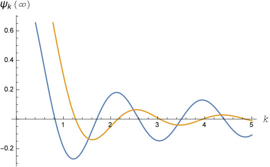 Figure 1
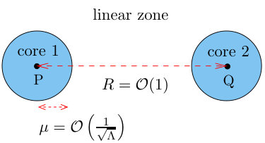 Figure 2
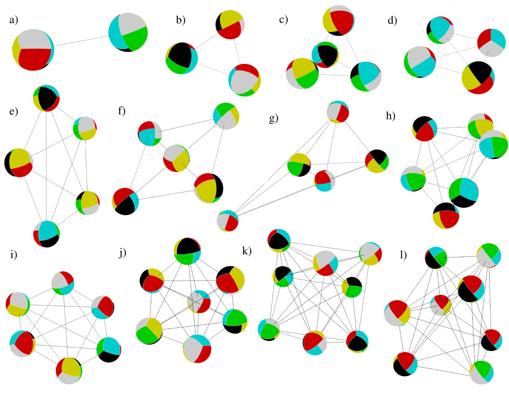 Figure 2
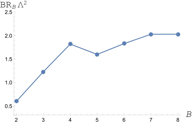 Figure 4
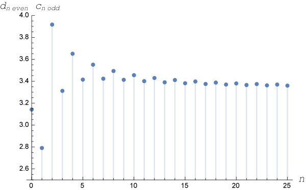 Figure 5
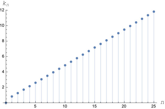 Figure 6
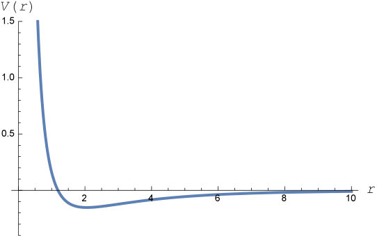 Figure 7
| Shape | Details | |||
| Line | Distance = | |||
| Equilateral triangle | Side = | |||
| Tetrahedron | Side = | |||
| Square | Side = | |||
| Pentagon | Side(outer) = | |||
| (Tetrahedron + | Tetrahedron (Base = , Sides = ), | |||
| Satellite) | Satellite (increasing) = () | |||
| Cross | Distance from the center = | |||
| Square + 2 satellites | Tetrahedron = ((base: ),), | |||
| Distance from the two satellites = | ||||
| ((to base: ), | ||||
| (to roof: )) | ||||
| Hexagon | Side (outer) = | |||
| Tetrahedron | Pyramid Base = (,,,), | |||
| + triangle | Distance to the satellites = | |||
| () | ||||
| () | ||||
| () | ||||
| Two twisted squares | Square sides = (2.34,3.85) | |||
| Twisted node connections(increasing) = | ||||
| (2.63,3.19,3.72,4.51) | ||||
| Two rectangles | Rectangles: | |||
| Base = (2.03,4.45), Roof =(2.38,4.04) | ||||
| Distance between closest nodes = | ||||
| (3.49,3.57,3.49,3.57) |
Peer Reviews
No public reviews on file for this paper yet. If you reviewed it on a platform where reviews are public (OpenReview, ICLR, NeurIPS, ICML), you can paste yours below so the community can read it here.
Videos
No videos yet. Explain this paper in a talk, walkthrough, or lecture? Add one.
IFUP-TH-2017
A Solitonic Approach to Holographic Nuclear Physics
Salvatore Baldino*(1), Stefano Bolognesi(1), Sven Bjarke Gudnason(2)*
and Deniz Koksal*(1)*
*(1)**Department of Physics “E. Fermi”, University of Pisa and INFN Sezione di Pisa
*Largo Pontecorvo, 3, Ed. C, 56127 Pisa, Italy
*(2)**Institute of Modern Physics, Chinese Academy of Sciences, Lanzhou 730000, China
emails: [email protected], [email protected],
[email protected], [email protected]
(March 2017)
Abstract
We discuss nuclear physics in the Sakai-Sugimoto model in the limit of large number of colors and large ’t Hooft coupling . In this limit the individual baryons are described by classical solitons whose size is much smaller than the typical distance at which they settle in a nuclear bound state. We can thus use the linear approximation outside the instanton cores to compute the interaction potential. We find the classical geometry of nuclear bound states for baryon number up to eight. One of the interesting features that we find is that holographic nuclear physics provides a natural description for lightly bound states when is large. For the case of two nuclei, we also find the topology and metric of the manifold of zero modes and, quantizing it, we find that the ground state can be identified with the deuteron state. We discuss the relations with other methods in the literature used to study Skyrmions and holographic nuclear physics. We discuss and corrections and the challenges to overcome to reach the phenomenological values to fit with real QCD.
Contents
1 Introduction
The Sakai-Sugimoto (SS) model is a holographic dual model of QCD [1, 2]. It is a top down approach and consequently has very few parameters to fit. Flavor dynamics are encoded in the low energy action for the gauge field on the flavor branes, and the baryons of QCD are the instantonic configurations of that gauge theory [3, 4, 6, 5]. Quantization of the degrees of freedom for an instantonic field of charge one creates a quantum system of states, whose transformation properties and quantum numbers are just right to interpret them as nucleons. Nuclear physics at low energy is thus turned into a multi-instanton problem in a curved five-dimensional background; this is the problem we discuss in the present paper. We will approach the problem of nuclei in the SS model from a “solitonic perspective”, in a way somehow different, or complementary to other approaches which already exist in the literature [7, 8, 9, 10, 11, 12, 13, 14]. We shall use many techniques developed in the context of nuclei within the Skyrme model, for example [15, 16, 18, 19, 20, 21, 22, 23, 24].
The limit which we consider is that of the large number of colors and large ’t Hooft coupling . The instanton radius scales as and, as we shall verify a posteriori, the distances between individual nuclei in the bound state configuration scale as . This suggests us to use a linear approach for the computation of the dominant two-body potential between the nuclei. Our first result is that nuclear physics at large and large does have bound states in the linear regime. In this picture, we build a charge two field configuration by “gluing” together two single charge instanton solutions, where by gluing we mean taking the linear superposition. In the large and limit we compute exactly the energy of this field configuration and interpret the result as the potential of interaction between nuclei. This is proposed as a classical potential for the baryon interaction, where its structure as an infinite sum of Yukawa monopole and dipole interactions is interpreted as the classical analogue of the exchange interaction with a meson mediator. We show how classical nuclei with multiple baryons can be described in this limit. The solution has some analogies with the one obtained recently in a lightly bound Skyrme model [25, 26]. We confront our potential with the one obtained in [8] through a different approach and explain the differences and the limits of validity for the various approaches at hand.
Focusing then on the two-nuclei system, we quantize the coordinates of the two instanton fields and impose physical constraints in order to restrict the spectrum of the system. We see that the internal degrees of freedom of the system can be rearranged and interpreted as the total spin and the isospin of the system, and that they assume only integer values. Among the states that are compatible with our constraints, we find one with the right angular quantum numbers (spin one and isospin zero) to be interpreted as the deuteron.
In section 2, we review the low energy action of the SS model, concentrating on the solitonic solutions of the theory. In section 3, by gluing together two solutions at large spatial separation, we find a classical interaction potential between the nucleons. We then generalize to topological sectors of arbitrarily high charge. In section 4 the system is quantized and we show that the minimal energy state in the spectrum has the same quantum numbers as the deuteron. In section 5 we discuss various types of corrections from the inclusion of the massive modes. We conclude in section 6.
2 Holographic baryons in the Sakai-Sugimoto model
We take, as a starting point, the low-energy action of the SS model, which is a five dimensional gauge theory in a particularly curved background. We call the gauge field , and its associated field strength tensor . In these terms, we are studying a field theory of the form
[TABLE]
where the space-time has the topology of , and the metric is given by
[TABLE]
and the warp factor, , is
[TABLE]
From now on, we adopt the units of . The action is given by
[TABLE]
The term in the second integral is the Chern-Simons term. is the number of colors from the dual QCD and it is an overall multiplicative constant of the above action. The classical equations of motion are thus completely independent of and the quantum corrections are negligible when we take the limit.
We divide the field into two components: an abelian and a non-abelian part . Similarly for the field strength
[TABLE]
We rescale the action as
[TABLE]
and define the new coupling
[TABLE]
Furthermore, we restrict to the case of two flavors for simplicity. The rescaled action reads
[TABLE]
2.1 Classical baryon solution
We want to find static solutions of this theory. To do so, we perform the static ansatz as
[TABLE]
that is, we remove all dependence of time coordinates from the fields and the field . In this ansatz, we also suppose that is not a propagating field, but a constrained field fixed by the equations of motion. With this ansatz, the action reads
[TABLE]
and the equations of motion are
[TABLE]
where is the covariant derivative with respect to the field . The last equation defines as the inhomogeneous solution of the equation, obtained through convoluting the Green function of the LHS operator with the RHS.
To have a finite action solution, the non-abelian gauge field must approach a pure gauge configuration on the sphere at infinity, :
[TABLE]
As , we have a discrete (but infinite) number of topological sectors, labeled by the topological charge
[TABLE]
that assumes integer values. We have an additional constrained field, , that can be interpreted as an electrostatic potential for the electric field , sourced by the topological charge.
We review the solution for the sector [4, 5]. We assume a central ansatz , with , even if the curvature along the direction explicitly breaks invariance with respect to translations along . We make the ’t Hooft ansatz
[TABLE]
where
[TABLE]
The appropriate boundary conditions to have finite energy and are
[TABLE]
Inserting the ansatz in the action and developing in orders of we see that, at order in the scaled action and neglecting warp factors, we have the same action of the BPST instanton:
[TABLE]
where represents the instanton size, which is a modulus for the standard BPS instanton. The rescaled energy is given by
[TABLE]
The energy of the instanton then grows with its size, and with the gravitational effect alone the instanton becomes pointlike and placed at . The instanton would shrink to zero size, would it not be for the Chern-Simons term: the abelian field acts as an effective electric potential, and as the topological charge density is positive everywhere the net effect of the electric field is to expand the instanton. Those two effects combine to give an instanton of definite classical size
[TABLE]
As the energy is size dependent, is not a modulus for the SS instanton, and it is fixed to the value (2.21) unless stated otherwise. is given by
[TABLE]
In normal units, the soliton has energy (that we interpret as rest mass)
[TABLE]
The presence of a gauge field used to stabilize a soliton is not a peculiarity of this model, and it has been amply studied as an alternative term used to stabilize the Skyrmion, see for example [16, 17].
We now turn our attention to the moduli space of zero modes. We have explicit translational invariance along the coordinates, so we have three moduli , indicating the position of the instanton in physical space. We also have global gauge transformations, which do not fall off to zero at infinity. We get as the moduli space
[TABLE]
The calculation of the metric on the moduli space is similar to the standard calculation for the standard BPS instanton, and the result is the same [4]. It reads
[TABLE]
where is the standard metric. The instanton size and the coordinate along the direction are massive moduli.
2.2 The linear regime
We now perform an expansion in . The objective is to find an expression for the fields and the equations of motion (2.11), (2.12) and (2.13) and identify the linear region of the soliton, the region of space where we can approximate the gauge potential with its first term in the expansion [6, 5].
We define the approximation through
[TABLE]
where each term is of order . We are interested in the equations of motion for the field . In the linear zone (which is given by ), we can take only the contributions to the action and the equations of motion, effectively linearizing the system.111Actually, the linear approximation is valid up to : in the region the contributions with become more important than , so the linear approximation breaks down in that region [5]. We will consider the situation where and neglect that zone. Before proceeding, we divide the field
[TABLE]
where the superscript indicates parity with respect to : the part is an even function, in the gauge where the core potential has been obtained, so . Restricting to the order terms in the equations of motion (and dropping the superscript), we have
[TABLE]
where the source terms are delta functions or derivatives, centered at . By developing the core solution to first order in , we obtain explicit expressions for and use them to calculate the source terms.
To proceed, we define the functions to solve the equation
[TABLE]
for some numbers . We define the scalar products
[TABLE]
This way, by partial integration, we can see that
[TABLE]
we can just set . The obey the differential equation
[TABLE]
We can numerically calculate the functions in the following way. Let be the asymptotic value for of an even solution to (2.32) with in place of , and let be the same for odd functions. Searching for normalizable solutions of (2.32) then amounts to finding the zeroes of and . We plot those functions in Fig. 1. The zeroes of are the entries of with odd , while the zeroes of are the entries of with even .
There is a subtlety: if we set , we see that is a solution. We also have that converges, and it has the value , so we can include in the expansion of . We note that the primitive of , that would be , still solves , but does not fall off at infinity and is not normalizable under the scalar product .
We impose for odd and for even, where the prime is the derivative with respect to . This way, we have that . We define
[TABLE]
where and have to be determined numerically. As we have . The only particular value is the norm of : we have , while is divergent. In the potential we will have to use as coefficients the with odd and the with even. We plot the values of the pulses and the alternating succession of and in Figure 2.
With the previous choice of normalization, the completeness relations are
[TABLE]
We thus define, following [6], the Green functions
[TABLE]
which obey
[TABLE]
We now take the linear approximation to the core solution from [5]. In terms of the functions and , they can be written as
[TABLE]
We now apply the operators of the linear equations of motion, obtaining the form of the source terms:
[TABLE]
We can generalize the linear form with an arbitrary phase and an arbitrary position, : this is done by substituting with (and analogously for ), and every occurrence of the Pauli matrices with . We will use this linear form of the fields in the following when calculating the interaction potential between nuclei.
3 Nucleon-Nucleon potential and classical nuclei
We now perform the calculation of the holographic potential between nucleons. To do so, we place the instantons with their cores at a distance from each other, which we assume to be greater than and we set both holographic coordinates for the two instantons to zero in order to minimize the energy. The system is diagrammatically shown in Figure 3. We write the single instanton fields by writing the first one as in (2.40) and writing the second one by translating it to and assigning an arbitrary phase matrix to it. We call , the gauge field centered in the origin, , and , the gauge field centered in . Due to the distance between the fields, we can take the gauge field in the whole space to be : in the “core 1” region, is small and can be considered as a small perturbation, while the opposite situation happens in “core 2”. There is a linear zone where both fields are weak, and can be both approximated by their linear form.
3.1 The interaction potential
The energy of the configuration can be found by using the fact that the field can be approximated by the sum of two fields and one of the coefficients of the sum can always be taken as a linear perturbation. We start by writing the scaled energy, through an integration by parts:
[TABLE]
In the integration by parts, we have used the fact that the functions are supposed to vanish at the boundaries fast enough for the energy to be finite. We split this integral into two: we will see that the first two terms (called ) give the dipole interaction contribution, while the last one (called ) gives a monopole interaction.
Let us start with the evaluation of the monopole term
[TABLE]
where is the Laplace-Beltrami operator
[TABLE]
In our approximation, we can divide the topological charge density as , so that we also divide the gauge field into , such as , and similarly for . The monopole term (3.2) becomes
[TABLE]
The terms contribute to the self energies of the instanton and we neglect them as we are really interested in the cross terms in order to obtain the potential. Let us then take . is peaked in the zone, where must be taken as its linear approximation. We can then suppose to be strongly localized at through the delta function: . In this approximation, the topological charge of the soliton is still one. Any contribution that tends to enlarge the soliton comes from the electrostatic field, and is then multiplied by some negative power of : as we are keeping the linear order in we can neglect those contributions. With the functions, the integral is easily performed and we can do the same with the other term too. Summing everything and removing the self energies, we obtain the monopole part of the potential. Using the linear form of the fields, we have
[TABLE]
This is the monopole potential, where only the contribution of with odd matters. This monopole interaction can be interpreted as a classical analogue of the exchange potential between the instantons, which interact by exchanging mesons with masses .
The contribution of the dipole part can be calculated through a trick, similar to the one used in [21]. Dividing the space into (core 1), (core 2) and (linear zone), we split the integral as
[TABLE]
In the region, we can take, as a first approximation, the whole gauge field to be coincident with . Then, we relax this approximation by admitting variations of the form , always taking the first order in . The integral over the region of the unperturbed field is a contribution to its self energy, while the variation of this energy accounts for the interaction between the instantons and consequently is the only piece that we need. The variations that we need are:
[TABLE]
where we denote the field strength and the covariant derivative built from as and respectively. We can do the same in the and region, interchanging the roles of the two fields. Noting
[TABLE]
we can write
[TABLE]
Since the gauge field in the core region goes as for great and so does the linear approximation, we can approximate the covariant derivative with the usual one. We can then use Stokes’s theorem, using the fact that , to get
[TABLE]
where is a vector field normal to , pointing outwards (remember that is a ball in four dimensions). In the region , both fields take their linear form, so we can linearize the field strength tensors (neglecting the commutator) and approximate every with their linear approximations. We use Stokes’ again to return inside the region. Derivatives act only on the field strength, as when they act on the gauge field, the first term cancels the second one. Using the linear equations of motion, we have , as we are integrating in the region and the core of is outside of it. Performing the division in parity components, we get the integral
[TABLE]
Using the equations of motion (2.2), we see that the operators in the parentheses, when applied to the fields, give terms proportional to a Dirac delta function, such that the integrals are simply done by evaluating at the origin and then adding the necessary constants and derivatives.
The first line of the potential reads
[TABLE]
Here we have used the explicit form of (2.21) in order to obtain the dependence, just as we did with the monopole term. The matrix is equal to
[TABLE]
This term can be interpreted as the sum of Yukawa dipole interactions between the two instantons, mediated by the infinite tower of mesons, , which have the same masses as the mesons. While the monopole interaction is always repulsive, the dipole interaction depends on the phase matrix , which is interpreted as the isorotation that we must perform on the first object in order to obtain the same iso-orientation from the second object.
The last part of the potential comes from the last two lines of (3.1). They are combined in the term
[TABLE]
There are some fundamental differences between and . The first one is the overall sign. The second is the fact that we are also including a contribution: as , contains a massless, long range interaction. The particle that we classically take as the mediator of this long range interaction is the pion, which is massless in our model. The other mesons, of mass , are interpreted as a tower of mesons.
Now that we have a final result for the interaction potential, we scale back to physical units and perform some changes in order to have a more generalized result which we will use in the following sections. We denote the coordinates of the first instanton by , and the coordinates of the second instanton by , where are 3-vectors and and are matrices. The field configuration described by this coordinate configuration is
[TABLE]
We make the change of variables: and , as is usually done in two-body problems: hence the potential will only depend on the relative distance . It is also easy to find out that has to be substituted simply by , indicating the relative orientation of the two objects. We define the symmetric tensor
[TABLE]
with on the RHS indicating the modulus of the position vector, and express the potential as
[TABLE]
We have separated the pion contribution from the rest of the meson tower and used explicitly and .
3.2 Looking for a bound state: the classical deuteron
We can obtain a classical description of the deuteron by looking for a minimum energy configuration, where we choose the coordinates of our instantons to minimize (3.17).
We have to choose the relative orientation of the instantons. To do that, it is useful to switch to the axis-angle notation in order to write the rotation matrix . As is an matrix, it can be specified by giving two components of a versor, the axis of rotation (where the third component is decided from the normalization of the vector, with a positive sign), and an angle , indicating the rotation around the versor (counterclockwise). We can then express any as
[TABLE]
The orientation dependent part is then given by
[TABLE]
We need a negative contribution from the dipole part to contrast the monopole part. Our best bet is to choose , along with and , such that we get a positive contribution from , as that would mean that the long range force mediated by the pion is attracting the two objects, in contrast to the potential. We then choose the configuration of phase opposition, where and are orthogonal and indicates a half rotation: we can choose , and , which corresponds to . This leads to . We will choose and as the phase opposition configuration (numerical analysis confirms that the global minimum is attained in phase opposition). The potential in this channel is plotted against the distance between the two instantons in Figure 4. We also calculate the asymptotic behaviors of the potential in the and limits, which are given by
[TABLE]
The behavior for is extracted by considering only the pion exchange interaction (which is the leading one when , as it is long range), while the behavior for is considered by evaluating the monopole potential and neglecting the gravitational warp: this is a standard problem of interaction for point charges in flat 4-dimensional space, with charges given by the first line of (2.2) with , while the dipole part of the interaction cancels.
We confront our potential with the potential obtained in [9], through the consideration of an effective QFT of fermions (representing baryons) exchanging bosons (the mesons), which is obtained from the SS model.222Note that there is a normalization difference for the functions : in the cited article . The correct identifications to make are then (LHS normalized as in this chapter, RHS normalized as in the cited article) , . We see that the two potentials look identical, apart from a numerical coefficient of three in front of the dipole part: our dipoles are three times as strong as in [9]. The reason for this difference will be clarified in Section 5.5.
3.3 Binding energies and classical nuclei
In the attractive channel, the potential (sketched in Figure 4) assumes a minimum at , of value . The classical energy in the sector is then given by
[TABLE]
The classical energy is of order , as expected. If , we get weakly bound baryons of small size () and large distance (), large with respect to their size. This is exactly the limit where our computation is reliable.
We confront the value of with the classical energy of the sector, , by calculating the classical binding ratio that is independent of . We have
[TABLE]
As this quantity is always positive, for every value of and for every value of , the classical deuteron turns out to be bound.
The experimental value of the binding ratio is
[TABLE]
where MeV is the deuteron mass and and are the proton and neutron masses. For a first, crude comparison with the SS model, we choose as in [1] to fit the experimental value of the pion decay constant, and mass: (this corresponds to ). With this value of we get , two orders of magnitude greater than the experimental value. Overestimating the binding energy is quite common also in the other Skyrme models. For the moment we make two preliminary comments on that. First, the extrapolation of our calculations to the phenomenological parameters contains many errors, mostly from and corrections which are not small. Second, the holographic model can be tuned to reach the correct order of magnitude for the binding energy by increasing , at the price of loosing the fit with mesonic observables. The limit, where the previous computation is valid, is in fact a weakly bound model.
We now use the potential to give some predictions about equilibrium configurations for nuclei with higher baryonic charge . Provided that the instantons are far away from each other, each of their core is localized in the linear zone of all the others. For number of instantons, we define the potential as the sum of single potentials (3.17) between all pairs of instantons, after which we find the minimum energy configuration. We report the results of our analysis in Table 1, where we list the binding energies in different sectors and the different configurations numerically found for a stable solution.
In Figure 5 we diagrammatically show the multi-instanton configuration results for the stable and meta-stable nuclei, up to . For there is a unique solution, the equilateral triangle. For , we find multiple local minima. In Figure 6 we plot the classical binding ratios as a function of for the preferred configurations:
[TABLE]
4 Zero-mode quantization and the Deuteron
We begin by reviewing the effective zero-mode Lagrangian and its quantization for the Sakai-Sugimoto instanton in the sector. The moduli space is with the metric (2.25). The zero-mode lagrangian is then given by (in unscaled units)
[TABLE]
where represent the left invariant (body fixed) angular velocities on , . We could have used the right invariant (space fixed) angular velocities , due to the fact that . We discuss, in Appendix A, the role of the left and the right invariant velocities into detail. We have the same Lagrangian of a rigid body. We define canonical momenta
[TABLE]
and write the Hamiltonian as
[TABLE]
As is the body fixed angular momentum, we can define the space fixed angular momentum by
[TABLE]
Among angular momenta, we have the commutation rules
[TABLE]
We impose canonical commutation relations
[TABLE]
with all other commutators vanishing, we then write the generic ket state as
[TABLE]
with the momentum, is the eigenvalue of (to be interpreted as the spin), of (to be interpreted as isospin) and of . In the rest frame, , the energy eigenvalues are given by
[TABLE]
As , quantum corrections due to the spinning are subleading, of order , and become negligible when , keeping fixed. The proton is identified as the particle with isospin up, while the neutron has isospin down with . States with an higher value of (always being semi-integer) give heavier baryons: as an example, we identify states with with the states. States with integer are to be excluded by FR constraints, as we discuss in Appendix B.
We want to do the same for the sector. For this we first need to study the zero-mode manifold, find its topology and metric, and then quantize it.
4.1 The zero-mode manifold for
We want to identify the manifold of the zero modes (which we call ), defined as a subspace of the twelve dimensional space we have, , (parametrized by the coordinates ) and on which the potential assumes a constant value. We indicate an instanton field, centered in and with standard iso-orientation by . In this notation, an arbitrary field of topological charge 2 can be expressed within the linear approximation as
[TABLE]
The space is defined as the set of field configurations of this form.
The symmetry group of the action is
[TABLE]
where is the group of spatial translations, is the global part of the gauge group, is the double covering of the rotation group and is the parity operation that sends while keeping the holographic coordinate invariant. From now on, we will neglect the center of mass position, by removing from the symmetry group.
Let be any static gauge field. The continuous part of acts on according to
[TABLE]
where , , is the usual transformation from to and is the pullback on the vector field (rotating the fields and leaving the field invariant). The parity operation acts on the fields as
[TABLE]
We want to explicitly apply the transformation to the configuration . As the transformation properties of the core solution and the linear approximation are the same, we can just use the linear approximation fields. All calculations remain the same for the core regions.
We start from a certain minimum energy configuration
[TABLE]
where we define and as the position of the minimum of the potential in the attractive channel. From the linear approximation, we study the action of on the field . An transformation acts in the usual way:
[TABLE]
while an transformation acts as
[TABLE]
We can manipulate the transformations by
[TABLE]
where . After this transformation, the derivative is now with respect to . Note that we have multiplied by the identity. Using the fact that only depends on , we can remove . We must then transform the derivative according to
[TABLE]
Then we substitute in the expression for , obtaining
[TABLE]
We can use the fact that is an invariant tensor, , by substituting . Then, we use to obtain
[TABLE]
The action on is the same:
[TABLE]
Working as before, we get
[TABLE]
Regarding parity, it is trivial to verify that (remembering that takes a minus sign for the parity operation)
[TABLE]
The action of the continuous part of on the fields is then
[TABLE]
Eventually, parity can be used to change the sign of .
We say that a field configuration belongs to the zero-mode manifold, if it can be written as
[TABLE]
for some matrices and , belonging to , and with , the parity eigenvalue (defined modulo ): this eigenvalue assumes only values and . The coordinates on this manifold are then . We can act on those coordinates by a left action and a right action on the matrices or by using parity, sending into (modulo ).
To complete the definition of the zero-mode manifold, we have to discuss the isotropy group of the action on the coordinates. To do that, we use the notation of [22], where a similar analysis in the Skyrme model is given by: represents a right translation of of the matrices and around the th isospatial axis and th spatial axis, while represents the same action on and , with a change of sign. The values of the indices for and go from [math] to , where [math] represents no transformations performed. As examples, is the transformation and is . In addition to such transformations, we also have two transformations: and that obviously leave invariant. In the following sections, we will take the symmetries as intended everywhere, and neglect overall signs in the matrices. In this notation, the transformations
[TABLE]
form a group that leaves invariant, as can be verified easily. There are no left translations of the matrices and that leave invariant.
The zero-mode manifold is then defined by quotienting the manifold
[TABLE]
by the stabilizer . Actually, as in [22], this manifold is isomorphic to
[TABLE]
We now prove this assumption. A class in can be expressed by choosing a set and acting on it with all transformations of . We indicate such an equivalence class by . A class in is obtained by taking a set and then acting with the stabilizer. We denote such a class as . We define the function on , given by , and state that this function is an isomorphism. This function is surjective, since any class of the form can be obtained by applying onto , and similarly for by applying onto , while noting that . To prove injectivity, we define two pairs of matrices and , such as . Then must be obtained from by acting with a transformation without parity, so that . With these two properties, the function is an isomorphism and therefore we can adopt as the zero-mode manifold for the sector.
We now build a Lagrangian on this manifold. For each instanton, we derive its kinetic energy through the metric (2.25). In our usual coordinates , defining left invariant angular velocities as and analogously for , we take the result from the sector in order to write the metric as333We are here neglecting eventual corrections in the metric that come from the overlapping of the two single instanton fields, as they bring contributions to the energy of order and are negligible in both limits.
[TABLE]
The kinetic energy on is then
[TABLE]
We modify the spatial coordinates as usual, defining a center of mass coordinate, , and a global translation, . From now on, we will neglect global translations by redefining through the coordinates , which specify a field configuration through
[TABLE]
The kinetic energy becomes
[TABLE]
We must embed into , finding a law that allows us to find the coordinates on through the coordinates of . The embedding law is obtained by confronting (4.23) with (4.30):
[TABLE]
To transform the kinetic energy in the zero-mode manifold, we need to transform the velocities. We define the (left invariant) angular velocities relative to the matrix and relative to the matrix . First, we compute the derivative . Inverting the relation and defining , we get
[TABLE]
This can be used to compute
[TABLE]
This implies
[TABLE]
In the following, we denote as the rotation by around the -th axis, while is the usual matrix associated to .
[TABLE]
We obtain
[TABLE]
The matrix has only one nonvanishing element, which has the indices and equals . The kinetic energy in the zero-mode manifold then becomes
[TABLE]
In the zero-mode manifold, the potential energy attains its minimum value, that is plus the self-energies . The Lagrangian is then given by
[TABLE]
4.2 The quantum deuteron: quantizing the zero-mode manifold
We quantize the zero-mode manifold by calculating the conjugate momenta from : here we denote as the momenta obtained by taking the derivative with respect to , while are obtained by doing the same with respect to . We have
[TABLE]
The Hamiltonian is then
[TABLE]
On this manifold, the potential is constant. The matrices are given by
[TABLE]
Quantization proceeds as usual. We define the left invariant momenta as and , the right invariant momenta as , where (with and ), and write the ket state as
[TABLE]
The definition of the quantum numbers is straightforward.
Not all kets (4.54) are to be considered physical states, due to the fact that the zero-mode manifold is defined discretely, as in (4.27). We discuss the FR constraints and the details of the quantization process in Appendix B. Here, we cite the result: the only states that are compatible with the FR constraints are
[TABLE]
We note that has the right quantum numbers to be identified as the deuteron state (isospin singlet and spin triplet). By direct evaluation of on the states that we have found (through the use of an explicit representation of the and ), we discover that they are eigenvectors of the Hamiltonian, with eigenvalues
[TABLE]
The deuteron state turns out to be the lowest energy state, with the lowest rotational energy contribution to the Hamiltonian. Due to the presence of the factor , we have that the rotational energies are of order (as expected, since they are subleading) and , such that they are relevant in the limit.
5 Massive Modes
What we have done so far is to obtain the leading order solution at large and large , where all massive modes are frozen to their minimum value and only the zero-mode classical dynamics are relevant. All sorts of different and corrections are triggered by considering the massive modes and the quantum corrections. The most important ones, at least for large , are the ones that would be the zero modes for the BPST instanton but are lifted when the solution is embedded in the SS model. There are various kinds of corrections that we need to study. We shall see that in order to reach the phenomenological values of the relevant parameters, and , these corrections are very important.
5.1 Baryon mass formula
We begin by reviewing the effects of the massive modes in the sector. The standard YM instanton has eight moduli: four spatial coordinates and four other that identify the size and orientation of the solution . Due to the symmetry of the configuration under , the moduli space of the single instanton is given by
[TABLE]
We choose as space and as the iso-space coordinates. The metric on is
[TABLE]
In the Sakai-Sugimoto model, and cease to be exact moduli but have a potential
[TABLE]
where and we take the dependence from [4]. The total Lagrangian is then
[TABLE]
where we define
[TABLE]
It is convenient to cast the isospin part of the previous Lagrangian into radial coordinates. To this end, we define the coordinates through . This way, represent a point on . In this scheme, the metric becomes
[TABLE]
where represents the standard metric on . By restricting to the zero-mode manifold, and , we recover the previously discussed metric (2.25).
The Hamiltonian operator can be written as where is the Hamiltonian relative to the coordinates,
[TABLE]
while is the relative Hamiltonian for the isospace part,
[TABLE]
where is the Laplacian operator on the 3-sphere. Neglecting the total momentum, we have that a baryon state can be identified by the quantum numbers
[TABLE]
The energy levels are (from [4])
[TABLE]
The proton and the neutron are the lowest energy states of the representation, with . States with higher or can be classified as resonances of the proton and the neutron. When evaluated with , the energy levels are the same as in (4.8) (apart from a different zero of the energy), so we recover the previous results of the analysis of the zero-mode manifold.
5.2 Sliding minimum
We can repeat the whole calculation for the classical potential (3.17) by inserting the generic values of . For this, we have to modify (2.40) in order to account for the additional coordinates. The final result is
[TABLE]
The total potential is then
[TABLE]
where is defined in (5.3) and in (5.11). We write the potential in the schematic form
[TABLE]
where and are the monopole and the dipole parts of the potential.
To look for the minimum we make the following ansatz: setting , we restrict to the attractive channel: and . We also restrict to the line , while leaving as free variables to minimize.
As and when evaluated on the axis in phase opposition, we have that as , : this would imply that the nucleons within the deuteron are stabilized when they have infinite size. This is clearly an unphysical result that we can exclude, since is well outside the range of validity for the linear approximation. Depending on the values of , a minimum can exist for finite . We will look for that local minimum and neglect the clearly unphysical behavior of the potential for great values of .
Taking the derivative of the potential within the ansatz, the minima for and are given by
[TABLE]
Substituting the first relation into the second we get
[TABLE]
The minimum must then solve (5.16) in order to be a stationary point. Such an equation has to be solved numerically due to the non trivial dependence and the minimum point is not guaranteed to exist for any value of . We report the graph showing the minimum as function of in Figure 8. For , the minimum always exists. In fact, setting in the above equation, numerical computation shows that the local minimum does not exist. In the case , the equation reduces to
[TABLE]
which can trivially be solved. We get , as in the previous case, and , as expected from the previous case in the limit .
5.3 Quantization in the harmonic approximation
We now extend our quantization of the sector to the massive modes. We start with the massive modes in , that correspond to having the instantons moving away from the phase opposition configuration. To do that, it is convenient to use coordinates .
To perform this approximation, we calculate the second derivatives of the potential with respect to the coordinates. The derivatives with respect to the spatial coordinates are the standard derivatives, but we need a coordinate representation of the matrices in order to be able to identify the numerical results for the derivatives. We choose coordinates through the exponential map
[TABLE]
and are real and unconstrained numerical coordinates. They have a finite range, but as we are interested in the small changes of and , we do not need to specify the range. In those coordinates, the left invariant velocities are given by
[TABLE]
After canonical quantization of the matrix coordinates and , we recover the quantum commutation relations with the left invariant angular momenta
[TABLE]
with and analogously for . These coordinates can be used as canonical coordinates and we can perform the small oscillation approximation in the standard way. Returning back to the Lagrangian, we perform the derivatives and set the coordinates to their equilibrium values, , and . Calling the displacement from the equilibrium coordinates (with ), the approximated Lagrangian can be written as
[TABLE]
where the mass matrix is the diagonal matrix of eigenvalues
[TABLE]
and has been computed numerically and shown in Table 2.
Solving the secular equation we obtain three nonzero frequencies, as expected:
[TABLE]
We can identify with the radial oscillation, which allows the constituents of the deuteron to vibrate along the axis joining them. Such an interpretation is suggested by its dependence, as the translational mode of inertia is proportional to and all entries in the matrix are multiplied by , giving an overall dependence to the squared frequency. The other two frequencies are relatively small and non-global iso-rotations of the two objects, which do cost energy. The dependence of the leading order comes from the fact that the moment of inertia has a leading order that is proportional to , which in turn is proportional to , providing an overall dependence to the squared frequencies.
The quantum Hamiltonian is readily written. We also include the contribution from the zero modes.
[TABLE]
The ground states of the oscillators then give a contribution to the energy of the deuteron, energy of which is given by
[TABLE]
All these terms have different and dependence. In particular we see that the two limits and do not commute. In order for our approximation to be valid we need to impose that the massive energies do not exceed the classical binding energy and this is . In this way the two baryons are locked in the attractive orientation channel and rotation occurs only in the zero modes sub-manifold.
5.4 Holographic massive modes
In this section, we extend our harmonic approximation to the remaining two degrees of freedom, which in our approximation are also approximate moduli for the instanton: the size, , and the holographic coordinate, . In the sector, we have four additional massive modes for the deuteron, among which, the pairs that correspond to the same coordinate for different instantons are equivalent due to symmetry. In this case, we are using the total potential (5.12), which includes the instanton self energies due to oscillations in their size and their position along . The potential eigenvalues are estimated only approximately at the equilibrium position, keeping the radial distance for the minimum of the interaction potential and inserting the generic expression for the instanton size with both the and the dependences. For the remaining coordinates, the equilibrium positions are the same as before, in the attractive channel and at .
We repeat the same set of calculations from the previous section by solving the determinant equation for the massive-mode frequencies and expanding them in order to observe the dependence. The mass matrix now includes four extra eigenvalues, two of which belong to the holographic coordinate are two times the position eigenvalues, for they are independent but not relative as opposed to radial coordinates, while the size eigenvalues are four times larger due to the factor of two, as can be read from (5.6). A total of seven nonzero frequencies are found as shown below
[TABLE]
Following the analysis of the previous section, we obtain the same frequency for oscillations in the radial distance along with the two angular frequencies, given by the dependences, which have changed in magnitude due to the factor of in front of the angular metric. The remaining four frequencies, which differ from each other only in pairs and through the sign of their second-order term have a leading dependence due to the extra scaling in the total potential (5.13). This particular scaling is due to the fact that these additional modes are coming solely from the single instanton energies at this order of approximation.
Following the observation of the dependence from the additional massive mode frequencies, it can easily be verified that the energy contribution from these modes do not contribute to the deuteron binding energy, simply because their contribution in the sector cancels their counterpart from the corrections to single instanton masses. Consequently, the dependence for the deuteron binding energy is unaffected by the addition of the holographic massive modes in our approximation.
5.5 The expectation value of the classical potential
We are now in a position to understand the origin of the factor of 3, which differs between our potential (3.17) and the one in [9]. First, we average the potential of interaction over the quantum space that is generated by the coordinates . This allows us to go beyond the zero-mode manifold when taking the average.
We recall our usual definitions for the angular momenta, as shown in Appendix A: If we write a generic matrix in quaternionic coordinates as , we can represent the angular momentum operators as
[TABLE]
Using the coordinates, we can write a state of spin as a polynomial in of degree one, quantum numbers of which we recall:
[TABLE]
A ket in the space can be specified by a radial coordinate and two angular momentum eigenvalues. We choose to neglect the quantization of the coordinate , limiting our quantum space to only the angular variables . Wavefunctions can be written as
[TABLE]
and must be antisymmetric under the exchange of the and coordinates. As an example, the (unphysical) state which describes the first baryon as a spin up neutron and the second, as a spin up proton is given by
[TABLE]
We can relate the coordinates to those of the zero-mode manifold by using the immersion law
[TABLE]
This way, we can quickly search for a state that has the right quantum numbers to be interpreted as the deuteron state. As an example, the wavefunction
[TABLE]
(which is odd under the exchange ), can be written in the zero-mode manifold, using the immersion law, as
[TABLE]
This wavefunction in the zero-mode manifold has the quantum numbers , as can be verified by explicit calculation, representing the momenta in the form (5.27) and with opportune relabeling. Thus, we take the deuteron state in the space to be
[TABLE]
To take the average of the potential over the deuteron state, we recall the rules of integration on . We can parametrize as through the quaternionic representation and then use spherical coordinates
[TABLE]
with coordinate ranges and . In those coordinates, the standard volume form is given by
[TABLE]
with total volume , that is the surface of the 3-sphere of unit radius. The definition of the scalar product is therefore the standard one
[TABLE]
() with each coordinate integrated over its range. When we have two sets of angular coordinates, we just have to follow the same procedure with both sets.
We are now prepared to compute the average of the potential. To do that, we write it in the form (3.17). As we fix the radial coordinate to be , the average does not affect the monopole part, while the following integral must be calculated for the dipole part:
[TABLE]
Computing this integral involves a very long sequence of trivial integrations of trigonometric functions. The calculation has been performed using Mathematica, obtaining the result
[TABLE]
The factor is exactly what is needed to match the potential in [9]. As the approach taken in the article for calculating the potential involves quantization, this result is expected and we reproduce the article’s result as the expectation value of the quantum operator which corresponds to our potential, calculated through classical field theory. We believe that the two approaches are both correct, but in two different regimes. The fact should emerge when and the two baryons cannot be considered locked in the attractive orientation channel.
6 Conclusion
We have extended the solitonic picture for baryons in the SS model to higher charge nuclei. Working in the limit , we can place the instantons at large spatial distance with respect to their sizes and compute the static energy of the theory at the leading order in . We interpret the difference between this energy and the energy of two separated instantons as a classical potential for the nucleon-nucleon interaction. We have shown that this potential depends on the relative distance between and the relative orientations of the single instantons, much in the same way as it happens in the Skyrme model. We have identified a maximally attractive channel by fixing the relative orientations and have shown the existence of a classical bound state, computing the potential between the two objects and their binding energy. We have solved for the bound states of also the higher charge nuclei for up to .
The resulting picture of the two-instanton system is analogous to a rigid rotator, composed of two masses attached at a fixed distance, with a rotational degree of freedom that is interpreted as the classical spin and an internal degree of freedom that is interpreted as additional angular momentum, the isospin. Quantization forces this rotor to rotate. The ground state has exactly the quantum numbers to be interpreted as the deuteron state.
Our solution for holographic nuclear physics is valid at large and large . In the large limit, the picture is entirely classical: more and more states arise from the quantization of the massive modes, until they form a continuum. This picture is in agreement with large QCD. In the large limit, the baryons shrink to zero size and the binding energy goes to zero. Extrapolating to physical values can be challenging. The linear approximation that we have used to calculate the potential is equivalent to keeping only the dominant terms in the expansion. As the physical value of , as is extensively used in the literature (to fit the pion decay constant), is , we need, in principle, higher corrections to the interaction potential in order to be able to extrapolate numerical values, which can then be used to confront the physical/experimental data.
Appendix A Spherical harmonics in four dimensions
In this section we recall the properties of the spherical harmonics in four dimensions. To do that, we first discuss the general problem of describing the motion of a particle in , equipped with the standard metric , with arbitrary and in the presence of a central potential . We then specialize to our case of interest; (). In this section, we make no distinction between lowered and raised indices.
In standard Cartesian coordinates (and omitting all physical constants), the Lagrangian for the motion of such a particle is given by
[TABLE]
The corresponding quantum Hamiltonian is ()
[TABLE]
and the time independent Schrödinger equation for the wavefunction is
[TABLE]
We digress a little, by defining a harmonic function as the solution of and with the form of a complex homogeneous polynomial of rank (such as ). These functions can be written as
[TABLE]
where summation is implied over the indices , assuming values from to and is symmetric in all its indices. The condition puts constraints on the form of the complex coefficients : This condition can be expressed as
[TABLE]
that is, the trace of the first two indices of (or any couple of indices, due to symmetry) must vanish. To pave the way for spherical coordinates, we define through : will then be a unit vector in the -dimensional space; an element of .
We now switch to spherical coordinates, denoting the radius as . Through the standard techniques of differential geometry, we have
[TABLE]
where is the Laplacian operator on the unit sphere . We define the spherical harmonics as
[TABLE]
Those functions are the eigenstates of , as
[TABLE]
We then obtain
[TABLE]
We now count how many spherical harmonics of a certain rank can be built. This is done by counting the number of independent components from the tensor , under the constraints of symmetry and tracelessness. The dimension of the space of symmetric tensors of rank over a -dimensional space is
[TABLE]
We have to subtract a number of constraints, due to the requirement (A.5), which is a list of equations. The final result is that, for any rank , there are
[TABLE]
number of independent spherical harmonics. In the case of , we get , while for , we get .
Returning to our original problem, we write the Laplacian in spherical coordinates and the wavefunction as . This way, the angular dependence is completely solved and we obtain the equation for :
[TABLE]
We now set and study the spherical harmonics in four dimensions. In this case, we have
[TABLE]
Henceforth, we will use the index convention and . In order to study the representations, we consider a corresponding quantum problem: the motion of a test particle on , described by the Lagrangian
[TABLE]
We define the canonical momenta as . In the usual quantization scheme, we set . The quantum Hamiltonian is then
[TABLE]
which is diagonalized by states such as , where is a spherical harmonic. is an index (or a set of indices) that takes different values, specifying the particular spherical harmonic that we intend to use.
In order to simplify our analysis and classify the irreducible representations, we use the isomorphism between and , given by . On the coordinates, we can act with , which leaves invariant. The action of on can be expressed in terms of the left and the right transformations of , acting on itself: taking as a state that is centered on the matrix , we can act through and , using any matrix . For the trajectory in , we can define the left and the right invariant velocities as
[TABLE]
where is defined in (3.13). Through those velocities, we can connect the description in terms of and the description in terms of . If , we have (using )
[TABLE]
and it is trivial to show that
[TABLE]
We now substitute (A.18) into the Lagrangian (A.14) and quantize the resulting Hamiltonian. We can use either the left invariant or the right invariant velocities in defining the momenta, getting respectively
[TABLE]
As in the literature, we call the body fixed angular momentum and interpret it as the spin, while calling the space fixed angular momentum and interpreting it as the isospin. The operators on the wavefunctions, which correspond to the momenta and , must respect the following commutation relations, since the left and right invariant actions commute:
[TABLE]
and, as , we also have
[TABLE]
(this is consistent with the definition of the Hamiltonian). We impose the fundamental commutator with the coordinate operator, , by requiring that the left invariant momentum generates the right translations, while the right invariant momentum generates the left translations.
[TABLE]
We classify the states through the eigenvalues of , which are commuting operators. A ket state is then of the form , with and : The states can be classified by the projections of two different angular momenta, sharing the total momentum eigenvalue .
We can classify spherical harmonics by returning to the coordinates. In those coordinates, the quantization prescription is , such that the angular momenta become
[TABLE]
Comparing (A.15) and the Hamiltonian in (A.19), we have that . Acting with on a spherical harmonic, we get
[TABLE]
We see that the spherical harmonics of rank can be used as the wavefunctions of the representation for spin .
We conclude with an example. For , we get the representation , where we have the four wavefunctions
[TABLE]
The reader can test these results, using the explicit form of the angular momenta in terms of the , for the eigenvalues of the momentum operators.
Appendix B FR constraints and transformation properties
In this section we review the wavefunction representations and the transformation properties of the physical states we obtained. We have already given a wavefunction representation at the end of Appendix A, and here, we will provide a more formal representation that makes the transformation properties evident. We follow the conventions adopted in [22].
A state in an representation is specified by the numbers
[TABLE]
as in Appendix A. coordinates are expressed through the matrices, : the coordinate wavefunction representation of is given by
[TABLE]
where is a Wigner matrix, and plays a role which is analogous to that of the spherical harmonics. The explicit form of the matrix depends on the coordinates that are used to describe the matrices : We have seen at the end of Appendix A that the wavefunctions for are expressed in quaternionic coordinates. In this representation, the operators and act as expected:
[TABLE]
To act with rotations, we define the left translation operator, , as and the right translation operator, , as . On a state, they act according to
[TABLE]
The explicit matrices and can be calculated in the following way: by letting be the exponential coordinates of ,
[TABLE]
the matrices are given by
[TABLE]
where the angular momentum matrices and form the spin irreducible representation of dimension .
In the sector, we have a single matrix coordinate, the phase , and a field configuration is written as
[TABLE]
A state is then simply given by
[TABLE]
To quantize the instanton as a fermion we must have . As we have the relations the constraint can be rewritten as
[TABLE]
The constraint then is implemented by selecting states with and half integer, such that only the states with half integer are physical. The states which correspond to represent the basic nucleons, while the states which correspond to represent the states and so on. We can implement two types of transformations: iso-rotations, obtained by multiplying on the left () and transforming the wavefunction as in (B.4), and rotations that are obtained by multiplying on the right () and transforming the wavefunction as shown in (B.5).
In the sector, we define the zero-mode manifold as the manifold of the field configurations
[TABLE]
which can be written as
[TABLE]
where the vector gives the bound state separation distance. We call and the left invariant momenta, relative respectively to and and and the respective right invariant angular momenta (obeying and ). We define those momenta to obey the rules
[TABLE]
from which
[TABLE]
follow. Among the momenta, we have commutation rules
[TABLE]
such that a state in momentum space can be written as .
The discrete symmetries we have are
[TABLE]
in addition to the symmetries and . To impose FR constraints, we must assign to each closed path connecting those configurations, a phase of . For the last set of symmetries, this decision is an easy one. In the sector, and in all sectors with even, the wavefunction must be even under rotations of , either of the total spin or the isospin: and . In opposition to the sector, this implies that all momenta must have integer eigenvalues. We now take the symmetries (B) into account.
We start by examining the symmetry . A path that starts at an arbitrary point and ends at can be written as
[TABLE]
with . In terms of the coordinates , this specific path corresponds to
[TABLE]
We can see that, for , we have and . This path corresponds to the symmetry which rotates a single instanton by . As we require the nucleon states to be fermionic states, the path must be implemented as a noncontractible path: In coordinate space, we have . We now examine the symmetry , which can be studied through the path
[TABLE]
This path is homotopic to the path (B.18), through the deformation ()
[TABLE]
When , we have path (B.18), while when , we have path (B.20). This means that we must impose . Lastly, is trivially obtained by composing and : in coordinate space, this means that .
As the constraints are all expressed through the right multiplications, they require determinate behavior of the physical states under the transformations generated by and . The constraint is implemented by writing
[TABLE]
We see that a physical state must be an eigenstate of , with the eigenvalue . Working in a similar way with the other constraints, we have
[TABLE]
We see that the first two constraints exclude the state , which is transformed trivially by all rotations. We search for physical states in the and the representations (which have the lowest angular momentum and hence are good candidates for the ground state): We do this explicitly by constructing the appropriate matrix representations and computing the associated matrices for the transformations, (B.23). We obtain the compatible states
[TABLE]
which can be written in wavefunction form as
[TABLE]
We see that each ket among represents a triplet of states, degenerate in energy and differing only by the projection of a right-invariant momentum. Those states transform into each other under full rotations and iso-rotations. Due to the definition of the and matrices in terms of single phases and , we have that simultaneous left translations , which are interpreted as iso-rotations in the sector, can be realized by the transformation , while simultaneous right translations represent total rotations, as can be realized by . In either case, we transform the matrices by acting on them from the left. We then see that the states transform as in (B.4) and the rules for performing physical transformations on the zero-mode manifold are coherent with the FR constraints.
Acknowledgments
We thank F. Bigazzi, A. Cotrone, D. Harland, L. Marcucci, P. Sutcliffe, M. Speight, M. Viviani, A. Wereszczynski, A. Manenti for useful discussions. S. Bolognesi is founded by the program “Rientro dei Cervelli Rita Levi Montalcini”. S. B. G. thanks the Recruitment Program of High-end Foreign Experts for support. The work of S. B. G. was supported by the National Natural Science Foundation of China (Grant No. 11675223).
The reference list from the paper itself. Each links out to its DOI / PubMed record.
- 1[1] T. Sakai and S. Sugimoto, “Low energy hadron physics in holographic QCD,” Prog. Theor. Phys. 113 (2005) 843 [hep-th/0412141].
- 2[2] T. Sakai and S. Sugimoto, “More on a holographic dual of QCD,” Prog. Theor. Phys. 114 (2005) 1083 [hep-th/0507073].
- 3[3] D. K. Hong, M. Rho, H. U. Yee and P. Yi, “Chiral Dynamics of Baryons from String Theory,” Phys. Rev. D 76 (2007) 061901 [hep-th/0701276 [HEP-TH]].
- 4[4] H. Hata, T. Sakai, S. Sugimoto and S. Yamato, “Baryons from instantons in holographic QCD,” Prog. Theor. Phys. 117 (2007) 1157 [hep-th/0701280 [HEP-TH]].
- 5[5] S. Bolognesi and P. Sutcliffe, “The Sakai-Sugimoto soliton,” JHEP 1401 (2014) 078 [ar Xiv:1309.1396 [hep-th]].
- 6[6] K. Hashimoto, T. Sakai and S. Sugimoto, “Holographic Baryons: Static Properties and Form Factors from Gauge/String Duality,” Prog. Theor. Phys. 120 (2008) 1093 [ar Xiv:0806.3122 [hep-th]].
- 7[7] K. Hashimoto, T. Sakai and S. Sugimoto, “Nuclear Force from String Theory,” Prog. Theor. Phys. 122 (2009) 427 [ar Xiv:0901.4449 [hep-th]].
- 8[8] Y. Kim, S. Lee and P. Yi, “Holographic Deuteron and Nucleon-Nucleon Potential,” JHEP 0904 (2009) 086 [ar Xiv:0902.4048 [hep-th]].